Thresholds for Path Colorings of Planar Graphs Glenn G. Chappell
John Gimbel
Department of Computer Science
Department of Mathematics and Statistics
University of Alaska
University of Alaska
Fairbanks, AK 99775-6670
Fairbanks, AK 99775-6660
[email protected]
[email protected]
Chris Hartman Department of Computer Science University of Alaska Fairbanks, AK 99775-6670
[email protected]
November 18, 2005 2000 Mathematics Subject Classification. Primary: 05C15, Secondary: 05C38, 05C85 Key words and phrases. path coloring, list coloring, planar graph, girth, NP-complete.
Abstract A graph is path k-colorable if it has a vertex k-coloring in which the subgraph induced by each color class is a disjoint union of paths. A graph is path k-choosable if, whenever each vertex is assigned a list of k colors, such a coloring exists in which each vertex receives a color from its list. It is known that every planar graph is path 3-colorable [15, 13] and, in fact, path 3-choosable [14]. We investigate which planar graphs are path 2-colorable or path 2-choosable. We seek results of a “threshold” nature: on one side of a threshold, every graph is path 2-choosable, and there is a fast coloring algorithm; on the other side, determining even path 2-colorability is NP-complete. We first consider maximum degree. We show that every planar graph with maximum degree at most 4 is path 2-choosable, while for k ≥ 5 it is NP-complete to determine whether a planar graph with maximum degree k is path 2-colorable. Next we consider girth. We show that every planar graph with girth at least 6 is path 2-choosable, while for k ≤ 4 it is NP-complete to determine whether a planar graph with girth k is path 2-colorable. The case of girth 5 remains open.
1
Introduction
Graphs will be finite and, unless stated otherwise, simple and undirected. For undefined terms and concepts the reader is referred to [6]. Definition 1.1. A path coloring of a graph G is a vertex coloring of G so that each color class induces a linear forest, that is, a disjoint union of paths. A path k-coloring is a path coloring using at most k colors. If G has a path k-coloring, we say that G is path k-colorable. ¤ Clearly, if a graph has a proper k-coloring, then it is path k-colorable. Thus, by the Four-Color Theorem [3, 4, 16], every planar graph is path 4-colorable. Poh [15] and Goddard [13] independently showed that, in fact, 3 colors suffice, thus verifying a conjecture of Akiyama, Era, Gervacio, and Watanabe [1].
1
•
•
•
•
•
•
• •
• Figure 1: A planar graph that is not path 2-colorable. This graph has the minimum order, 9, for a graph with this property. Theorem 1.2 (Poh 1990 [15], Goddard 1991 [13]). Let G be a planar graph. Then G is path 3-colorable. ¤ This result is best-possible; there are planar graphs that are not path 2-colorable. The minimum order of such a graph is 9; an example is shown in Figure 1. By checking all the maximal planar graphs of order 8, one can show that every planar graph of order 8 or less is path 2-colorable. (This corrects an oversight in [1], in which a figure purports to show an 8-vertex graph with no path 2-coloring.) A 1-defective coloring of a graph G is a vertex coloring of G in which each color class induces a graph with maximum degree at most 1. We denote the least number of colors in a 1-defective coloring of G by χ1 (G). For a discussion of this parameter the reader is referred to [2, 7, 8]. By [9], it is NP-complete to determine whether χ1 (G) ≤ 2, for graphs in general. Given G, let us form G0 as follows. For each vertex v of G, add three new vertices, which form a K3 . Join v to each of these vertices. Then G0 is path 2-colorable if and only if χ1 (G) ≤ 2. Thus, it is NP-complete to determine path 2-colorability, for graphs in general. Suppose we are given a graph G and an integer m. For each vertex v of G let us create two disjoint copies of K2m−1 and join these to v. This new graph can be path-colored with m colors if and only if G can be properly colored with m colors. Furthermore, for any fixed m ≥ 3 it is NP-complete to determine whether χ(G) ≤ m. Hence the following. Remark 1.3. For a fixed m ≥ 2, it is NP-complete to determine whether a graph is path m-colorable.
¤
This remark also follows from a result of Farrugia [10, Thm. 2]. We investigate which planar graphs are path 2-colorable. It will be useful to define a list-coloring variant of path coloring. We say a graph G is path k-choosable if, whenever lists of k colors are assigned to the vertices of G, there exists a path coloring in which each vertex receives a color from its list. Hartman [14] showed that every planar graph is path 3-choosable. Of course, any graph that is not path k-colorable is also not path k-choosable (make the lists all the same), and so there exist planar graphs that are not path 2-choosable. We seek results of a “threshold” nature: ideally, on one side of a threshold, every graph is path 2choosable, and there is a fast coloring algorithm; on the other side, determining even path 2-colorability is NP-complete. We first consider maximum degree. We show that every planar graph with maximum degree at most 4 is path 2-choosable, and we present a fast coloring algorithm for some of these graphs. On the other hand, for k ≥ 5 it is NP-complete to determine whether a planar graph with maximum degree k is path 2-colorable. Next we consider girth. We show that every planar graph with girth at least 6 is path 2-choosable, and we discuss a fast coloring algorithm. For k ≤ 4 it is NP-complete to determine whether a planar 2
graph with girth k is path 2-colorable. The case of girth 5 remains open.
2
Maximum Degree
We consider how the maximum degree of a planar graph affects path 2-colorability and choosability. We will make use of the following result of Borodin, Kostochka, and Toft [5, Cor. 50 ]. Given a positive integer t, Borodin et al. define a graph to be strictly t-degenerate if every subgraph contains a vertex that has degree strictly less than t in the subgraph. Thus, for example, by this definition the strictly 2-degenerate graphs are precisely the forests. Theorem 2.1 (Borodin, Kostochka, Toft 2000 [5]). Let G be connected, not a complete graph. Let s, t be integers so that s ≥ 2, st ≥ 3, and st ≥ ∆(G). Suppose that a list of at least s colors is assigned to each vertex of G. Then there is a vertex coloring of G in which each vertex is assigned a color from its list, and each color class induces a strictly t-degenerate subgraph of maximum degree not greater than t. ¤ Using the above result, we can easily prove the following. Theorem 2.2. Let k be a positive integer, and let G be a graph with maximum degree at most 2k. If G has no component isomorphic to K2k+1 (or, in the case k = 1, a cycle), then G is path k-choosable. Proof. If k ≥ 2, then set s = k and t = 2, and apply Theorem 2.1 to each component of G. If k = 1, then the conditions of the theorem imply that G is a linear forest, and so every vertex coloring is a path coloring. ¤ We would like to show that we can find the coloring of Theorem 2.2 with a polynomial-time algorithm. However, we have been able to prove this only when there is no 2k-regular component. Theorem 2.3. Let k be a positive integer. There is a polynomial-time algorithm that, given a graph G that meets the conditions of Theorem 2.2 and has no 2k-regular component, along with an assignment of lists of size k to the vertices, returns a path coloring of G in which each vertex receives a color from its list. Proof. We outline a recursive algorithm. Partition G into components. For each component H, perform the following procedure. Find a vertex v in H with degree less than 2k (this must exist, since H is not 2k-regular). Remove v and its list from H, and note that the resulting graph and list assignment meets the conditions to be input for the algorithm. Recursively run the algorithm with this input. Replace v and its list in H. Now all of H is colored, except for v. There are k colors in the list assigned to v, and v has degree at most 2k − 1. Thus, there is a color in the list that is used on at most one neighbor of v. Give v this color. We have now colored every vertex with a color from its list. However, it is possible that our coloring is not a path coloring. If it is not, we will fix it. Since the colors on all vertices except v were assigned by the recursive call to the algorithm, removing v results in a path coloring. Since v has degree at most 1 in its color class, returning v to the graph does not create any monochromatic cycles. However the neighbor (if any) of v in its color class may have degree greater than 2 in its color class. We refer to a vertex with degree greater than 2 in its color class as a bad vertex. If there is no bad vertex, then we are done. If there is a bad vertex x, then x has degree at least 3 in its color class; x also has degree at most 2k in H and a list of k colors. Since there are at most 2k − 3 neighbors of x that are not in its color class, there must be at least one color in x’s list, not used on x, that is used on at most one of x’s neighbors. Switch x to this color. Doing this may make one of x’s neighbors into a bad vertex. However, the number of bad vertices does not increase (since x is no longer bad), no monochromatic cycles are created, and the number of edges whose endpoints have the same color is reduced. Thus, this process must eventually end, with no bad vertex being created. When this happens, we have the desired coloring. We return this coloring, ending the algorithm. 3
• • x•
•
•
•
•y
• •
x•
•y
Figure 2: A planar graph with maximum degree 5, along with a symbol representing it. Path 2-coloring this graph forces x and y to receive the same color. This is used in the proof of Theorem 2.8. This ends the description of the algorithm; we now consider efficiency. Say the original graph G has n vertices and m edges. For fixed k, m is O(n), since m < kn. Each call to the algorithm first finds a vertex with degree less than 2k. This may require looking at O(n) vertices. Then a single recursive call is made. After the recursive call, the algorithm fixes the coloring using a process that successively reduces the number of edges whose endpoints have the same color. This process thus may require O(m) steps, that is, O(n) steps. Thus, aside from the recursive call, the algorithm requires O(n) steps. Each call to the algorithm makes at most one recursive call, and each recursive call removes one vertex. The recursion depth is thus O(n), and so the order of the algorithm is O(n2 ), which is polynomial-time. ¤ The more general case, allowing graphs with 2k-regular components, remains open. Question 2.4. Can Theorem 2.3 be generalized to include graphs with 2k-regular components (other than K2k+1 , of course)? ¤ Setting k = 2 in Theorems 2.2 and 2.3, and noting that K5 is not planar, we obtain the first of our desired results on planar graphs. Corollary 2.5. If G is a planar graph with maximum degree at most 4, then G is path 2-choosable.
¤
Corollary 2.6. There exists a polynomial-time algorithm that, given a planar graph G with maximum degree at most 4, and no 4-regular component, along with an assignment of lists of size 2 to the vertices, returns a path coloring of G in which each vertex receives a color from its list. ¤ On the other hand, we can show the following. Proposition 2.7. There exists a planar graph with maximum degree 5 that has no path 2-coloring.
¤
Rather than verify the above proposition directly, we prove the following more general result. Theorem 2.8. It is NP-complete to determine whether a planar graph with maximum degree 5 is path 2-colorable. Proof. We shall see that the 3-SAT problem reduces in polynomial time to this one. We will prove this using a series of configurations (pictured in Figures 2–7) which effectively allow us to perform logical operations using path 2-coloring of planar graphs. Given an instance of 3-SAT, we use these configurations to construct, in polynomial time, a planar graph of maximum degree 5 that is path 2-colorable if and only if the given instance of 3-SAT is satisfiable.
4
a•
•
•
•
•
•
a•
•
•b
•b
Figure 3: The “extender”, used the proof of Theorem 2.8, along with a symbol representing it. Path 2-coloring this graph forces a and b to receive the same color. Furthermore, both a and b have degree zero in their color classes. •
z•
•
•
•w
•
z•
•w
Figure 4: The “negator”, used the proof of Theorem 2.8, along with a symbol representing it. Path 2-coloring this graph forces z and w to receive different colors. Furthermore, both z and w have degree zero in their color classes. Consider the graph at the top of Figure 2, which is represented by the diagram at the bottom of Figure 2. In any path 2-coloring of this graph, vertices x and y must have the same color. Let us use this to build the gadget at the top of Figure 3. This graph is planar and has maximum degree 5. Furthermore, in any path 2-coloring vertices a and b must receive the same color. Let us denote this gadget with the diagram at the bottom of Figure 3 and refer to it as an extender. Note that, in every path 2-coloring of the extender, each of vertices a and b receives a color different from that of its neighbor. We shall refer to the graph at the top of Figure 4 as a negator and denote it with the diagram at the bottom of Figure 4. Note that, in any path 2-coloring of the negator, vertices z and w are given different colors. Furthermore, in every path 2-coloring of the negator, each of vertices z and w receives a color different from that of its neighbor. Now we consider the graph in Figure 5, which we refer to as the conjugator. Suppose this is path 2-colored so that x0 , y 0 , and z 0 are all given a color different from that of the vertex labeled T . Then w must receive a color different from that of T as well. Suppose instead that the conjugator is path 2-colored so that at least one of x0 , y 0 , or z 0 is given the same color as T . Then w and T must receive this same color. Thus, identifying the color assigned to T with true and the other color with false, path 2-coloring the conjugator forces w to be colored with the logical-or of the colors of x0 , y 0 , z 0 . Let us call the graph at the bottom of Figure 6 an uncrosser. In any path 2-coloring of the uncrosser, the vertices labeled x are given the same color, as are the vertices labeled y. Furthermore, these two colors may be either the same or different. Given these gadgets, we can present our reduction. By a literal, we mean any of x1 , x2 , . . . , xm and their negations x1 , x2 , . . . , xm . Let C = {c1 , c2 , . . . , cn } be a set of clauses, where a clause is the logical-or of exactly three literals. Thus, C is an instance of 3-SAT. We shall construct in polynomial time a planar
5
T •
x0 •
y0 •
•
•
z0 •
•
• •
•
•
•
• w•
•
Figure 5: The “conjugator”, used in the proof of Theorem 2.8. If we identify the color assigned to T with true and the other color with false, then path 2-coloring this graph forces w to be colored with the logical-or of the colors assigned to x0 , y 0 , and z 0 .
x •
• y
y •
• x ⇓
x •
• y •
•
•
• •
• •
•
y •
•
• • x
Figure 6: The “uncrosser”, used in the proof of Theorem 2.8. In any path 2-coloring of this graph, the vertices labeled x are given the same color, as are the vertices labeled y. Furthermore, these two colors may be either the same or different.
6
•
•
•
•
•
···
•
•
···
•
•
•
•
⇓
•
•
•
•
•
•
•
•
Figure 7: Replacing a vertex of high degree with a splitter, that is, a “path” made of extenders. This technique is used in the proof of Theorem 2.8, to ensure a graph with maximum degree at most 5. graph GC with maximum degree 5 having the property that C is satisfiable if and only if GC can be path 2-colored. We begin constructing GC with the vertices x1 , x2 , . . . , xm , x1 , x2 , . . . , xm . Add a vertex labeled t. Now place between each xi and xi a negator. For each clause x ∨ y ∨ z in C build a conjugator where the vertices x0 , y 0 and z 0 are attached by extenders to x, y, and z respectively. Furthermore, attach t to T and w by extenders. The resulting graph can be constructed in polynomial time. This graph might be non-planar, and some vertices may have large degree. The graph we have constructed consists of one vertex corresponding to each literal, with pairs of these joined by negators, a vertex t, and a number of conjugators. The conjugators are joined to the rest of the graph via extenders; if these extenders are removed, the resulting graph is planar. Thus, if our graph, as described above, is not planar, then it can be drawn in the plane so that only extenders cross. But crossed extenders can be replaced with an uncrosser, as illustrated in Figure 6, resulting in a planar graph. The total number of uncrossers used in this construction is O(n2 ) (recall that n is the number of clauses), and uncrossers can be built in polynomial time. The vertices corresponding to literals, as well as the vertex t, may have high degree, due to a large number of extenders joining them with various conjugators. For each such vertex having degree greater than 5, replace the vertex with a “path” made of extenders, which we call a splitter, as shown in Figure 7. The resulting planar graph of maximum degree 5 is GC . The total number of splitters used in this construction is O(n), and splitters can be built in polynomial time. Hence, GC can be built in polynomial time. Let us now attempt to path 2-color this graph. If it is possible, identify the color assigned to t with true, and identify the other color with false. Vertex w in a conjugator built for the clause x ∨ y ∨ z will be given the label corresponding to the truth value of the clause. As w is joined by an extender to t, a truth assignment exists if and only if GC has a path 2-coloring. ¤ It is possible that the above NP-completeness result continues to hold for triangle-free graphs. However, we have been unable to prove this. In fact we do not know whether there exists a triangle-free planar graph of maximum degree 5 whose path chromatic number is 3. However, we can show NP-completeness for triangle-free graphs if we raise the maximum degree to 6. Theorem 2.9. It is NP-complete to determine whether a triangle-free planar graph with maximum degree 6 is path 2-colorable. Proof. Consider the graph at the top of Figure 8. In any path 2-coloring, vertices u and v must receive the same color. Let us use the design at the bottom of Figure 8 to represent this graph. Let H be the 7
• • •
•
•
• u•
•v
• • •
•
•
• • u•
•v
Figure 8: A planar, triangle-free graph with maximum degree 6, along with a symbol representing it. Path 2-coloring this graph forces vertices u and v to receive the same color. This is used in the proof of Theorem 2.9. w •
•
•
•
•
• z
Figure 9: A planar, triangle-free graph with maximum degree 6; path 2-coloring this graph forces vertices z and w to receive different colors. This is used in the proof of Theorem 2.9. graph represented in Figure 9. This graph is planar with girth 4 and maximum degree 6. Furthermore, in any path 2-coloring, z and w must be given different colors. Now, suppose G is a planar triangle-free graph with maximum degree at most 4. Form G0 in the following manner. For each vertex v of G construct a copy of the graph in Figure 9 and make v adjacent to z and w. Graph G0 can be path 2-colored if and only if G has a 1-defective 2-coloring. Furthermore, G0 has maximum degree at most 6 and is planar and triangle-free. By [12] the problem of deciding whether a planar triangle-free graph of maximum degree 4 has a 1-defective 2-coloring, is NP-complete. Hence, our desired result. ¤
3
Girth
Now we consider how the girth of a planar graph affects path 2-colorability and choosability. Theorem 3.1. If G is a planar graph with girth at least 6, then G is path 2-choosable. Furthermore, there is a polynomial-time algorithm to find the coloring.
8
Proof. Let G be a planar graph with girth at least 6. We embed G in the plane. Assume that each vertex of G is assigned a list of 2 colors. We show that G can be path colored from these lists. We proceed by induction on the order of G. We first deal with some easy cases. If G has either a vertex of degree 1 or less, or else two adjacent vertices of degree 2, then we may color every vertex other than these by the induction hypothesis. We then color each uncolored vertex with a color in its list that is not used on its already colored neighbor (if any). This is the required coloring. We may thus assume that the minimum degree of G is at least 2, and no two vertices of degree 2 are adjacent. The main portion of our proof uses the “vertex discharging method”; it will generally run as follows. We place a certain numerical value (“charge”) on each vertex of G. We show that the sum of the vertex charges is positive. We then move the vertex charge around (“discharging”), without changing the sum of the charges. We use the existence of a vertex with positive charge to describe a certain structure in G. We remove this structure from G, color what remains using the induction hypothesis, and then color the vertices in the structure. Lastly, we alter this coloring to produce the required coloring of G. Initial vertex charges—Let each vertex v of G be given a “charge” of 6 − 2d(v), where d(v) is the degree of v. We claim that the sum of these vertex charges is positive. To see this, let each face f of G be given charge 6 − `(f ), where `(f ) is the length of f , and consider the sum of all vertex and face charges. X X X X X X [6 − `(f )] = 6+ 6− 2d(v) + `(f ) . [6 − 2d(v)] + v
f
v
f
v
f
We are adding up 6 for each vertex of G and 6 for each face of G. For each edge of G, we then subtract 2 for each of its endpoints and 1 for each face with which it is incident (counting multiplicities), for a total of 6. If G has V vertices, F faces, and E edges, then the sum of all the charges is thus 6V + 6F − 6E = 6(V + F − E) = 12, by Euler’s Formula. Since G has girth at least 6, each face has length at least 6, and therefore no face has positive charge. We conclude that the sum of all vertex charges is positive, as claimed. Discharging—Since the sum of the vertex charges is positive, there must be a vertex with positive charge. Such vertices are precisely those having degree at most 2. Since we assumed the minimum degree of G is at least 2, we are left with vertices having degree exactly 2. Now we move the charge around. We will always move a single unit of charge along an edge, subtracting 1 from the charge of one endpoint, and adding 1 to the charge of the other endpoint. When we do this, we will orient the edge in the direction the charge moved; we will never move charge along that edge again, nor will we alter the orientation. Thus, an edge is oriented if and only if a single unit of charge has been moved from its tail to its head. Furthermore, the total vertex charge remains constant. Each vertex of degree 2 has a charge of 2. For each such vertex v, set the charge of v to zero and add 1 to the charge of each of its neighbors. Orient each edge incident with v away from v. Since there are no pairs of adjacent vertices of degree 2, this operation is well defined, and after it is performed, no vertex of degree 2 will ever have nonzero charge. Next, we repeat the following charge redistribution operation, until one of the stopping conditions listed below is met. We find a vertex x of positive charge. We stop if • vertex x has degree 3, or • all edges incident with x are oriented toward it. If we do not stop, then we claim that x has degree 4. It cannot have degree 2, since all such vertices now have charge zero. Nor can it have degree 3, or we would have stopped. It cannot have degree 5 9
since the only way to give such a vertex positive charge would be to add one unit of charge from each of its neighbors, in which case all incident edges would be oriented toward the vertex, and we would have stopped. Lastly, x cannot have degree 6 or more, since even adding one unit of charge to such a vertex from each of its neighbors would not be sufficient to give it positive charge. Consider the number of incident edges that are oriented toward x. We claim there must be exactly 3 of these: if there were 4, then we would have stopped; if there were 2 or less, then x would not have positive charge. The remaining incident edge must be unoriented, or else x would not have positive charge. Thus, x has one incident unoriented edge and charge 1. We redistribute the charge by setting the charge of x to zero, increasing the charge of its neighbor along the unoriented edge by 1, and orienting this edge away from x. As stated above, we repeat this process until one of the stopping conditions is met. The above process must eventually end, since at each step we orient an unoriented edge. When the process ends, it is because one of the stopping conditions holds for a vertex with positive charge. We denote this vertex by x0 . We define a set S of vertices: for each vertex v of G, v lies in S if and only if there is a directed path from v to x, where we require a directed path to use no unoriented edges. Note that x0 ∈ S, and there is at least one other vertex in S. After the above process is complete, if a vertex has an incident edge oriented away from it, then every edge incident with this vertex must be oriented. Since every vertex in S, except for x0 , has an incident edge oriented away from it, we conclude that every edge whose endpoints both lie in S has been given an orientation. Denote by H the directed subgraph of G induced by S. Then H is connected, directed, and acyclic (as a digraph). The sources are vertices of degree 2 in G, which have out-degree either 1 or 2 in H. There is one sink, x0 , which has degree 3, 4, or 5 (since, as argued earlier, a vertex of degree 6 or more could never attain positive charge). All other vertices have degree 4 in G; in H they have in-degree 3 and out-degree 1. Coloring—We now color G. We begin by removing S from V (G), with one possible exception: if x0 has degree 3 in G (that is, if we stopped due to the first stopping condition), then we do not remove x0 . Since we have removed at least one vertex from G, by the induction hypothesis we may path color the remaining vertices so that each vertex receives a color from its list. Next, we place all the removed vertices (and edges) back into G. We shall color these vertices using an iterative procedure, to be described shortly. When this procedure is finished, we may not have a path coloring; if we do not, then we will fix the coloring. Below, an in-neighbor of a vertex v is a vertex adjacent to v along an edge oriented toward v. First, we color each source in S with a color in its list that is not used by any neighbor in G − S. Since there is at most one such neighbor, the required color must exist. Next, we iteratively find and color an uncolored vertex whose in-neighbors have all been colored (since H is a directed acyclic graph, such a vertex must exist, unless all vertices have been colored). If this vertex is not x0 , then it has degree 4 in G, and it has in-degree 3 and out-degree 1 in H. Since there are 2 colors in its list, there must be a color in the list that is used on at most one in-neighbor; we color the vertex with this color. On the other hand, if this vertex is x0 , then it has degree at most 5, and so there must be a color in its list that is used on at most 2 in-neighbors; we color x0 with this color. Fixing the coloring—When all vertices have been colored, we may or may not have a path coloring of G. There are two ways in which a vertex coloring may fail to be a path coloring: the existence of a monochromatic cycle, and the existence of a vertex with degree 3 or more in its color class. We now look at each of these in turn, and fix each problem if it occurs. Consider monochromatic cycles. If an edge of G has one endpoint a ∈ S and the other endpoint b 6∈ S, then either a has degree 2, in which case a and b have different colors, or else a is x0 and it has degree 3. In the latter case, x0 was colored along with the vertices not in S. We conclude that there can be no monochromatic cycle using some vertices in S and some not in S. Furthermore, there can be no monochromatic cycle using only vertices outside of S, by the induction hypothesis. We may, however, have a monochromatic cycle using only vertices in S. Due to our coloring procedure, any (undirected) cycle must contain a vertex that is a source in S. This must be a vertex of degree 2 in G that is given 10
the same color as both of its neighbors. We fix this by switching its color to the other color in its list, so that it now has degree zero in its color class. In doing this, we create no new cycles; nor do we increase the degree of any vertex in its color class. We may thus repeat until all monochromatic cycles have been eliminated. Now consider vertices with high degree in their color class. Again, when we path colored using the induction hypothesis, we did not create any such vertices. Furthermore, our coloring method did not increase the degree, in its color class, of any vertex not in S. There may, however, be a vertex in S that has more than 2 neighbors in its color class. Such a vertex cannot be a source, since these have degree 2 in G. Nor can it be one of the vertices with in-degree 3 and out-degree 1, since these were colored so as to have the same color as at most one of their in-neighbors; thus, such a vertex has degree at most 2 in its color class. Nor can such a vertex be x0 , if the second stopping condition was used, since, in this case, all neighbors are in-neighbors, and x0 was colored so as to have the same color as at most two of its in-neighbors. Thus, the only vertex that can have degree greater than 2 in its color class is x0 , and this can only happen if the first stopping condition was used, that is, if x0 has degree 3. We fix this by switching the color of x0 to the other color in its list, so that it now has degree zero in its color class. In doing this, we create no new cycles; nor do we increase the degree of any vertex in its color class. Thus, we have the required coloring. Algorithmic efficiency—We now consider the above coloring method as an algorithm, and show that it is polynomial-time. Say the original graph G has n vertices and m edges. Since G is planar, m is O(n). Each call to the algorithm first searches for either a vertex of degree at most 1, or two adjacent vertices of degree 2. This requires O(n) steps. If one of these is found, then a recursive call is made, and, after a constant number of operations, the algorithm ends. Otherwise, the algorithm places charge on all the vertices, requiring O(n) steps. Vertices of degree 2 are discharged: O(n) steps. Then the algorithm repeatedly searches for a vertex with positive charge. If this vertex does not satisfy a stopping condition, then the charge is rearranged. The requires O(n) steps to be done once; it is done at most O(n) times, resulting in O(n2 ) steps total. Next, there is one recursive call. After this, the coloring is finished and then fixed, requiring O(n) steps. Thus, aside from the recursive call, the algorithm requires O(n2 ) steps. Each call to the algorithm makes at most one recursive call, and each recursive call removes at least one vertex. The recursion depth is thus O(n), and so the order of the algorithm is O(n3 ), which is polynomial-time. ¤ We can prove similar results for graphs on surfaces of higher genus. In order to do this, we define a list-coloring version of 1-defective coloring, just as we did for path coloring. A graph G is 1-defective 2-choosable if, whenever we assign lists of 2 colors to each vertex of G, there is a 1-defective coloring of G in which each vertex receives a color from its list. We note that, if a graph is 1-defective 2-choosable, then it is path 2-choosable. We will make use of the following result of Galluccio, Goddyn, and Hell [11, Thm. 3.2]. Theorem 3.2 (Galluccio, Goddyn, Hell 2001 [11]). Let g be a nonnegative integer, and let G be a graph that embeds on an orientable surface of genus g. If G has minimum degree at least 3, then the girth of G is at most 4 + b2 log2 (g + 3/2)c . ¤ We denote the value of the bound in Theorem 3.2 by kg . Theorem 3.3. Let g be a nonnegative integer, and let G be a graph that embeds on an orientable surface S of genus g. If G has girth at least 2kg + 1 = O(log g), then G is 1-defective 2-choosable, and therefore is path 2-choosable. Furthermore, there is a polynomial-time algorithm to find the coloring.
11
Proof. Fix g and S, and let G be a graph that embeds on S and has girth at least 2kg + 1. Assume that each vertex of G is assigned a list of 2 colors. We show that G has a 1-defective coloring in which each vertex receives a color from its list. We proceed by induction on the order of G. If G is not connected, then we apply the induction hypothesis to each component of G, and we are done. We claim that G has either a vertex of degree 1 or less, or else two adjacent vertices of degree 2. If this is the case, then we may color every vertex other than these by the induction hypothesis. We then color each uncolored vertex with a color in its list that is not used on its already colored neighbor (if any). This is the required coloring. To verify the claim, suppose that G has minimum degree at least 2. We need to show that G has two adjacent vertices of degree 2. To see this, create a possibly non-simple graph G0 based on G by iteratively removing a vertex of degree 2 in G and replacing it with an edge between its two neighbors, until no vertices of degree 2 remain. This graph G0 cannot be a forest, since G has minimum degree at least 2. Therefore, let C be a shortest cycle of G0 , and let ` be the length of C. If G0 is simple, then, since G has minimum degree at least 3 and embeds on S, we may apply Theorem 3.2 to obtain ` ≤ kg . If G0 is not simple, then either ` = 1 ≤ kg (a loop), or ` = 2 ≤ kg (a pair of parallel edges). Thus, the above bound on ` holds for both simple and non-simple G0 . Since the girth of G is at least 2kg + 1, we conclude that the girth of G is at least 2` + 1. Cycle C must therefore result from the removal of at least ` + 1 vertices of degree 2. By the Pigeonhole Principle, at least two of those removed vertices must have been removed from the same edge of C, and so the claim is proven. It remains to verify that there exists a polynomial-time algorithm to produce this coloring. We can create a recursive algorithm by following the steps in the above inductive proof. Say the original graph G has n vertices. Each call to the algorithm first finds either a vertex with degree at most 1, or two adjacent vertices of degree 2. This may require looking at O(n) vertices. Then a single recursive call is made. After the recursive call, the coloring is completed, using a constant number of steps. Thus, aside from the recursive call, the algorithm requires O(n) steps. The recursion depth is O(n), and so the order of the algorithm is O(n2 ), which is polynomial-time. ¤ We have shown that graphs of high girth, on the plane and other surfaces, are path 2-choosable. On the other hand, as we shall see, planar graphs of low girth may not be path 2-colorable. Furthermore, given a planar graph of low girth, it is hard to determine whether the graph is path 2-colorable. The following corollary follows immediately from Theorem 2.9. Corollary 3.4. It is NP-complete to determine whether a planar graph with girth 4 is path 2-colorable.
¤
We note that path 2-colorability of planar graphs with girth 5 remains open. Problem 3.5. Let G be a planar graph of girth 5. Is G necessarily path 2-colorable? Path 2-choosable? What about algorithmic issues? ¤ We close with an example of a planar graph that has no path 2-coloring, and, in a sense, “almost” has girth 5. This graph is triangle free and K2,3 -free, that is, it has no subgraph isomorphic to K2,3 . We note that a graph has girth at least 5 if and only if it is triangle-free and K2,2 -free. Example 3.6. There exists a planar graph of girth 4 that has no path 2-coloring, and has no subgraph isomorphic to K2,3 . Let B be the graph shown in Figure 10. We use B to construct a planar graph G of order 169 that meets the above conditions. We construct G as follows. Begin with three copies of B. For each vertex v on the outer face of each copy, add two new vertices and join them to v. Lastly, add a vertex z and join it to each of the new vertices. Let G be the resulting graph. Clearly, G has girth 4 and no subgraph isomorphic to K2,3 .
12
•
• a •
• • e •
•
•
•
• x
• • d
• b
•
•
•
•
•
•
• •
•
•
•
c
•
•
Figure 10: Graph “B”, used in Example 3.6. There is no path 2-coloring of B with colors red and blue, in which each red vertex on the outer face has no red neighbors in B. Graph B is used to construct a planar graph of order 169 that has girth 4, is K2,3 -free, and has no path 2-coloring. We now prove that G has no path 2-coloring. We claim (and we will show below) that B has no path 2-coloring, using colors red and blue, in which each red vertex on the outer face has no red neighbors in B. Now, suppose we attempt to path 2-color G. We may assume vertex z is colored blue. At most two neighbors of z are colored blue. Thus, for at least one of the three copies of B all of the attached pendants (“new vertices” above) are red. This means that each red vertex in the outer face of this copy of B already has two red neighbors; it can have no other red neighbors in this copy of B. However, by the above claimed property, B cannot be path 2-colored in this manner. Thus, G has no path 2-coloring. We now verify the claimed property of graph B. Suppose we attempt to path 2-color B, using colors red and blue, so that each red vertex on the outer face has no red neighbors. Consider the 5-cycle with vertices a, b, c, d, e. This cycle cannot be completely blue. Nor can it contain more than two red vertices, since we cannot have adjacent red vertices on the outer face. We thus have two cases: cycle abcde has exactly one red vertex, or it has exactly two red vertices, which are not adjacent. In the first case, without loss of generality suppose vertex a is red, and b, c, d, e are all blue. Then c and d each have two blue neighbors; all their other neighbors must be red. But vertices c and d lie in a 4-cycle, all of whose vertices lie on the outer face. The other two vertices in this cycle must be red, resulting in adjacent red vertices on the outer face, which is a contradiction. In the second case, without loss of generality suppose vertices b and e are red, with a, c, d being blue. Since b and e lie on the outer face, they can have no red neighbors. Each of b, e has two neighbors that are not on the outer face; these neighbors must be blue. Vertex x thus has at least four blue neighbors; x must be red, and so it can have at most two red neighbors. Consider the neighbors of x that are also neighbors of c or d. At most two of these can be colored red, since x may have at most two red neighbors. However, vertices c and d are both colored blue, and both have a blue neighbor (each other). Thus, c and d may each have at most one other blue neighbor. We see that x must have exactly two red neighbors, one adjacent to c, and the other adjacent to d. The other common neighbor of x and c, and the other common neighbor of x and d, must be blue. Thus, c and d each have two blue neighbors. As in the first case, vertices c and d lie in a 4-cycle, all of whose vertices lie on the outer face. The other two vertices in this cycle must be red, resulting in adjacent red vertices on the outer face, which is a contradiction. 13
We have verified the claimed property of B, which completes the argument. ¤
References [1] J. Akiyama, H. Era, S. V. Gervacio, and M. Watanabe, Path chromatic numbers of graphs, J. Graph Theory 13 (5) (1989), 569–575. [2] J. Andrews, M. Jacobson, On a generalization of chromatic number, Congressus Numer. 47 (1985), 33–48. [3] K. Appel and W. Haken, Every planar map is four colorable. Part I. Discharging, Illinois J. Math. 21 (1977), 429–490. [4] K. Appel, W. Haken, and J. Koch, Every planar map is four colorable. Part II. Reducibility, Illinois J. Math. 21 (1977), 491–567. [5] O. V. Borodin, A. V. Kostochka, B. Toft, Variable degeneracy: extensions of Brooks’ and Gallai’s theorems, Discrete Math. 214 (2000), no. 1-3, 101–112. [6] G. Chartrand, L. Lesniak, Graphs & Digraphs, 3rd ed., Chapman & Hall, London, 1996. [7] L. Cowen, W. Goddard, C. E. Jesurum, Defective coloring revisited, J. Graph Theory 24 (1997), 205–219. [8] L. Cowen, R. H. Cowen, D. R. Woodall, Defective colorings of graphs in surfaces: partitions into subgraphs of bounded valency, J. Graph Theory 10 (1986), 187–195. [9] R. Cowen, Some connections between set theory and computer science, in Computational logic and proof theory (Brno, 1993), Lecture Notes in Comput. Sci., 713, Springer, Berlin, 1993, pp. 14–22. [10] A. Farrugia, Vertex-partitioning into fixed additive induced-hereditary properties is NP-hard, Elec. J. Combin. 11 (2004), no. 1, research paper 46, 9 pp. [11] A. Galluccio, L. A. Goddyn, P. Hell, High-girth graphs avoiding a minor are nearly bipartite. J. Combin. Theory Ser. B 83 (2001), no. 1, 1–14. [12] J. Gimbel, C. Hartman, Subcolorings and the subchromatic number of a graph, Discrete Math. 272 (2003), no. 2-3, 139–154. [13] W. Goddard, Acyclic colorings of planar graphs, Discrete Math. 91 (1991), 91–94. [14] C. Hartman, Extremal Problems in Graph Theory, Ph.D. Thesis, University of Illinois, 1997. [15] K. S. Poh, On the linear vertex-arboricity of a planar graph, J. Graph Theory 14 (1990), 73–75. [16] N. Robertson, D. P. Sanders, P. D. Seymour, and R. Thomas, The four colour theorem, J. Combin. Theory Ser. B. 70 (1997), 2–44.
14