Thresholds in Songbird Occurrence. Betts et al. Guénette & Villard 2005). Although this is appealing from a management perspective, the identification of ...
Thresholds in Songbird Occurrence in Relation to Landscape Structure MATTHEW G. BETTS,∗ § GRAHAM J. FORBES,† AND ANTONY W. DIAMOND‡ ∗
Department of Biological Sciences, 103 Gilman Hall, Dartmouth College, NH 03755, U.S.A. †Greater Fundy Ecosystem Research Group, 1350 Regent Street, Fredericton, New Brunswick E3C 2G6, Canada ‡Atlantic Cooperative Wildlife Ecology Research Network, University of New Brunswick, P.O. Box 45111, Fredericton, New Brunswick, Canada, E3B 6C2
Abstract: Theory predicts the occurrence of threshold levels of habitat in landscapes, below which ecological processes change abruptly. Simulation models indicate that below critical thresholds, fragmentation of habitat influences patch occupancy by decreasing colonization rates and increasing rates of local extinction. Uncovering such putative relationships is important for understanding the demography of species and in developing sound conservation strategies. Using segmented logistic regression, we tested for thresholds in occurrence of 15 bird species as a function of the amount of suitable habitat at multiple scales (150–2000-m radii). Suitable habitat was defined quantitatively based on previously derived, spatially explicit distribution models for each species. The occurrence of 10 out of 15 species was influenced by the amount of habitat at a landscape scale (≥500-m radius). Of these species all but one were best predicted by threshold models. Six out of nine species exhibited asymptotic thresholds; the effects of habitat loss intensified at low amounts of habitat in a landscape. Landscape thresholds ranged from 8.6% habitat to 28.7% (¯ x = 18.5 ± 2.6% [95% CI]). For two species landscape thresholds coincided with sensitivity to fragmentation; both species were more likely to occur in large patches, but only when the amount of habitat in a landscape was low. This supports the fragmentation threshold hypothesis. Nevertheless, the occurrence of most species appeared to be unaffected by fragmentation, regardless of the amount of habitat present at landscape extents. The thresholds we identified may be useful to managers in establishing conservation targets. Our results indicate that findings of landscape-scale studies conducted in regions with relatively high proportions of habitat and low fragmentation may not be applicable in regions with low habitat proportions and high fragmentation.
Keywords: forest mosaic, fragmentation, landscape thresholds, patch size, segmented logistic regression, songbirds, spatial autocorrelation Umbrales en la Ocurrencia de Aves Canoras en Relaci´ on con la Estructura del Paisaje
Resumen: La teor´ıa predice la ocurrencia de niveles de h´abitat umbral en los paisajes, debajo de los cuales los procesos ecol´ ogicos cambian abruptamente. Los modelos de situaci´ on indican que debajo de umbrales cr´ıticos, la fragmentaci´ on del h´ abitat influye en la ocupaci´ on de parches mediante la disminuci´ on de las tasas de colonizaci´ on y el incremento de las tasas de extinci´ on local. El descubrimiento de tales relaciones putativas es importante para el entendimiento de la demograf´ıa de especies y para el desarrollo de estrategias de conservaci´ on s´ olidas. Utilizando regresi´ on log´ıstica segmentada, probamos los umbrales de ocurrencia de 15 especies de aves en funci´ on de la cantidad de h´ abitat adecuado en escalas m´ ultiples (radios de 150– 2000 m). El h´ abitat adecuado fue definido cuantitativamente con base en modelos espacialmente expl´ıcitos derivados previamente para cada especie. La ocurrencia de 10 de 15 especies fue influida por la cantidad de h´ abitat en una escala de paisaje (radio ≥ 500 m). De estas especies, todas menos una fueron mejor
§Current Address: Department of Forest Science, College of Forestry, Oregon State University, Corvallis, OR 97331, U.S.A., email matthew.betts@ oregonstate.edu Paper submitted August 24, 2006, revised manuscript accepted December 18, 2006.
1046 Conservation Biology Volume 21, No. 4, 1046–1058 � C 2007 Society for Conservation Biology DOI: 10.1111/j.1523-1739.2007.00723.x
Betts et al.
Thresholds in Songbird Occurrence
1047
predichas por los modelos de umbral. Seis de nueve especies exhibieron umbrales asint´ oticos; los efectos de la p´erdida de h´ abitat se intensificaron a bajas cantidades de h´ abitat en un paisaje. Los umbrales de paisaje variaron entre 8.6% y 38%.7 de h´ abitat (x¯ = 18.5 ±2.6% [95% IC]). Para dos especies, los umbrales de paisaje coincidieron con la sensibilidad a la fragmentaci´ on; era m´ as probable que ambas especies ocurrieran en parches grandes, pero solo cuando la cantidad de h´ abitat en un paisaje era baja. Esto soporta la hip´ otesis del umbral de fragmentaci´ on. Sin embargo, la ocurrencia de la mayor´ıa de las especies no pareci´ o ser afectada por la fragmentaci´ on, independientemente de la cantidad de h´ abitat presente a nivel de paisaje. Los umbrales que identificamos pueden ser de utilidad para que gestores establezcan objetivos de conservaci´ on. Nuestros resultados indican que los hallazgos de estudios a nivel paisaje realizados en regiones con proporciones de h´ abitat relativamente altas y con niveles bajos de fragmentaci´ on pueden no ser aplicables en regiones con bajas proporciones de h´ abitat y niveles altos de fragmentaci´ on.
Palabras Clave: autocorrelaci´on espacial, aves canoras, fragmentaci´on, regresi´on log´ıstica segmentada, tama˜no del fragmento, umbrales de paisaje
Introduction Theory predicts the occurrence of threshold levels of habitat in landscapes, below which ecological processes change abruptly (Fahrig 1998; With & King 1999). As the amount of habitat in the landscape declines, contiguous habitat is usually broken into multiple fragments (Gardner & O’Neill 1991). There also tends to be an exponential increase in the average distances between habitat fragments (With & Crist 1995). A number of theoretical models predict that below critical thresholds, habitat fragmentation influences patch occupancy by decreasing colonization rates and increasing rates of local extinction (Lande 1987; With & King 1999). Uncovering such relationships is important for understanding the demography of species (Hanski & Ovaskainen 2000) and in developing sound conservation strategies (Pulliam & Dunning 1997). Given the rapid rate of habitat decline globally, it is essential to detect points in habitat loss where rates of population decline may accelerate or the likelihood of species occurrence drops rapidly (Balmford et al. 2003). Nevertheless, empirical tests for landscape-scale thresholds in either species demography or occurrence are still uncommon (Homan et al. 2004; Radford & Bennett 2004). To date, efforts to detect thresholds in habitat amount have been hampered by a number of practical and theoretical concerns. First, it is essential to accurately define the distribution of habitat for species under consideration to ensure that landscape metrics are relevant to the species at hand (Fischer et al. 2004). Although this is straightforward in simulation models, it is more challenging in empirical research. Researchers have tended to rely on qualitative definitions of what likely constitutes habitat (e.g., Homan et al. 2004) or have used general land-cover classifications (e.g., “forest,” Trzcinski et al. 1999; “native forest,” Lindenmayer et al. 2005) that might have little bearing on the often different habitat associations of individual species. Thresholds in habitat amount appear to
be more common in agricultural landscapes and island archipelagos than in forested landscapes (M¨ onkk¨ onen & Reunanen 1999). This may stem, however, partly from the difficulty in correctly identifying the amount and distribution of habitat for individual species in forest mosaics where gradients are more common than clearly identifiable patch boundaries (Wiens 1994). Second, there is debate about the causes of threshold patterns in species occurrence in relation to landscapescale habitat loss (Homan et al. 2004). The fragmentation threshold hypothesis states that thresholds occur as a result of increasing influence of fragmentation effects below some level of habitat amount (Andr´en 1994). That is, species occurrence is influenced by a statistical interaction between landscape composition and configuration (Trzcinski et al. 1999). Nevertheless, there has been little empirical evidence to support this prediction (Fahrig 2003; Betts et al. 2006a). Observed thresholds could also reflect the extinction threshold hypothesis; effects of habitat loss might intensify at low habitat levels. Fragmentation per se may have little to do with observed threshold effects (Fahrig 2003). In this case a species may simply require at least some minimum habitat amount, regardless of landscape pattern (e.g., Meyer et al. 1998), and there should be no statistical interaction between landscape composition and configuration. Third, until recently there has been a paucity of statistical approaches available to objectively identify ecological thresholds (Gu´enette & Villard 2005; Huggett 2005). Methods for identifying thresholds in occurrence ( binomial) data appear to have lagged behind those appropriate for continuous data (e.g., Toms & Lesperance 2003). This is problematic because presence/absence data are commonly used in ecology to predict species distributions (Guisan & Thuiller 2005). Receiver-operating characteristic analysis and binomial-change point tests have been used to identify cut points (thresholds) in the independent variable that maximize prediction success (maximized specificity and sensitivity; Homan et al. 2004;
Conservation Biology Volume 21, No. 4, 2007
1048
Thresholds in Songbird Occurrence
Gu´enette & Villard 2005). Although this is appealing from a management perspective, the identification of statistical cut points does not necessarily imply nonlinear responses to environmental gradients; model sensitivity and specificity can be maximized even if the response by a species to habitat loss is statistically significant but linear (Manel et al. 2001). We tested for thresholds in the occurrence of 15 bird species in a primarily forested landscape as a function of the amount of suitable habitat at multiple scales. Suitable habitat was defined quantitatively with previously derived, spatially explicit distribution models for each species (Betts et al. 2006b). This provided the opportunity to conduct a natural experiment in which the amount of habitat in the study area could be varied independently for each species without the confounding influences introduced by varying the location or extent of the study area. We used a new approach (segmented logistic regression; Muggeo 2003) to detect thresholds in occurrence. We predicted that if the fragmentation threshold hypothesis is true, species exhibiting thresholds in occurrence should also be sensitive to habitat configuration in landscapes where habitat amount falls below a threshold level. If the extinction hypothesis is true, species exhibiting thresholds should not necessarily be sensitive to habitat configuration.
Methods Study Area The study was conducted in the Greater Fundy Ecosystem (GFE), New Brunswick, Canada (66.08– 64.96◦ , 46.08– 45.47◦ ) (approximately 4000 km2 ). The GFE is characterized by 89% forest cover, a maritime climate, and rolling topography (elevation 70–398 m) and is in the Acadian Forest Ecoregion (Rowe 1972; for study area details see Betts et al. 2003). Intensive forestry activities (i.e., clearcutting, conifer planting, thinning) have occurred since the early 1970s, resulting in a heterogeneous landscape mosaic, where approximately 40% of the study area is mature (>70 years), unmanaged forest (NBDNR 1993). Bird Sampling Our database consisted of 425 point locations sampled from 4 June to 15 July in 2000 and 2002. In 2000 birds were sampled with a systematic design (n = 141). Two 25-km2 grids were established with points 250–300 m apart. All points that occurred in forest older than 60 years were sampled. The two grids were approximately 5 km apart. Grids were initially established to describe diversity of mature forest-associated songbirds in a managed and an unmanaged landscape (Fundy National Park). In the same region in 2002 we used a stratified random sampling approach (n = 284). Samples were located to rep-
Conservation Biology Volume 21, No. 4, 2007
Betts et al.
resent the range of variation in mature forest patch size (>60 years) and habitat amount (see Betts et al. 2006a). Although sampling designs varied between years to address different initial study objectives, in all cases points were located ≥250 m apart to minimize the probability of double counting and >75 m from clearly identifiable forest edges (i.e., roads, recent clearcuts [ ψ) being I(A) = 1 if A is true, β 0 is the intercept , β 1 is the slope of the left line segment (that is, for x ≥ ψ), and β 2 is the difference-inslopes parameter. Thus, (β 1 + β 2 ) is the slope of the right line segment (x > ψ). Segmented logistic regression relies on an iterative fitting process to estimate ψ, β 0, β 1 . . .β i (Muggeo 2003). Multiple ψ and β are fitted repeatedly until estimates converge at the maximum likelihood estimate. Standard errors and confidence intervals of ψ may be obtained with linear approximation for the ratio of two random variables (Muggeo 2003). All segmented models were fitted in R 2.0.1 (R Development Core Team 2004) statistical program in the segmented package (Muggeo 2004). Segmented logistic regression requires a starting estimate for ψ. We determined this starting point from examination of both deciles plots (Homan et al. 2004) and fitted values of locally weighted nonparametric models (loess plots, smoothing parameter = 0.75). In instances where the algorithm did not converge (this sometimes
1051
occurred when evidence for a threshold was weak), we searched systematically for a starting point in 5% increments of independent variables.We determined support for thresholds in occupancy as a function of landscape variables through the following steps. (1) We used logistic regression to test for a linear relationship between probability of occurrence and territory-extent variables (amount of habitat at 150 m; hereafter local). (2) We used segmented logistic regression to estimate thresholds at the local extent. If exploratory plots suggested the existence of two thresholds for a single independent variable, we also tested for this possibility. (3) We used Akaike’s information criterion (AIC) to determine the weight of evidence for local threshold models in relation to linear models (Burnham & Anderson 2002). Low AIC values indicate higher degrees of model parsimony. The advantage of the AIC approach is that it penalizes threshold models for the addition of extra parameters (e.g., ψ and β 2 ) and provides information about the relative amount of support for threshold models. The relative likelihood of each model in relation to the best model can be determined based on evidence ratios (ER) derived from AIC values (Burnham & Anderson 2002). (4) In an examination of landscape thresholds, we statistically controlled for the effects of local variation by always including local variables in models (linear or threshold, according to the lowest AIC). Without including this step, detected landscape thresholds could be either a sole function of local thresholds or masked by local variation in occurrence or detectability. We repeated the procedure used in local model selection with variables at each landscape spatial extent. We did not include multiple landscape-extent variables in the same model because most of them were highly intercorrelated (r > 0.75). It is often necessary to account for the potential lack of independence among sample points due to spatial autocorrelation (Legendre & Legendre 1998). We used correlograms of Moran’s I (hereafter I) to test for autocorrelation in Pearson residuals of all regression model sets (Lichstein et al. 2002). If significant autocorrelation in model residuals was detected at any of the lag distances (350 m up to a maximum distance of 7000 m), we developed additional model terms to account for spatial dependency. These autocovariates were calculated as the probability of observing a species at one sample point conditional on the presence of the same species at a neighboring sample point within a distance class (Augustin et al. 1996). Thus, we considered there to be support for a landscape threshold only if a model contained autocovariates (if necessary) and a local extent variable and if landscape threshold variables had a lower AIC than models either containing only autocovariates and a local variable or autocovariates, a local variable, and a linear landscape term. This approach is conservative in that if local and landscape variables are correlated, the addition of a landscape variable is less likely to reduce AIC ( Warren et al. 2005).
Conservation Biology Volume 21, No. 4, 2007
1052
Thresholds in Songbird Occurrence
Discrimination of best models was measured with AUC. This was calculated with a continuous scale. Evaluation of model performance occurred over the whole range of predicted probabilities (Pearce & Ferrier 2000). We determined model calibration with the use of calibration plots. These show the relationship between average predicted probability (in fixed group size deciles) and species prevalence (Vaughan & Ormerod 2005). Problems with model calibration are evident as deviations in agreement between predicted and observed values from the 45◦ line. To compare the calibration of linear and threshold landscape models, we calculated the r2 of the linear relationship between predicted and observed values with the intercept set at zero. To test the fragmentation hypothesis, we used logistic regression to test whether the occurrence of each songbird species could be predicted by the statistical interaction between patch size (log transformed) and habitat amount. In this interaction model we chose the landscape spatial extent associated with a threshold relationship (if support for this existed). If no support for a threshold was found, we used the largest spatial extent (2000 m) because it tends to be the least correlated with patch size. As in threshold models we controlled statistically for both local variation (amount of habitat at 150 m extent) and spatial autocorrelation if it was detected. We used likelihood-ratio tests to determine statistical significance of models (Hosmer & Lemeshow 2000). Unless otherwise stated, we report 95% confidence intervals (CI) for all mean values and parameter estimates.
Results Spatial Autocorrelation We detected spatial autocorrelation in the residuals of global models for 5 of 15 species, indicating that the assumption of independent errors was violated. Blackthroated Blue Warblers (maximum I [1750-m lag] = 0.27, p = 0.001) and Yellow-bellied Flycatchers (maximum I [1400-m lag] = 0.20, p = 0.004) exhibited the strongest autocorrelation in model residuals (Fig. 2). Other species exhibited weak spatial autocorrelation, and only at the smallest spatial extent (300 m; Common Yellowthroat: I = 0.09, p = 0.04, Golden-crowned Kinglet: I = 0.13, p = 0.02, Magnolia Warbler: I = 0.19, p = 0.004). The addition of autocovariates removed spatial dependency for all species except the Black-throated Blue Warbler. For this species slight spatial autocorrelation remained at 1400 m (Fig. 2). Local Thresholds Occurrence of all 15 species was positively correlated with the amount of habitat at the local extent (150 m). Confidence intervals of parameter estimates did not
Conservation Biology Volume 21, No. 4, 2007
Betts et al.
Figure 2. Degree of spatial autocorrelation in occurrence for the (a) Black-throated Blue Warbler and ( b) Yellow-bellied Flycatcher with (dotted lines) and without spatial autocovariates (solid lines). Significant autocorrelation is indicated by closed circles.
bound zero for any species (see Supplementary Material), indicating that our previously derived species occurrence maps had statistical support. Nevertheless, for 9 of 15 species, we found more support for models including a threshold than for those assuming a linear relationship (Table 1). For 8 of these species, models with thresholds in amount of local habitat were at least five times more likely than linear models (ER > 5; Table 1). Local thresholds in habitat amount ranged broadly from 7.4% (American Redstart) to 51.5% (Golden-crowned Kinglet) (¯x = 22.4 ± 11.4%) (Table 1). The threshold values were partly dependent on species prevalence. With our approach the maximum amount of habitat that was possible within a certain radius was bounded by the maximum estimated probability of occurrence ( pˆ) in the initial spatial model for a species. For instance, the highest probability of Black-throated Blue Warbler occurrence in the spatial model was 0.37; thus, the maximum area of suitable habitat within a 150-m radius was bounded at 2.61 ha (7.07 ha × 0.37) or 37% of the circle area. For this reason we adjusted estimated ˆ by the maximum predicted habitat threshold values (ψ) ˆ adj = ψ/ ˆ pˆmax , where pˆmax probability of occurrence (ψ is the maximum predicted probability of occurrence for a species). These adjusted threshold values ranged from
Betts et al.
8.7% to 73.9% (¯x = 30.9 ± 13.8%). Except for American Redstarts, all local threshold relationships exhibited an asymptotic pattern; the relationship between species occurrence and habitat amount within 150 m was initially steep, but flattened after a threshold level (see Supplementary Material). Landscape Thresholds Habitat amounts at landscape extents positively influenced the occurrence of 10 out of 15 species. (Table 1; Supplementary Material). Of these species the occurrence of all but the Red-eyed Vireo were best predicted by landscape threshold models (Table 1; Fig. 3). Thresholds were the strongest for the Common Yellowthroat (1000-
Thresholds in Songbird Occurrence
1053
m radius; ER = 280.06) and Black-throated Blue Warbler (2000-m radius; ER = 19.01). Six out of nine species exhibited asymptotic thresholds; the effects of habitat loss intensified at low amounts of habitat in a landscape (Fig. 3). Three species exhibited hockey-stick type responses; amount of habitat at a given landscape extent had either a negative effect or no effect until a threshold, after which the influence was positive. Nevertheless, for two of these species, Magnolia Warbler and Swainson’s Thrush, linear models were reasonable competitors for threshold models (Table 1). Unadjusted landscape thresholds from the highestranked models ranged from 8.6% (Black-throated Blue Warbler) to 28.7% ( Yellow-bellied Flycatcher) (¯x = 18.5 ± 2.6%). Adjusted thresholds ranged from 13.2%
Figure 3. Effects of amount of habitat in the landscape on the occurrence of species of forest songbirds that were most influenced by landscape variables (habitat extents >150 m). Thresholds are plotted only if there was support for a nonlinear relationship (∆ AIC to linear model >1; Table 2). Dashed vertical lines and shaded zones indicate threshold values and associated 95% CI, respectively. Threshold values differ slightly from those in Table 2 because plots do not control for local variation or spatial autocorrelation. Species codes are defined in Fig. 1 legend.
Conservation Biology Volume 21, No. 4, 2007
1054
Thresholds in Songbird Occurrence
to 45.4% (¯x = 26.6 ± 6.6%) (Table 1). Highest-ranked models for most species exhibited adequate prediction accuracy (AUC > 0.70), except those for the American Redstart, Blackburnian Warbler, and Yellow-rumped Warbler, which all performed poorly (AUC < 0.70) (Table 1). In instances where landscape thresholds were supported, threshold models tended to be better calibrated than models with a linear effect of landscape composition (Fig. 4). Landscape Fragmentation Hypothesis Ovenbirds and Black-throated Blue Warblers, both of which exhibited landscape thresholds, were positively in-
Betts et al.
fluenced by patch size at low amounts of habitat (Table 2). This supports the fragmentation threshold hypothesis. Furthermore, we found no evidence of patch-size effects for the Red-Eyed Vireo, a species with linear landscape effects. Only one species, the White-throated Sparrow, was positively influenced by patch size regardless of the amount of habitat in a landscape (logistic regression controlling for spatial autocorrelation and local habitat amount, χ2 = 6.46, p = 0.01). Nevertheless, the occurrence of most species appeared to be unaffected by patch size, regardless of the amount of habitat present at landscape extents. For 13 out of 15 species the interaction between patch size and habitat amount was not
Figure 4. Relationship between predicted probability of occurrence (±95% CI) and observed prevalence (calibration plots) for all songbird species exhibiting landscape thresholds: (a) nonthreshold models and ( b) threshold models. The 45◦ diagonal line indicates perfect calibration. Explained variation (r2 ) is for the line of best fit with the intercept set to zero. Species codes are defined in Fig. 1’s legend.
Conservation Biology Volume 21, No. 4, 2007
Betts et al.
Thresholds in Songbird Occurrence
1055
Table 2. Parameter estimates used to examine the interaction between amount of habitat in the landscape and patch size (log x + 1 transformed).a
Species American Redstart Bay-breasted Warbler Blackburnian Warbler Black-throated Blue Warblerc Common Yellowthroat Golden-crowned Kinglet Magnolia Warbler Nashville Warbler Ovenbirdc Ruby-crowned Kinglet Red-eyed Vireo Swainson’s Thrush White-throated Sparrow Yellow-bellied Flycatcher Yellow-rumped Warbler
β
SE
−CI
+CI
Z
P
Extent
Threshold b
0.020 0.010 −0.003 −0.060 −0.020 −0.009 0.001 −0.042 −0.032 −0.013 −0.004 −0.066 −0.032 −0.029 0.025
0.046 0.069 0.007 0.022 0.033 0.013 0.018 0.028 0.007 0.043 0.014 0.047 0.023 0.019 0.019
−0.067 −0.126 −0.017 −0.106 −0.087 −0.034 −0.034 −0.098 −0.046 −0.098 −0.031 −0.165 −0.078 −0.068 −0.011
0.118 0.155 0.010 −0.018 0.044 0.017 0.037 0.012 −0.018 0.070 0.024 0.018 0.012 0.010 0.064
0.44 0.15 −0.46 2.70 −0.62 −0.68 0.07 −1.50 −4.53 −0.30 −0.27 −1.41 −1.39 1.46 1.34
0.658 0.883 0.648 0.007 0.538 0.495 0.943 0.133