Throughput of Ideally Routed Wireless Ad Hoc Networks Eszter Kail, Gabor ´ Nemeth, ´ and Zoltan ´ Richard ´ Turanyi ´ Traffic Analysis and Network Performance Laboratory, Ericsson Hungary 1037 Laborc utca 1, Budapest, Hungary
[email protected]
ABSTRACT In our present work we model the maximum throughput of stationary ad hoc networks. The routing process we apply is ideal in the sense that it includes collision avoidance and transmits using shortest paths between random source– destination pairs. Our model not only confirms the n−1/2 decay of the throughput that was published earlier in the literature, but also provides an approach to acquire the function relations between various network parameters. This way the effects of changes in surface topology occupied by the network, traffic generation algorithm or other network characteristics can be predicted using first order approximation.
1.
INTRODUCTION
At the physical layer the capacity of ad hoc wireless networks is constrained by the mutual interference of concurrent transmissions between nodes. We study an ad hoc network model where n nodes communicate in random source– destination pairs. Gupta and Kumar [3] showed that for static random ad hoc networks using a general routing algorithm the per node throughput decays as √1n . Other works [1, 2, 4, 5] delve into the problem of optimizing various parameters of the transmission (e.g., power consumption or medium access control), and try to devise routing protocols that fit for particular user profiles or scenarios on the same network. Our present study focuses on the general properties of the per node throughput of fixed ad hoc wireless networks using an ideal routing process. In our definition an ideal routing process includes collision avoidance and transmission through shortest paths as explained in the following Section. We have investigated the throughput of various non√ planar network topologies, and the results generalize the n dependence of the average path length parameter. We introduce an alternative description of network throughput approximation that verifies the claims of [3] and extends
the results by providing the relations of the various network parameters that can change with topology or traffic generation algorithm. We also check the validity of our model by simulation and give examples of application.
2. MODEL Our simulations use a stationary ad hoc network where the randomly located nodes are distributed independently and uniformly over a rectangular area. To determine the neighborship relations we introduce the following definitions. The transmission range (r) is the maximum distance of radio communication. We say that two nodes are neighbors if they are within transmission range. Simple connectivity tests show that in the case of small transmission range the graph is not connected in general. That means many nodes are not able to communicate with all other nodes. The transmission range that causes enough connectivity – e.g., 99.9% of the nodes are in one connected component – is a function of the number of nodes and the network area. Let us introduce a parameter called the normalized transmission range rN : rN =
r and r0 = r0
r1
nπ
(1)
where n is the number of nodes distributed randomly in a planar square of unit area, and r0 denotes the radius of the planar disk, whose area is equal to one node’s share of the unit area. The normalized transmission range determines the connectivity of the graphs irrespectively of the number of nodes. All nodes are identical, each one has the same transmission range equal to the normalized transmission range. It may happen that there are isolated nodes, that are outside the transmission range of all other nodes. Our radio model is as follows. Every node is able to transmit and receive data in a fixed amount of capacity units. We examine the throughput of such ideal ad hoc networks. Similar to the topology, our traffic model does not change with time. We study the throughput of the network in single, independent moments. The simulation starts with the distribution of the nodes. After determining the neighborship, we calculate the shortest path routing using the Dijkstra algorithm. Then we place the traffic in the form of constant bit–rate calls. Every node tries to initiate the same number of calls with randomly chosen destinations. Each call occupies 1 unit of capacity. If a node transmits, all nodes within
its transmission range –including itself– uses up 1 capacity. This roughly models a radio technology with one common channel shared by all nodes, similar to CSMA/CA. We assume that the ideal arbitration allows the nodes to fully utilize the available capacity for data transfer. This way no overhead occurs due collision avoidance. The calls go hop by hop and therefore every intermediate node needs to spend three units of capacity for a single call. Once when it receives the call from the previous node in the path, second time when it transmits towards the destination, and for the third time when the next node in the path transmits the data further. If node i intends to transmit to node k, then after determining the shortest path from i to k, admission control is performed to check if every node in the path and all the neighbors of them have enough capacity for this call. If not, then the call is blocked. In our simulations we study the maximum average number of calls per node that the network can serve with a fixed blocking probability. If Ncalls is the total number of successful calls in the network then Ncalls /n defines the per node critical load, which parameter represents the throughput of the system. In order to determine Ncalls /n, we carry out subsequent simulations with different call intensities and calculate the resulting blocking probability. The offered load, that is the number of call attempts is adjusted in iterative steps until call blocking is close to the fixed blocking value. The outcome of the simulations are then the the per node critical load of the system and the average path length of the calls.
3.
SIMULATION RESULTS
Simulation runs of the model were carried out in order to study the impact of various parameters on the capacity of the system. The capacity is depicted by the average per node critical load value, which we derive for different radio transmission ranges, surface topologies and power control factors.
number of utilization units in the whole system is calculated as follows. The distribution of call lengths is also constant ¯ (in hops). A single call of average length and its average is k 2 ¯ rN units of capacity thus the total number of will use up k units needed equals the average utilization times the number of nodes: 2 ¯ rN k Ncalls = u ¯ n, or
Ncalls u ¯ = 2 ¯ n rN k
For a given simulation run the parameter u ¯ can be determined and the approximation for Ncalls /n can be calculated. As a first result, (2) yields the (1) is substituted:
√1 n
rule if the definition in
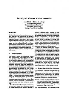
Ncalls 1 ∝ ¯ n k ¯ ∝ √n. and knowing that k Besides the planar square of unit area the figure also shows the results for nodes scattered on a unit–surface sphere and torus scenarios which are to represent different surface topologies. For the case of the sphere the capacity equals to that of the planar square – this was proven in [3] analytically. Actually the average path lengths in the n → ∞ limit do not differ for the two cases. This is not so for the case when all nodes at the border of the square are in the neighborship of the nodes at the opposite border of the square: the plane is folded into a torus. In this case the per node critical load ¯ is halved, the critical still decreases with √1n but because k load is twice than in the planar case, according to (2). Distance factor = 3
1
10
Sphere Torus Plane
3.1 Surface Topologies
We present an alternative approach to [3] for measuring the maximum traffic a stationary ad hoc network can deliver. Our heuristic model can be adapted for various surface topologies or changes in the traffic generation algorithm, and the model is able to provide the function relations between the parameters used. The idea for approximation of the capacity for given values of the network parameters is based on the averages of node utilization ui . The distribution of ui will be the same for a given blocking probability and normalized transmission range and thus we take the expectation value: u ¯. The total
0
Critical Load
In Figure 1 the per node critical load is plotted against the number of nodes for a normalized transmission range of 3. Our experience shows that for rN > 2.7 the graph is connected with high probability. We can see that the capacity decreases as √1n with the number of nodes. This can be attributed to the fact √ that the average path length of the calls increases with n thus one call uses up more and more capacity. An approximation of the overall throughput parameter can be given based on geometrical considerations as follows.
(2)
10
−1
10
−2
10
2
3
10
10
4
10
Number of nodes Figure 1: Distributing the nodes on a torus results in increased per node throughput for a given system size but the overall decay will not change.
3.2 Power Control In our next scenario we analyze the effect of an ideal power control implementation. In this case the hosts are able to
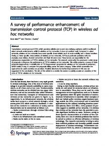
With the use of (2) we can predict the effect of the power control: the transmission ranges reduce, which causes the rhs to increase. Figure 2 shows the per node critical load parameter plotted against the size of the system. The results without power control are also given for comparison. It appears that the use of the power control mechanism can increase the capacity of the ad hoc network by as much as 35% for a given number of nodes but the system retains its overall worsening property with n → ∞.
Distance factor = 3 Plane Localization
Critical Load
change their transmission range according to the demand: they transmit with power just enough to reach the next node. The neighborship relations are still calculated using the normalized transmission range, which serves as maximum transmission range in this case, and actual transmissions affect only those nodes that are closer to the transmitting node then the next node in the path.
0
10
−1
10
2
1
Plane Torus Basic with Power Control Torus with Power Control
Critical Load
0
−1
10
−2 2
3
10
4
10
Number of nodes Figure 2: Using power control can result in +35% in the per node throughput, still the n−1/2 decrease remains as expected.
3.3 Localization of Traffic The decrease in throughput seems to persist for all investigated cases of n identical agents that are calling all other nodes with equal probabilities. It is possible, however, for different of communication behaviour to “break” the through¯ is constant, then put barrier. Note that (2) yields that if k 2 Ncalls = const also holds, because rN ∝ n. This way we ¯ = const. have only to find a way that makes k Let us change the traffic generation algorithm in a way to prefer short length calls. In this scenario calls are going to be generated with a certain probability depending on the number of hops along the shortest path connecting the source and destination nodes. Let h denote this path length in hops and let the probability function be the standard one: f (x) = e
4
10
Figure 3: The throughput of the localized network is not effected by the changes of the system size.
10
10
10
Number of nodes
10
10
3
10
Distance factor = 3
2 − h2 2σ
where σ plays the role of a cutoff parameter: the majority (' 67%) of the attempted calls are a maximum of σ hops long, thus the average path length values for different system sizes
will be similar. Figure 3 shows that in such simulations the per node critical load does not fall with increasing system sizes. Actually the per node throughput will constantly hold the same value as the one for the basic non-localized case of n0 nodes, where n0 depends solely on σ. We explain this behavior as follows. The traffic initiated by a single node will mostly affect those that are her 1st , 2nd , . . . , σ th neighbors. It means that a virtual subsystem of the size n0 is formed around each node: the traffic generated by a call now is limited to a much smaller environment. The traffic otherwise evolves in every such subsystem as in the whole system for the non-localized case, however, the limiting size now is n0 , not n. For σ = const n0 will not change with n, thus the throughput is constant for various system sizes. Figure 3 demonstrates a numerical example for comparison of the localized and non-localized cases. We have taken σ = 3, which yields that up to the 3rd neighbors of every node are in the subsystem. The expectation value for the count of the maximum 3rd neighbors of a node is in the range 40-60 – this agrees to the results of Figure 3, where at n0 ' 50 the per node throughput values for the two network traffic cases are nearly equal.
4. CONCLUSION In our paper we gave an alternative description of the maximum throughput for stationary ad hoc networks. Our model √ accounts for the O(1/ n) decay with increasing system sizes, and provides an intuitive way to acquire first order approximation concerning the effect of qualitative changes in the topology or traffic model parameters of the network. Examples were given to verify and support the heuristics, and in order to show the applicability of our model.
5. REFERENCES [1] S. Das, C. Perkins, and E. Royer. Performance comparison of two on-demand routing protocols for ad hoc networks. In Proc. IEEE Infocom, 2000.
[2] J. Gomez et al. A power-aware routing optimization scheme for mobile ad hoc networks. Work in Progress, draft-gomez-paro-manet-00, 2001.
[4] P. R. Kumar et al. Protocols for media access control and power control in wireless networks. Work in Progress, 2001.
[3] P. Gupta and P. R. Kumar. The capacity of wireless networks. IEEE Transactions on Information Theory, 46(2):388–404, 1999.
[5] J. Li, C. Blake, D. S. J. De Couto, H. I. Lee, and R. Morris. Capacity of ad hoc wireless networks. In Proc. ACM Mobicom, 2001.