Oct 8, 2007 - direct routes from each source to the corresponding destination; and (3) cell-based routes constructed by percolation rather than by simply ..... If a diamond contains at least one node, it is said to be open, and closed otherwise. .... any node located in any square within Manhattan distance d of the originating ...
Throughput Scaling in Random Wireless Networks: A Non-Hierarchical Multipath Routing Strategy
arXiv:0710.1626v1 [cs.IT] 8 Oct 2007
Awlok Josan, Mingyan Liu, David L. Neuhoff and S. Sandeep Pradhan Electrical Engineering and Computer Science Department University of Michigan, Ann Arbor, MI 48109
Abstract— Franceschetti et al. [1] have recently shown that per-node throughput in an extended (i.e., geographically expanding), ad hoc wireless network with Θ(n) randomly distributed nodes and multihop routing can be increased from the Ω( √n 1log n ) scaling demonstrated in the seminal paper of Gupta and Kumar [2] to Ω( √1n ). The goal of the present paper is to understand the dependence of this interesting result on the principal new features it introduced relative to Gupta-Kumar: (1) a capacity-based formula for link transmission bit-rates in terms of received signal-to-interference-and-noise ratio (SINR), instead of the threshold model that positive bit-rate W is attainable when SINR lies above some threshold, and zero bit-rate otherwise; (2) hierarchical routing from sources to destinations through a system of communal highways, instead of individual direct routes from each source to the corresponding destination; and (3) cell-based routes constructed by percolation rather than by simply interconnecting all cells touched by a straightline between two end points. The conclusion of the present paper is that the improved throughput scaling is principally due to the percolation-based routing, which enables shorter hops and, consequently, less interference. This is established by showing that throughput Ω( √1n ) can be attained by a system that does not employ highways, but instead uses percolation to establish, for each source-destination pair, a set of Θ(log n) routes within a narrow routing corridor running from source to destination. As a result, highways are not essential. In addition, it is shown that throughput Ω( √1n ) can be attained with the original threshold transmission bit-rate model, provided that node transmission powers are permitted to grow with n. Thus, the benefit of the capacity bit-rate model is simply to permit the power to remain bounded, even as the network expands.
I. I NTRODUCTION The problem of asymptotic scalability of throughput in wireless networks has been investigated extensively under different assumptions on the network models. The seminal work of Gupta and √ Kumar [2] demonstrated that per-node throughput Ω(1/ n ln n) was achievable as the number of nodes in the network, n, goes to infinity. Franceschetti et al [1] recently showed that this achievable per-node throughput may be increased. Specifically, they considered an extended (i.e., geographically expanding) network with approximately n randomly distributed nodes and multihop routing, and demonstrated that achievable per-node throughput can be increased to Ω( √1n ). Compared to [2], the construction used in [1] introduced several new features. The first is a capacity-based link This work was supported by NSF Grant CCF-0329715.
transmission rate formula as a function of the received signalto-interference noise ratio (SINR), instead of the thresholdbased binary rate model used in [2], where a positive bit-rate W is attainable when the SINR is above some threshold, and zero otherwise. (The former requires coding at each hop, while the latter does not.) The second is a routing hierarchy for data delivery in which data from a source is first delivered (via a single hop) onto a nearby highway – one of a system of communal highways, each with a horizontal and a vertical segment. The data is then multihopped along the highway (horizontally then vertically), and finally delivered from the highway to the destination in a single hop. By contrast, the method used in [2] is a simple shortest path type of routing, where a straight line is drawn connecting the source and the destination, and nodes along this line are selected to relay the data, forming an approximately straight line path. The third difference introduced in [1] is the use of percolation theory to construct the highways that serve as the main routing fabric in the network. Indeed, [1] is the first paper to use percolation theory to establish network throughput results. The primary interest of the present paper is to understand which of the above contribute to the increase in per-node throughput in a fundamental way, i.e., to understand the dependence of this new result on the above new features. The conclusion of this paper is that the improved throughput scaling is principally due to the percolation-based routing, which enables shorter hops and, consequently, less interference. More precisely, the hops along the highways have bounded lengths that do not increase as the network expands. This would not have been possible if one were to use shortest path routing, the existence of which then invokes a connectivity requirement that would force the hop size to increase as the network expands. This conclusion is established by showing that throughput Ω( √1n ) can be attained by a system that does not employ highways, but rather uses percolation to establish, for each source-destination (s-d) pair, a set of Θ(log n) disjoint routes within a narrow routing corridor running from source to destination. Thus with this multipath routing structure, highways and routing hierarchy are not essential. In addition, it is shown that throughput Ω( √1n ) can be attained with the original threshold transmission bit-rate model, provided the transmission powers of the nodes are permitted to grow with n. Thus, the benefit of the capacity bit-rate model is simply to permit the power to remain bounded, even as the network
expands. The remainder of the paper is organized as follows, Section II introduces the system and the transmission rate models we use. Section III gives our main result and an overview of the proof. The formal proof follows in sections IV, V, VI and VII, which formalize the path construction, data rates, loading factor and the system scheduling, respectively. II. S YSTEM M ODEL We consider the random extended network, which consists 2 of √ a set of nodes distributed over a disk An ⊂ R with radius n, called the network region. We construct the network by placing the nodes according to a Poisson point process of unit intensity over R2 and focusing our attention to the network region An . We denote the location of the ith node by si . Each node, si , serves as a source of bits which it wishes to communicate to a destination, denoted by di , which is chosen randomly from the remaining nodes. Each node may serve as a destination for more than one source. Communication is done using a multihop relaying scheme under a slotted time system. There is a transmitter and receiver at each node. All transmitters use the same power P , which we get to choose and which may depend upon n. We assume that node j receives the transmitted signal from node i with power P η(dij ), where η is a propagation model and dij is the Euclidean distance between nodes i and j. We use the propagation model introduced by Arpacioglu and Haas [3], 1 , η(d) = (1 + d)α
(1)
where α > 2 is a constant depending upon the channel conditions. A. Transmission Rate Models Let t be a set of simultaneously transmitting nodes. Then the SINRij (signal to interference and noise ratio) at node j when node i is transmitting to it is given by SINRij =
N0 +
P η(d ) P ij . k∈t P η(dkj ) k6=i
We use two different transmission rate models. Model A In this model, which was used in [1], the transmission rate is equal to the capacity of the wireless channel. That is the rate (in bits/sec) at which node i can transmit to node j is 1 W T ln(1 + SINRij ) , (2) 2 where W is the bandwidth and T is length of the time slot. Model B In this model, which has been more commonly used in throughput analysis of wireless networks [2]–[4] the transmission rate is � B if SINRij ≥ τ Rij = , (3) 0 else Rij =
where τ is some pre-determined threshold and B is a number less than channel capacity.
III. M AIN R ESULT In the following theorem, which is √ our main result, we demonstrate the achievability of Ω(1/ n) throughput for both transmission rate models, using a non-hierarchical routing strategy, i.e., without the use of highways. Theorem 1: Under transmission Models A and B, a per√ node throughput of Ω(1/ n) bits/sec is achievable in the random extended network. Under Model A the throughput is achievable with any constant finite power P at each node, whereas under Model B the throughput is achievable only if power P increases to infinity as n → ∞. We now give an overview of the proof, details of which are in subsequent sections. For each s-d pair we find with high probability Ω(ln n) disjoint routes (i.e., a sequence of hops from node to node) from source to destination such that 1. each route consists of a draining hop from the source, a path consisting of a sequence of intermediate hops, and a delivery hop ending at the destination, 2. the first hop, i.e., the draining hop, has length O(ln n) and extends from the source to the first node of the path, 3. the last hop, i.e. the delivery hop, has length O(ln n), and extends from the last node of the path to the destination. 4. all intermediate hops have lengths bounded by a constant not depending on n. To make the analysis tractable, we modify these paths slightly in a way that preserves their distance properties, but does not necessarily preserve their disjointness. √ We then show that for each s-d pair, a rate of Ω(1/( n ln n)) is sustainable on each hop of each of its modified paths. To do this, we show that the maximum number of sourcedestination paths on which an intermediate node can lie is √ O( n ln n). From Item 4 above, the intermediate nodes, with the exception of the delivery node, transmit over a bounded distance. Theorem 3 of [1] showed that when transmitting over a bounded distance, nodes can maintain a throughput of Ω(1). Thus for each s-d pair an√intermediate node√can sustain a throughput of Ω(1) × 1/O( n ln n) = Ω(1/( n ln n)). Next, using Theorem 3 of [1] again, we show that a source √ can transmit data at rate Ω(1/ n) in a way that will be received by a node on each of the Ω(ln n) paths for the s-d pair. Through this node, each path then takes a share of this √ rate equal to Ω(1/( n ln n)). Therefore, the source√is able to drain onto each of the Ω(ln n) paths at rate Ω(1/( n ln n)). Similarly, delivery√nodes can deliver data to the destination at a rate of Ω(1/( n ln n)) from each path. Combining the above results we see that, for each sourcedestination pair we have √ Ω(ln n) routes, each of which can sustain a rate of Ω(1/( n ln n)). √ Thus the per-node√throughput is given by Ω(ln n) × Ω(1/( n ln n)) = Ω(1/ n). IV. PATH C ONSTRUCTION
VIA
P ERCOLATION
In this section we show that, with probability approaching 1 as n → ∞, there exist Ω(ln n) suitable disjoint paths for each source-destination pair. Here the probability is with
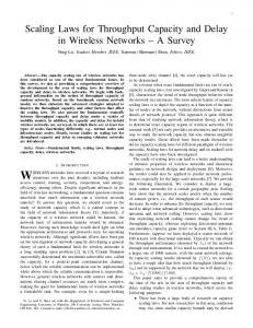
If a diamond contains at least one node, it is said to be open, and closed otherwise. Draw horizontal edges across half the diamonds and vertical edges across the others in the manner shown in Figure 1(b). An edge is considered open if it lies in an open diamond, and closed otherwise. Define a path as a sequence of connected edges, horizontal or vertical. A path is said to be open if it contains only open edges. We will show that there are Ω(ln n) disjoint open paths crossing the routing corridor lengthwise, i.e. beginning at the left and ending at the right side of the routing corridor. Let Im be the event that there exist at least m disjoint open paths that cross the routing corridor lengthwise. The following lemma, whose proof can be found in the proof of Theorem 5 of [1] is based on an important result from percolation theory.
c
√
2cκ ln
√ √n 2c
√ 2 n (a) Tessellation of a rectangular routing corridor with diamonds of side length c. √
2c
√
√
n 2cκ ln √2c
√ 2 n (b) Paths crossing the routing corridor from left to right are composed from horizontal and vertical edges, shown as dashed lines. Fig. 1.
Routing corridor setup for finding paths for a given s-d pair.
respect to the Poisson point process for node locations and the random destination assigned to each source node. To do this, we use the percolation approach that was used in [1] to establish the existence of suitable highways. Here we apply approach to find a set of suitable paths for each sourcedestination pair. Since we need to show the existence of paths for every s-d pair, we first need to upper bound the number of nodes in the network region An , which we denote Nn . Lemma 1: The probability that the number of nodes, Nn , in the network region An is less than 2πn goes to 1 as n goes to infinity. Proof: The number of nodes in the network region, Nn , is a Poisson random variable with mean πn. Applying the Chernoff bound gives, Pr(Nn > 2πn) ≤ e−2sπn E[esNn ] = e−2sπn eπn(e
s
−1)
=1−e
We now set up a routing corridor for each s-d pair. The following theorem demonstrates that when n is large, with high probability there are Ω(ln n) disjoint paths in each one of those corridors. Theorem 2: Given κ > 0 and c > ln 6 + 4/κ, there exists a strictly positive constant β(c, κ) such that if for every n we are √ given at √ most ⌈2πn⌉ routing corridors of dimensions √ n in R2 , then with probability approaching 2 n× 2cκ ln √2c √
n one there exist m = βκ ln √2c disjoint open lengthwise crossing paths within each of the routing corridors.
Observe that when n are large, the routing corridors are quite narrow. Proof: We prove this theorem using Lemma 2 and the union bound. It suffices to assume that we have ⌈2πn⌉ routing corridors. Then Pr(all ⌈2πn⌉ routing corridors have m disjoint open paths)
for all s > 0. Choosing s = 1 gives Pr(Nn ≤ 2πn) ≥ 1 − e
Lemma 2: Given arbitrary constants κ, c > 0, there exists a strictly positive constant β = β(c, κ) such that 4 � n �a (4) Pr(Im ) ≥ 1 − 3 2c2 √ � n where m = βκ ln √2c and a = 21 (β − 1)κc2 + κ ln 6 + 1 .
= 1 − Pr(at least one routing corridor has less that m disjoint open paths)
−2πn πn(e−1)
e
πn(3−e)
�
→ 1 as n → ∞ .
Next we prove that for a given s-d pair, there are Ω(ln n) disjoint paths such that the distance to (from) each path from (to) the source (destination) is O(ln n), and that every intermediate hop along each path is of length O(1), i.e. its length is upper bounded by a constant independent of n. To show this, we consider a√ rectangular routing corridor of √ √ n in R2 that includes both s dimensions 2 n × 2cκ ln √2c and d, where c, κ > 0 are constants to be chosen later. Tessellate this routing corridor with diamonds of side c as shown in Figure 1(a). Then for any given diamond, 2
Pr(diamond contains at least one node) = 1 − e−c , p .
≥ 1−
⌈2πn⌉
X
Pr(ith routing corridor has
i=1
less than m disjoint open paths) ≥ 1 − ⌈2πn⌉ · Pr(a routing corridor pair has
less than m disjoint open paths) = 1 − ⌈2πn⌉(1 − Pr(Im )) 4 � n �a ≥ 1 − 8n · 3 2c2 32 = 1− na+1 3(2c2 )a where the first inequality follows from the union-bound and the second inequality uses Lemma 2. Note that the above
s
√ 2 n d
√
n
√ √ n 2c ln √2c
we replace it with the designated relay node. In this way we obtain a set of Ω(ln n) paths for each s-d pair such that each source (destination) is within O(ln n) of each of its paths. Note, however, that now the √ maximum √ intermediate hop length has been increased to ( 5 + 2)c. Moreover, the paths corresponding to one s-d pair might no longer be disjoint. For example, in two originally disjoint paths there might be a node in one path and a node in the other that are contained in adjacent diamonds in the original tesselation of the routing corridor, but are in the same square of the new tesselation of the entire network region. In this case, the two modified paths share a common relay node. V. DATA R ATES
Fig. 2. For a given s-d pair the orientation of the routing corridor on the network region.
expression goes to one as n tends to infinity if a < −1. Given κ > 0 and c > ln 6 + 4/κ, choosing β(c, κ) = 1 − (κ ln 6 + 4)/(κc2 ) > 0 results in a < −1. �
Corollary 1: Given κ > 0 and c > ln 6 + 4/κ, there exists a strictly positive constant β(c, κ) > 0 such that with probability approaching one there exist Ω(ln n) disjoint open paths for each s-d pair such that the distance path √ from √ of any √ the source and destination is less than 2cκ ln(√ n/ 2c) and every intermediate hop has length less than 5c.
Proof: For any given s-d pair, consider a routing corridor with the aforementioned dimensions such that it contains both source and destination and that the portion of the routing corridor that intersects the network region is as high as possible (see Figure 2). According to Lemma 2, with high probability there are Ω(ln n) disjoint open paths that cross the routing corridor lengthwise. Now consider the part of the routing corridor that lies within the network region. Since there are Ω(ln n) disjoint open paths that cross the routing corridor lengthwise, there will be Ω(ln n) disjoint open paths in the truncated region √ Also, since the width of the √ as well. n , the minimum distances of routing corridor is 2cκ ln √2c each of these paths from the source and the destination is √ √ n less than 2cκ ln √2c . Also, using a geometric argument, it √ is easy to see that any intermediate hop has less 5c or less. Theorem 2 shows the existence of paths for a number of routing corridors no larger than ⌈2πn⌉. Using the above construction for every s-d pair and combining with the fact that the number of s-d pairs is less the 2πn with high probability (Lemma 1) completes the proof of the corollary. � As suggested earlier, for tractability we need to modify the paths provided by the corollary. Ignoring the previous tesselations of routing corridors, consider now a tessellation of the entire network region into squares of side c. If a square has multiple nodes in it, we designate one node as the relay node. Now, for every hop of every s-d path, if the node that is to transmit is not the designated relay node for the square,
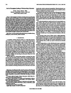
We begin this section by finding a lower bound on the per-node transfer rate when for some D > 0 every node has to send data to all nodes within distance D of itself. This involves setting up a TDMA schedule so as to limit the number of simultaneous transmissions taking place, which in turn limits the interference. Corollaries are then given for use in the proof of the Theorem 1. For transmission rate Model A, Theorem 3 of [1] can be used. The following extends this theorem to transmission rate Model B. Theorem 3: Given c > 0, given a tessellation of the network into squares with sides of length c, and given an integer d > 0 there exists a rate R(d) = Ω(d−α−2 ) using Model A and R(d) = Ω(d−2 ) using Model B such that one node in each square can successfully transfer data at rate R(d) to any node located in any square within Manhattan distance d of the originating square (i.e. d or fewer horizontal and/or vertical steps). The asymptotic behavior of the rate under Model A can be attained by any fixed finite power at each node. However to achieve the rate under Model B we have to let power P go to infinity as d tends to infinity. Proof: For Model A the proof is given in [1, Theorem 3], and for the extension to Model B, we now make a similar construction. We consider a partition of the network region into super-squares, each composed of k 2 smaller squares, for some k to be chosen later. We index the squares in each super-square starting in the lower left corner, moving horizontally in the bottom row from left to right, and then in the row above it from left to right, and so on. We set up a TDMA schedule of k 2 slots such that in the ith slot, from every square indexed by i, precisely one node can transmit. Consider a transmitter-receiver pair separated by d squares. Choosing k = x(d + 1), where x = max(2, ⌈(16τ γ)1/α (1 + 1/(2c))⌉) , P∞ and γ = i=1 (i − 1/2)−α+1 , we can see that the closest 8 interferers are at least x(d + 1) − d squares away, the next closest 16 interferers are at least 2x(d + 1) − d squares away, and so on (Figure 3). The power from interfering nodes can
� + 1+
k=2(d+1)
d
Fig. 3. Construction for lower bound on SINR. The shaded square at the center is the actual signal, all other shaded squares are interfering transmitters. In the above figure d = 1.
thus be upper bounded as PI (d) ≤ =
∞ X
i=1 ∞ X i=1
≤ 8P = ≤
8iP η(c(ix(d + 1) − d)) 8iP (1 + c(ix(d + 1) − d))α
∞ X i=1
i (c(d + 1)(ix − 1))α
∞ X i 8P α α α c (d + 1) x i=1 (i − 1/x)−α ∞ X 8P 2(i − 1/2) α α α c (d + 1) x i=1 (i − 1/2)−α
∞ X 16P (i − 1/2)−α+1 = α c (d + 1)α xα i=1
=
16P γ . cα (d + 1)α xα
Next we lower bound the signal power at the receiver. The Euclidean distance between the transmitter and receiver is at most c(d + 1). Thus the signal power, PS (d), satisfies PS (d) ≥ P η(c(d + 1)) P . = (1 + c(d + 1))α Using the above two bounds we obtain a bound on the SINR: PS (d) N0 + PI (d) P (1 + c(d + 1))−α ≥ N0 + 16P γ(2c)−α x−α �α �� 1 N0 = 1+ c(d + 1) P
SINR(d) =
1 c(d + 1)
�α
16γ xα
�−1
.
It can be easily shown that the second term in the above equation is less than 1/τ . Choosing P large enough that the sum of two terms still remains less than 1/τ results in SINR> τ . In this case according to Model B, one node in each square can transmit at rate 1 in such a way that all nodes within Manhattan distance d will successfully receive the transmissions. Since each square is allowed to have a transmitting node once every k 2 = x2 (d + 1)2 time slots, to get the asymptotic behavior we need to divide the above transfer rate by d2 . Thus under Model B, R(d) = Ω(d−2 ) is attainable. � We now give a corollary to the above theorem that will be used to show an achievable data delivery rate to the destination. Corollary 2: Given c > 0, given a tessellation of the network into squares with sides of length c, and given an integer d > 0 there exists a rate R(d) = Ω(d−α−2 ) for Model A and R(d) = Ω(d−2 ) for Model B such that one node in each square can receive data at rate R(d) from a transmitter located in any square within Manhattan distance d of the receiving square (i.e. d or fewer horizontal and/or vertical steps). Proof The proof is obtained by switching the role of transmitters and receivers in the proof of the previous theorem. � We conclude this section with three corollaries that use Theorem 3 to establish rates at which, respectively, draining, delivery and transmission along the intermediate hops can proceed. Corollary 3: With probability approaching one, every source node in the network can transmit to every one of the Ω(ln n) paths in its corresponding routing corridor at a rate Ω((ln n)−α−4 ) under transmission Model A, and Ω((ln n)−4 ) under Model B. Proof: First, for Model A, consider the tessellation of An into squares of side length c. Consider also any one source node. Since the Manhattan distance from this source to each of its paths is less than φ ln n, for some φ > 0, if this node is the only node within its square then Theorem 3 with d = φ ln n implies it can transmit data that is successfully received by a node on each of its paths at rate R(φ ln n) = Ω((ln n)−α−2 ) . It is therefore decided that nodes will transmit at rate Θ((ln n)−α−3 ), and since each path takes responsibility for relaying an equal share of this data, each path is responsible to relay Θ((ln n)−α−4 ). When n is large, with high probability the number of nodes in a square of size c is O(ln n) [1, Lemma 1]. Every node can actually transmit data at rate of Θ((ln n)−α−4 ). The proof for Model B follows similar arguments. �
Corollary 4: With probability approaching one, every destination node in the network can receive data from every one of the Ω(ln n) paths in its corresponding routing corridor at a rate Ω(ln n)−α−5 ) under Model A, and Ω((ln n)−5 ) under Model B. Proof: First, for Model A, consider a tessellation of An into squares of side length c. Consider any one destination node and one of the source nodes that corresponds to that destination. Since the distance to the destination from each of its paths is less than φ ln n, for some φ > 0, if this node is the only node within its square then Corollary 3 implies that data can be successfully received by the destination at rate R(φ ln n) = Ω((ln n)−α−2 ). It is therefore decided that nodes delivering data to this destination will transmit at rate Θ((ln n)−α−2 ). Using the Chernoff bound we can easily see that the number of sources that choose any given node as its destination is O(ln n) with high probability. Setting up a TDMA scheme in which each epoch consisting of O((ln n)2 ) slots would allow the destination to receive from every path of every source that selects the given node as its destination at least once in every epoch. Thus a destination can receive at rate Ω((ln n)α−4 ). When n is large with high probability the number of nodes in a square of size c is O(ln n) [1, Lemma 1]. Thus every node can receive data at rate Ω((ln n)−α−5 ). The proof for Model B follows similar arguments. � Corollary 5: Given c > 0, and a tessellation of An into squares of side length c, one node in every square can transmit to every node located within distance O(1), i.e., distance is upper bounded by a constant that does not depend upon n, at a constant rate that does not depend upon n. Proof: First consider Model A. From Theorem 3 we know that one node in every square can achieve a rate of Ω(d−α−2 ) while transmitting to every node located within Manhattan distance d of the originating square. For transmissions over distance that is upper bounded by a constant not depending upon n, d would be a constant. Hence rate Ω(1) is achievable over constant distance. The proof for Model B follows similar arguments. � VI. L OADING FACTOR The loading factor of a designated relay node is the number of s-d paths on which it lies. We also consider it to be the loading factor of the square containing the relay node. In this section we find a probabilistic upper bound to the maximum loading factor among all squares, which then upper bounds the maximum loading factor of all relay nodes. Let Li (n) represent the loading factor of the ith square, and let L(n) = maxi Li (n). We observe that if an s-d pair contributes a path or paths to the Li (n), then it must be that the corresponding routing corridor intersects the ith square. Now, we observe that if the ith square intersects a given s-d routing corridor, it can, at most, intersect 9 diamonds of the routing corridor tessellation. Recall that the tentative paths for a given s-d pair are disjoint, i.e. a diamond of the s-d routing corridor can lie on only one tentative path. Thus, if
√ √c 2
s
r
√
√ (c/ 2) (r √ r 2 −(c/ 2)2
+
√
n)
n
Fig. 4. The ith square lies on a s-d path only if the destination lies in the striped region.
the ith square intersects the s-d routing corridor it may have to service at most 9 paths corresponding to that s-d pair. Therefore as an upper bound to L(n), we upper bound the number of s-d routing corridors that intersect any given square and multiply that number by 9. Theorem 4: For a tessellation of the network region into squares of side c, there exists a constant δ such that √ Pr(L(n) ≤ δ n ln n) → 1 as n → ∞ . Proof: √ √ Pr(L(n) ≤ δ n ln n) = Pr(max Li (n) ≤ δ n ln n) ≥1−
i M n X
√ Pr(Li (n) > δ n ln n)
i=1
(5)
πn c2
where Mn ≈ is the number of squares in the network PNn region. We have Li ≤ 9 j=1 Aij where Aij = 1 if the ith square intersects the routing corridor corresponding to the jth s-d pair and Aij = 0 otherwise. Note that for a given i, Ai1 , Ai2 ... are independent and identically distributed. However the Li ’s are not identically distributed. Instead Li will generally have a higher value for squares near the center of An than its boundary. The following lemma, which gives a uniform upper bound to pn,i , Pr(Aij = 1),√will be used to find a lower bound to the term Pr(Li > δ n ln n) that appears in (5). √ Lemma 3: Given c > 1/ 2 there exists µ such that √ (6) pn,i ≤ pn , µ ln n/ n , for all n, i . Proof: We setup a polar coordinate system such that the origin lies at the center of the network region. As the probability of intersection of a square by a random s-d pair routing corridor is highest at the center, we consider the ith square to lie at the center of the network region, i.e., to contain the origin. Since such a square of side c is completely √ contained in a circle of radius c/ 2, we upper bound pn,i by the probability of a random s-d routing corridor intersecting √ a circle of radius c/ 2 centered at the origin.
For a source located at (r, θ), the probability that square i is intersected by the s-d pair routing corridor is upper bounded by the probability of the destination lying in the striped regions √ of Figure 4. Since the diameter of the network region is 2 n, the area of the horizontally √ striped regions can √ √ √ n be upper bounded by 2 · 2 n · 2cκ ln √2c . Since c > 1/ 2 √ √ the upper bound can be relaxed to 2 n · 2cκ√ln n. Also, the area of the vertically striped portion is √ 2(c/ 2)√ 2 (r + r −(c/ 2) √ 2 n) . Therefore
� � 3 = 1 − exp −27πnpn ln + ln Mn e � µ ln n 3 = 1 − exp −27πn √ ln + e n πn � ln 2 c → 1 − 0 = 1 as n → ∞ , which concludes the proof of Theorem 4. VII. S YSTEM S CHEDULING
�
Pr (s-d routing corridor intersects square i|s = (r, θ)) ( 1 if r ≤ c √ √ √ ≤ (r+ n)2 (c/ 2) n 2 2κc ln √ + √ otherwise
In this section we explain a system protocol that achieves √ a per-node throughput of Ω(1/ n) and complete the proof of Theorem 1. √ π πn n r 2 −(c/ 2)2 For every path corresponding to an s-d pair we designate Since the joint probability density of the polar coordinate the node on the path that is closest to the source (destination) 1 locations is p(r, θ) = 2r as the draining (delivery) node. We cycle among three n 2π , we have √ Z 2πZ n � � different categories of time slots: draining, relaying and s-d routing corridor Pr pn,i = s = (r, θ) p(r, θ) drdθ delivery. In draining slots, the source transmits its packets intersects square i 0 0 to the designated draining nodes. In the relaying slots, the √ Z √n Z c 2 2κc ln n 2r relaying nodes transmit the data towards the destination. √ + dr + ≤ π n Finally in the delivery slots, the delivery nodes transmits c 0 n the data to the destination. √ √ 2 (c/ 2) (r + n) 2r Theorem 4 shows that the maximum number q dr √ of s-d paths √ πn n n ln n). Since that a relaying node may have to serve is O( 2 2 r − (c/ 2) all relaying nodes can transmit at rate Ω(1) (Corollary 5), √ √ √ ln n c2 2 2κc ln n the relaying node can maintain a throughput of Ω(1/ n ln n) √ + (c/ 2) √ ≤ + n π n n per path. ! √ From c c ln n 1 2 2κ √ Corollaries 3 and 4, it is easy to see that a rate of √ = √ +√ + Ω(1/( n ln n)) per path can be maintained in the draining π n ln n n 2 and the delivery phase. ln n Thus every s-d pair can achieve a rate of ≤ µ √ , pn n � � � � √ 1 1 where µ = c(2 + (2 2κ)/π). � √ bits/sec/path × Ω(ln n) paths = Ω √ bits/sec Ω n ln n n Returning to the proof of Theorem 4, since Li ≤ (7) P Nn Aij , we have 9 j=1 which completes the proof of Theorem 1. Nn X Aij ] = 9 E[Nn ] E[Aij ] = 9πnpn,i ≤ 9πnpn . E[Li ] ≤ 9 E[ j=1
Applying the Chernoff bound [4, Lemma C3], � � 3 Pr(Li > 27πnpn ) ≤ exp −27πnpn ln . e Substituting the above into (5) and choosing δ = 27π gives � � Mn X √ 3 exp −27πnpn ln Pr(L(n) ≤ δ n ln n) ≥ 1 − e i=1
R EFERENCES
[1] M. Franceschetti, O. Dousse, D. Tse and P. Thiran, “On the throughtput capacity of random wireless networks,” to appear in IEEE Trans. on Inform. Theory. [2] P. Gupta and P. R. Kumar, “The capacity of wireless networks,” IEEE Trans. Inform. Theory, vol. 46, pp. 388-404, Mar. 2000. [3] O. Arpacioglu and Z. Haas “On the scalability and capacity of wireless networks with omnidirectional antennas,” IPSN, Berkeley, Apr. 2004. [4] E. Duarte-Melo, A. Josan, M. Liu, D. L. Neuhoff and S. Pradhan, ”The effect of node density and propagation model on throughput scaling of wireless networks,” submitted to IEEE Trans. on Inform. Theory