INTRODUCTION. The transport capacity (TC) of a wireless network has been a topic of great interest since the paper [4]. The TC of a wireless network indicates ...
Throughput Versus Routing Overhead in Large Ad Hoc Networks (Invited Paper) Radha Krishna Ganti and Martin Haenggi Department of Electrical Engineering University of Notre Dame Notre Dame, IN 46556, USA {rganti,mhaenggi}@nd.edu ABSTRACT Consider a wireless ad hoc network with n nodes distributed uniformly on [0, 1]2 . The transport capacity (TC) of such a √ n. To achieve this, each node wireless network scales like √ should serve about n distinct information flows.√So the routing table of each node should be of the order n bits. We show that if the size of the routing table is restricted to be of the order O(nH(δ) ), the maximum achievable pernode TC is O(nR(δ) ) when the source-destination ˘ ¯ distance is n−δ/2 . We show that R(δ) = min 12 , 2δ + H(δ) − 1 is the optimal tradeoff.
x8 x7
x6 x9
Keywords Wireless networks, ad hoc networks, routing overhead, transport capacity.
1.
x3 x1
x4
x5
x2
INTRODUCTION
The transport capacity (TC) of a wireless network has been a topic of great interest since the paper [4]. The TC of a wireless network indicates how far and how fast information can be propagated in a network. When all the source-destination distances are of the same order, the TC is proportional to the sum rate that can be achieved by the network. It was shown in [4] that the TC of n “ wireless nodes ” p uniformly distributed in a unit square is Θ n/ log(n) when all the nodes have a common transmission range. Here each source has a destination at Θ(1) distance away. Later the log(n) factor in the denominator was removed in [2] by using variable transmission ranges. In both the above results, interference is treated as noise. A lot of work has been done in understanding the TC of a wireless network with fading and when interference is not treated as noise [5]. In the ad hoc networks, routing is intricately related to scheduling, the hop lengths and hence the TC of the network. Also there is a cost associated for establishing the
Permission to make digital or hard copies of all or part of this work for personal or classroom use is granted without fee provided that copies are not made or distributed for profit or commercial advantage and that copies bear this notice and the full citation on the first page. To copy otherwise, to republish, to post on servers or to redistribute to lists, requires prior specific permission and/or a fee. WICON’08, November 17-19, 2008, Maui, Hawaii, USA. Copyright 2008 ACM 978-963-9799-36-3 ...$5.00.
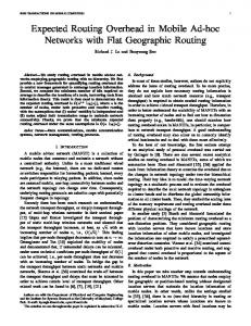
x10 Figure 1: Illustration of a routing table
routes a priori or dynamically. The routing table has to be stored in the wireless device. If the number of nodes in the network scales, it is not very clear how the size of the routing table should scale and how this would affect the TC of the network. In [7, 1, 6] the routing overhead is considered in a mobile ad hoc networks. They formulate the problem of overhead in a mobile ad hoc network as a rate distortion problem and provide the overhead as function of the mobility parameters. In this paper we focus on the routing table length that each node has to maintain. To illustrate the overhead we are indicating, consider a wireless network in which the nodes are arranged on a lattice grid. See Figure 1. A basic overhead in a network would be to indicate the source and destination address in a packet. For a network of n nodes this would scale like O(log(n)) bits per packet, and this overhead cannot be avoided. So each packet has a source number and a destination number that is included in it. The scheduling is done such that all the eight neighbors of a node remain silent when it is transmitting. We also assume that the routing tables are set before the network begins to operate. Suppose x2 wants to transfer a packet stream to x8 . One possible route is indicated in a dashed
line. The packet moves in hops as x2 → x3 → x4 → x5 → x6 → x7 → x8 . Each node xi , 2 < i < 8 has an entry in the routing table that tells the node what to do if it receives a packet with source x2 and destination x8 . In this strategy all the nodes in the path of the flow should have routing information about that flow. So in the above example six nodes have routing information about the flow (x2 ⇒ x8 ). We quantify the trade-off in the scaling between the transport capacity and the size of the routing table as a function of the distance that a packet propagates.
2.
SYSTEM MODEL
Consider an ad hoc network with n nodes that are uniformly distributed on the unit square S = [0, 1]2 . We assume that a node located at x can communicate to a node located at y if SINR(x, y) > ν i.e., we are considering interference as noise. We make the following assumptions: 1. ν > 1. 2. The path loss model is given by kxk−α , α > 2. 3. Nodes are unaware of their locations, i.e., do not have a GPS receiver built into them. Each node is identified by its node ID. 4. Each node is randomly paired with a destination at a distance Θ(n−δ/2 ), δ ∈ [0, 1], i.e., each packet has to traverse a distance of Θ(n−δ/2 ). 5. Time is slotted. 6. All source nodes should support the same per-flow throughput λ. We also assume that a node is able to transmitt one packet in each time slot if SINR > ν. So if each source node is able to deliver K packets generated by it to its destination in T time slots, then limT →∞ K(T )/T = λ. Also if the modulation type and the packet size are fixed for all the nodes and hops, the packet rate λ would be proportional to the per-node bit rate.
destination when the packet size scales with the permitted per-flow throughput. Later they extended the result to the case of fixed packet length. So we define the delay exponent as D(δ) = lim
n→∞
3.
log(Average # hops required by the flows) log(n)
UPPER BOUND ON THE TRANSPORT CAPACITY
We now bound the TC of n nodes with the average number of hops that a packet takes to reach its destination. We closely follow the proof of Theorem 2.1 in [4]. Theorem 1. Consider an ad hoc network with n nodes which satisfies the conditions given in the previous section. Then ff 1 δ , + D(δ) (1) R(δ) ≤ min 2 2 Proof. This is very similar to the upperbound proved in [3] except that we state the dependence on δ ∈ [0, 1] explicitly. Let the k-th packet1 take hk (n) hops to reach its destination. Let λ denote the per node throughput of each node. Denote the hop set that a packet flow i takes to reach its destination by o n h (n) . Ei = x1i , x2i , . . . , xi i We use xki to denote both the hop and its length. Let Γm denote the set of active hops (transmitters and receiver pairs) at time instant m. Since each node ( its packet flow ) supports a rate of λ we have min i∈{1,...,hi (n)}
n→∞
log(per-flow transport capacity) log(n)
and the routing table size overhead exponent to be log(per-node routing table size) H(δ) = lim n→∞ log(n) We characterize R(δ) as a function of H(δ). Observe that we can restrict the per-node routing table size independent of δ. For example we can choose the routing table size to be nβ/2 , β ∈ [0, 1]. Then H(δ) = β/2. It was shown in [3] that the average delay is equal to the average number of hops that a packet takes to reach its
(2)
for large T . This is basically the average rate constraint. We also have the following constraint on the transmitting set at every time instant. X 2 x ≤ A, (3) x∈Γm
where A is some constant. This follows from the sphere packing bound. From (3), we have
With the above assumptions the per-node transport capacity is given by λn−δ/2 and the TC is given by λn1−δ/2 . Observe that the TC is proportional to the per-flow (per-source node) throughput λ. We define the rate exponent to be R(δ) = lim
T 1 X 1Γ (xik ) = λ, 1 ≤ k ≤ n T m=1 m
T X X
x2 ≤ T A.
(4)
m=1 x∈Γm
Since each packet has to travel over a distance n−δ/2 , we have hk (n)
X
xik ≥ n−δ/2 , 1 ≤ k ≤ n.
(5)
i=1
Rewriting (4), we have T X n hX k (n) “ ”2 “ ” X xik 1Γm xik
≤ TA
m=1 k=1 i=1 1 We identify the packets by the node number from which they originate.
Interchanging the summations and using (2), we have n hX k (n) “ X
xik
”2
≤ Aλ−1
(6)
k=1 i=1
From the Cauchy-Schwartz inequality we have v uhk (n) hk (n) uX X i 2 xk ≤ t (xik ) hk (n). i=1
p ho
Using (5), we have X
xik
−δ
”2
≥
i=1
n . hk (n)
(7)
λ
k=1
n−δ ≤A hk (n)
δ/2+1
≤ An
λn
n X k=1
Observe that n
“P
n 1 k=1 hk (n)
”−1
1 hk (n)
Long S-D
D(δ)
So we have 1−δ/2
δ
Short S-D
Figure 2: The rate-exponent region as a function of δ
Using (7) in (6), we have2 n X
Extreme multihop
1111111111111 0000000000000 1010 0000000000000 1111111111111 0000000000000 1111111111111 1010 0000000000000 1111111111111 0000000000000 1111111111111 1010 0000000000000 1111111111111 0000000000000 1111111111111 10 101111111111111 0000000000000 1010 1 10100 10
0.5
gle Sin
i=1
hk (n) “
Everyone talks to NN
R(δ)
111111111111 000000000000 000000000000 111111111111 1010 000000000000 111111111111 000000000000 111111111111 1010 000000000000 111111111111 000000000000 111111111111 1010 000000000000 111111111111 000000000000 111111111111 10 0111111111111 0 1 000000000000 10 1 1010 10 10
0.5
!−1
M os th op s
is the harmonic mean of
hk (n). Using the fact that harmonic mean is smaller than arithmetic mean we have ! n 1X λn1−δ/2 ≤ Anδ/2 hk (n) (8) n k=1 √ From [4], we have TC(n) ≤ O( n). Taking the logarithm of (8), dividing by log(n) we have ”9 “ Pn 8 k=1 hk (n) = < log n log(TC(n)) log(c) 1 δ + ≤ min , + . ; log(n) :2 2 log(n) log(n) (9) Taking the limit of (9) we have the result.
δ
Single-hop
Short S-D
Long S-D
Figure 3: The delay-exponent region as a function of δ number of hops required to reach its destination, we then have from the previous theorem Average packet overhead n1−δ In the next theorem we provide a bound on R(δ) for a given H(δ). λ≤A
In Figure 2 we plot the feasible region of the rate exponent R(δ) as a function of δ. In Figure 3, we plot the corresponding region for the delay exponent. These two regions are related by the above theorem. Suppose all the packets reach the destination in an equal number of hops,
Theorem 2. We have R(δ) + 1 ≤ min
hi (n) = nγ , γ < 1. We then see that it is not beneficial to have γ greater than (1 − δ)/2. If we use nearest neighbor routing, the average number of hops requires for a packet to route a distance n−δ/2 is n(1−δ)/2 . So we have √ δ/2 + (1 − δ)/2 = 1/2 which implies that the TC scales like n for nearest neighbor routing. In a packetized network, each hop incurs some cost. The cost may be for initiating the hop or to maintain the link until the packet is transmitted. So if we assume that the overhead associated with each packet is proportional to the
1 δ , + H(δ) 2 2
ff
Proof. Let each node have information about kn other nodes. Denote the set of nodes which have information about node i by Ai . We then have n X
|Ai | = nkn
i=1
Since only |Ai | nodes know how to route the packet i, the number of hops hi (n) of this packet between the source i and the destination is bounded by hi (n) ≤ |Ai |
2
When the flow rates are not equal and the sourcedestination pair distances are not equal, we have Pn L2 k k=1 λk hk (n) ≤ A where Lk is the distance between the source and the destination of the k-th flow.
So we have n X i=1
hi (n) ≤ nkn .
(10)
0.5
0.4
0.3
0.2
0.1 1 0 0
0.5 0.2
0.4
0.6
0.8
1
0 β
δ
Figure 4: The upper bound on R(δ) + 1, i.e., the exponent of total TC versus δ and β. We have chosen H(δ) = β/2, β ∈ [0, 1] independent of δ. Dividing the above equation by n on both sides and taking logarithms we have ! n 1X log(kn ) ≥ log hi (n) . n i=1 Using the above in (9), we have ff log(TC(n)) log(kn ) log(c) 1 δ ≤ min , + + log(n) 2 2 log(n) log(n) Taking the limit as n → ∞ and using the definition of H(δ) = limn→∞ log(kn )/log(n) we have the result. The above Theorem also implies that the routing table exponent H(δ) need not be more than (1 − δ)/2.
4.
ACHIEVING THE TRADE-OFF
If each source communicates with its destination in a single hop, the maximum per-node throughput scales like n−1 . We can schedule the nodes using TDMA. In such a scheme the routing-table size is zero. Each node transmitts its packet in the allotted time slot and only the intended receiver keeps the packet while the others discard it. So in this case we have R(δ) = −1 and H(δ) = 0. On the other hand, when multi-hopping is permitted a √ maximum per-node throughput of 1/ n can be achieved when interference is treated as noise and the source destination distance is Θ(1), i.e., δ = 0. We will now analyze two schemes which achieve R(0) = −1/2. Gupta Kumar (GK) Scheme: Gupta and Kumar [4] provide a scheduling and routing scheme which obtains a TC of Θ((n/ log(n))1/2 ). They employ a common transmission range and the source destination distance is Θ(1). They use geographical routing and a packet is routed through the nodes whose Voronoi cells are intersected by the straight line joining the packets source and its destination. In this routing p each node serves a maximum of Θ( n log(n)) p flows, i.e., the routing table size of each node should be O( n log(n)). The routing table must indicate to which Voronoi neighbor each packet has to be routed. So H(0) = 1/2 and R(0) = −1/2. So in this case we have R(0) + 1 = H(0). In the GK scheme, one need not consider the Voronoi tessellations to route the
traffic. It is sufficient to consider tessellations of the unit p square S by smaller squares of side length log(n)/n. Also one can use the Manhattan grid kind of routing as illustrated in the introduction by considering each sub-square as a node. See Figure 1. Franceschetti et al. (FDTT) Scheme: Using percolation theory Franceschetti et al. were √ able to show that the maximum throughput scales like n when the assumption of a common transmission range is removed [2]. Their routing scheme consists of information highways (vertical and horizontal). Each node dumps data to a node in these highways and the information is routed horizontally and vertically before being broadcast to the destination. If one considers a dense network and a source-destination pair at distance Θ(1) apart, then the information has to flow through √ a minimum of one highway. Each highway consists of O(√ n) nodes. So each source-destination path is served by O( n) nodes.√So on an average each node should have information of O( n) flows. When each node is allowed have a routing table of size O(nδ/2 ), δ ∈ [0, 1] we use a combination of TDMA and the GK scheme to achieve the optimal throughput. We now show that when the source-destination pairs are distance p K log(n)/n apart, then Θ(1/ log(n)) per-node throughput can be achieved. Lemma 1. Consider n transmitters uniformly distributed on a unit square. If the p destinations for any transmitter are located at a distance K log(n)/n then a throughput of Θ(1/ log(n)) can be achieved when the transmitters are simultaneously transmitting. Proof. Consider p a tessellation of the unit square by squares Sij of side an = K log(n)/n. Then with high probability each cell holds at least one point and no more than ke log(n) nodes. Let d be some integer greater than zero. Now allow only those squares Sij which are dan apart to transmit in each time slot. Only schedule one of the Ke log(n) nodes in the square. The interference can then be bounded by I
≤ d−α
∞ X (ian )−α i=1
= d−α a−α n ζ(α) Since the receiver at the origin is at a distance an from its transmitter, the SINR at this receiver is lower bounded by SINR > =
N+
a−α n −α d a−α n ζ(α)
1 −α ζ(α) N aα n +d
This can be made larger than ν by appropriately choosing d and large n. The rate than can be achieved is given by (4d2 e log(n))−1 = Θ(1/ log(n)) We now find the per-node throughput in the GK scheme when the source destination distance is Θ(n−δ/2 ). We also use nγ , γ ∈ [0, 1] number of nodes. We use nγ instead of n so as to distinguish the two scales of distances n−δ/2 and n−γ/2 . We also assume that each source picks its destination randomly at a distance Θ(n−δ/2 ). This can happen with high probability when δ < γ. Lemma 2. GK Scheme: Consider an ad hoc network with nγ , γ ∈ [0, 1] nodes uniformly distributed in [0, 1]2 . If each
node has a destination at distance Θ(n−δ/2 ), δ < γ, then the per-node transport capacity by using GK scheme is ! n−γ/2 Θ p log(n) where the scaling is with respect to n. Each node requires p information of O(n(γ−δ)/2 log(n)) other nodes (flows). Proof. See Appendix. We now provide a scheme which achieves the optimal throughput for a given routing overhead. Let each node (source) choose its destination randomly at a distance Θ(n−δ/2 ). Choose 0 < γ < 1. 1. Divide the n nodes into n1−γ groups denoted by Gi , with nγ nodes in each group. This can be done using random thinning so that the nγ nodes in each group are uniformly distributed on the unit square S. 2. Consider a group Gi . Each node in Gi has a destination which may not be in the group Gi . For each x ∈ Gi find the node in Gi which is nearest to the destination y of x and denote it Di (x). For a binomial point process on the unit square the void probability is given by ! r K log(nγ ) P kDi (x) − yk > nγ γ „ «n πK log(nγ ) = 1− nγ „ « πK log(nγ ) ≤ exp −nγ nγ = n−πKγ →0
(11)
for some constant K and γ 6= 0. 3. Now operate each group of nodes Gi in a time-sharing fashion with a time share nγ−1 . From Lemma 2, each p of these groups can support a per-node rate of Θ(1/ nγ log(nγ )) when GK scheme is used. At the end points, the packet is transmitted from D(xi ) to y using the TDMA q method illustrated in Lemma 1. γ
) Since kD(xi ) − yk < K log(n with high probability, nγ the rate that can be supported is Θ(log(nγ )−1 ) . So the total rate that can be supported is p Θ(1/ nγ log(nγ )).
4. Taking into account that each group operates only for a time share of nγ−1 , the per-node rate that each node can support in the GK scheme is ! ! nγ/2−1 nγ−1 O p =O p . nγ log(nγ ) log(nγ ) 5. Routing information is required only in step 3. By Lemma 2, each node requires a routing table of size O(n(γ−δ)/2 log(n)) in the GK scheme. We could use FDDT scheme instead of the GK scheme and obtain similar results.
So the rate exponent is equal to γ/2−1 and H(δ) = (γ−δ)/2. Since this is an achievable scheme, we have R(δ) + 1 ≥ H(δ) + δ/2
(12)
For any given H(δ), we can achieve the optimal tradeoff if 2H(δ) + δ < 1 by choosing γ = 2H(δ) + δ. If 2H(δ) + δ > 1, operate all the n nodes with the standard GK scheme. So for a packet to traverse a distance n−δ/2 , each node requires information about n(1−δ)/2 other nodes for routing. The per√ node TC achieved is n. So in this case the rate exponent is −1/2. Since we have proposed a scheme n o for which the rate exponent is equal to min
1 , H(δ) 2
δ 2
− 1, we have
δo . 2 2 So together with Theorem 2 we have the equality. R(δ) + 1 ≥ min
5.
n1
+
, H(δ) +
CONCLUSION
In this paper we have proved that the throughput scaling that can be achieved by an ad hoc network depends critically on the per-node routing information. We provide an exact trade-off between the per-node routing table size and the per-node throughput as a function of the source destination distance. We also provide a scheme which achieves this tradeoff.
6.
ACKNOWLEDGMENTS
The support of the U.S. NSF (grants CNS 04-47869, DMS 505624, and CCF 728763), and the DARPA/IPTO IT-MANET program (grant W911NF-07-1-0028) is gratefully acknowledged.
7.
REFERENCES
[1] N. Bisnik and A. Abouzeid. Rate-Distortion Bounds on Location-Based Routing Protocol Overheads in Mobile Ad Hoc Networks. In 44th Annual Allerton Conference on Communication, Control, and Computing (Allerton’06), Sep 2006. [2] M. Franceschetti, O. Dousse, D. Tse, and P. Thiran. Closing the gap in the capacity of random wireless networks. IEEE International Symposium on Information Theory (ISIT’04), June 2004. [3] A. Gamal, J. Mammen, B. Prabhakar, and D. Shah. Throughput-delay trade-off in wireless networks. Twenty-third Annual Joint Conference of the IEEE Computer and Communications Societies (INFOCOM’04), 1, March 2004. [4] P. Gupta and P. Kumar. The capacity of wireless networks. Information Theory, IEEE Transactions on, 46(2):388–404, 2000. [5] P. Kumar and F. Xue. Scaling Laws for Ad-Hoc Wireless Networks: An Information Theoretic Approach. Now Publishers Inc, 2006. [6] D. Wang and A. Abouzeid. Link State Routing Overhead in Mobile Ad Hoc Networks: A Rate-Distortion Formulation. In The 27th Conference on Computer Communications (INFOCOM’08), 2008. [7] H. Wu and A. Abouzeid. Cluster-based routing overhead in networks with unreliable nodes. In Wireless Communications and Networking Conference (WCNC’04), volume 4, 2004.
APPENDIX A.
So the per-node rate that can be achieved is
PROOF OF THE GK SCHEME
We follow the proof as outlined in Chapter 5 in [5]. We now have nγ , γ ∈ [0, 1] nodes uniformly distributed on [0, 1]2 and the transmission distance is O(n−δ/2 ). We q tessellate the unit square into smaller squares of side an =
log(nγ ) . nγ
Each
−δ/2
source node chooses a destination node at a distance n . We assume γ > δ. Using an approach similar to the GK scheme, we can show that each node can be scheduled once in c times so that the node can communicate with its neighboring cells without any interference. The only results that change are the number of flows that a typicalp node serves. In the standard GK scheme each node serves n log(n) flows p −1 thus providing an per-node throughput of n log(n) p . We γ/2−δ/2 now prove that each node has to serve n log(nγ ) flows with probability approaching one. We use the same notation as in [5]. Lemma 3. For every line Li and cell Sk0 j0 , there exists a constant C such that p P(Line Li intersects Skj ) ≤ Cn−(3δ+γ)/2 log(nγ ) (13) Proof. The proof follows in the same lines as of Lemma 5.11 in [5]. The only difference is the following integral. P(Line Li intersects Sk0 j0 ) Z n−δ/2 “ an n−δ ” ≤ .C1 π(x + an )dx x an p ≤ Cn−(3δ+γ)/2 log(nγ )
Lemma 4. We have for some constant C2 , “ ” p P sup{# of lines Li intersecting Skj } ≤ n(γ−δ)/2 log(nγ ) kj
→1 Proof. Using the same notation as in Lemma 5.11 of [5], let Zn denote the flows served by a typical cell Skj . We have Zn = I1 + I2 + . . . + In(γ−δ)
(14)
since the length of each flow is n−δ/2 , the maximum number of flows that can reach Skj is the number of nodes in a ball of radius nγ/2 + dn . This is equal to n(γ−δ) with high probability. So using the Chernoff bound and Lemma 3 we have “ ” p P(Zn > m) ≤ exp n(γ−5δ)/2 (ea − 1) log(nγ ) − am p log(nγ ) and small a, we have “ ” p P(Zn > m) ≤ exp − C3 n(γ−δ)/2 log(nγ ) “ ” p × exp n−2δ (ea − 1) log(nγ ) ” “ p ≤ C4 exp − C3 n(γ−δ)/2 log(nγ )
Choosing m = n(γ−δ)/2
when n is large. pThe rest of the proof is similar p to Lemma 5.11 of [5] with n log(n) replaced by n(γ−δ)/2 log(nγ ) and the result follows.
n(δ−γ)/2 λ(n) = p log(nγ )
(15)
p So the per-node TC that is achieved is n−γ/2 /p log(nγ ) and the per-node information required is n(γ−δ)/2 log(nγ ).