Ti Composite with Induced ... - MDPI

materials Article

Cutting Modeling of Hybrid CFRP/Ti Composite with Induced Damage Analysis Jinyang Xu * and Mohamed El Mansori Received: 14 November 2015; Accepted: 28 December 2015; Published: 4 January 2016 Academic Editor: Sanjay Mathur MSMP—EA 7350 Laboratoire, Arts et Métiers ParisTech, Rue Saint Dominique B.P. 508, 51006 Châlons-en-Champagne, France; [email protected] * Correspondence: [email protected]; Tel.: +33-32-669-9167; Fax: +33-32-669-9197

Abstract: In hybrid carbon fiber reinforced polymer (CFRP)/Ti machining, the bi-material interface is the weakest region vulnerable to severe damage formation when the tool cutting from one phase to another phase and vice versa. The interface delamination as well as the composite-phase damage is the most serious failure dominating the bi-material machining. In this paper, an original finite element (FE) model was developed to inspect the key mechanisms governing the induced damage formation when cutting this multi-phase material. The hybrid composite model was constructed by establishing three disparate physical constituents, i.e., the Ti phase, the interface, and the CFRP phase. Different constitutive laws and damage criteria were implemented to build up the entire cutting behavior of the bi-material system. The developed orthogonal cutting (OC) model aims to characterize the dynamic mechanisms of interface delamination formation and the affected interface zone (AIZ). Special focus was made on the quantitative analyses of the parametric effects on the interface delamination and composite-phase damage. The numerical results highlighted the pivotal role of AIZ in affecting the formation of interface delamination, and the significant impacts of feed rate and cutting speed on delamination extent and fiber/matrix failure. Keywords: hybrid composite; FE modeling; orthogonal cutting; induced damage; interface delamination; fiber/matrix failure

1. Introduction Hybrid composites, especially those carbon fiber reinforced polymer (CFRP)/Ti stacks, have been identified as an innovative structural configuration in the modern aerospace industry. The enhanced mechanical properties and improved structural functions have given the material a high demand for manufacturing key aircraft structures subjected to high thermo-mechanical stresses. A typical application is the use of wing-fuselage connections in the new-generation Boeing 787 Dreamliner. The CFRP-to-Ti coupling typically provides the best combination of metallurgical and physical properties including high strength-to-weight ratio, low density, and superior corrosion/erosion resistance that favor energy saving in industrial applications [1–3]. Generally, the CFRP/Ti composite exhibits a high strength-to-weight ratio with yield strength as high as 830 MPa and a density of roughly 4 g/cm3 [4]. Prior to their post applications, structural components made of hybrid CFRP/Ti composite are mostly manufactured in near-net-shape in order to achieve dimensional tolerance and assembly requirement. However, due to the disparate machinability behaviors of each stacked constituent, the manufacturing hybrid composite exhibits the most challenging task in industrial sectors. For instance, the titanium phase exhibits high mechanical properties, low thermal conductivity, and strong chemical affinity to tool materials, which commonly results in high force/heat generation,

Materials 2016, 9, 22; doi:10.3390/ma9010022

www.mdpi.com/journal/materials

Materials 2016, 9, 22

2 of 22

serious tool wear (abrasive wear and adhesion wear), and short tool life [5–7]. In contrast, the CFRP phase shows anisotropic behavior, abrasive nature, and low thermal conductivity, which leads to severe subsurface damage, poor heat dissipation, and excessive tool wear [8–10]. In hybrid CFRP/Ti machining, typically three cutting stages are involved, i.e., the Ti-phase cutting, interface cutting, and CFRP-phase cutting. Among them, the interface region (also refer to the “Ti-to-CFRP” contact boundary) represents the most difficult-to-cut zone vulnerable to severe damage formation when the tool edges are cutting from one phase (Ti phase) to another phase (CFRP phase) and vice versa. The interface region is usually characterized as a physically intermediate transition zone that really exists in the bi-material machining process. During interface cutting, the interface area usually suffers changeable chip-separation modes and experiences severe mechanical/physical phenomena transition exerted at the bi-material contact boundary. In such circumstances, the interface region becomes the most challenging cutting zone as compared to absolute Ti-phase cutting and absolute CFRP-phase cutting while machining the hybrid composite. The discontinuity of the tool-work interaction governing interface cutting commonly makes the machining behavior more complicated and interrelated. Inspections of interface damage in CFRP/Ti cutting via the experimental method have been shown to be very challenging and highly difficult [11]. Despite the fact that several experimental investigations [1,2,12] have been well performed, some key issues have still not been clearly addressed: (i) the key mechanisms and physical phenomena controlling the CFRP/Ti interface cutting, (ii) the parametric effects on the interface machining and subsequently induced damage extent, and (iii) the machinability classification of hybrid CFRP/Ti machining, i.e., which region of cutting actually reflects the machinability of pure Ti-phase cutting (MTi ), stacked material cutting (MCFRP/Ti ), and pure CFRP-phase cutting (MCFRP ), respectively. In addition, the conventional experimental method is cost-prohibitive and time-consuming. In contrast, the numerical approach should be a qualified tool helpful to enable feasible inspections of the damage formation when cutting this bi-material. Furthermore, although a considerable amount of scientific work has dealt with single Ti-cutting modeling and single CFRP-cutting modeling, comprehensive numerical studies concerning hybrid CFRP/Ti machining have still been only rarely reported. These are the key incentives that motivated the current work to develop an original finite element (FE) model to address the mentioned topics. To inspect the fundamental mechanisms controlling the bi-material machining, the simplified orthogonal cutting configuration (OCC) was adopted. The OCC represents a convenient way to reveal the most fundamental machining physics governing the various actual manufacturing operations of hybrid CFRP/Ti composite, e.g., drilling, grinding, etc. The key objective of this investigation aims to establish an FE model for damage predictions and failure analyses when orthogonally cutting hybrid CFRP/Ti composite. The established numerical model incorporated three physical constituents, i.e., the Ti phase, CFRP phase, and interface layer. The CFRP/Ti model was rigorously validated prior to its post-application. The multiple aspects of machining responses including cutting process, interface delamination, and subsurface damage formation were precisely investigated via finite element (FE) analyses. A particular concentration was made to characterize the dynamic process of delamination formation and affected interface zone (AIZ). The numerical results highlighted the significant role of AIZ and bi-material interface consumption (BIC) in controlling the induced interface damage formation. 2. Orthogonal Cutting (OC) Model for Hybrid CFRP/Ti Cutting 2.1. Numerical Setup of the OC Model In the current work, a 2D orthogonal cutting model was developed by using the commercial software Abaqus/Explicit code (Version 6.11, Dassault Simulia, Paris, France). To simulate the hybrid cutting operation, the machining process was specified as shown schematically in Figure 1. The basic geometries of the tool-workpiece couple and boundary condition are illustrated in Figure 1. The established orthogonal cutting (OC) model is comprised of four basic phases, i.e., the tool part,

Materials 2016, 9, 22

3 of 22

Ti part, interface part, and CFRP part with total dimensions of 2 mm ˆ 1 mm (L ˆ H) for the workpiece material.

1

H = 1 mm

2

rε

Figure 1. Scheme of the established orthogonal cutting (OC) model for hybrid CFRP/Ti machining (α = 12˝ and γ = 7˝ ): (1,2) represents the material coordinate system where 1 Ñ fiber direction, 2 Ñ transverse direction, Fc indicates the cutting force and Ft signifies the thrust force (ENCASTRE boundary indicates the fully fixed end). (see Abbreviations Section).

The cutting tool was modeled as a rigid body and imposed by a cutting velocity on its reference node toward the horizontal direction (i.e., negative X-axis) to finalize the cutting simulation. The tool was configured by defined geometries of rake and clearance angles (α = 12˝ and γ = 7˝ ) as depicted in Figure 1. The center of the tool tip was placed exactly at the feed-rate distance from the upper surface. Fixed displacements were applied on both the bottom and left edges of the stack model. The bottom edge of the OC model was restrained in all directions (ENCASTRE) while the left edge was constrained to move along the horizontal direction (X direction), as shown in Figure 1. The Ti phase was modeled as a fully isotropic and homogeneous material. A four-node plane-strain thermally coupled quadrilateral element type CPE4RT, which has better convergence properties was utilized for a coupled temperature-displacement analysis and enhanced hourglass control was selected for the whole set of the Ti elements. The entire Ti phase was divided into three physical zones: (i) Zone A denoted the separated chip layer, (ii) Zone B signified the predefined separation path (joint layer) and (iii) Zone C represented the machined Ti surface, where mesh generations exhibited different characteristics. Both Zones A and B were defined by very fine mesh density, whereas Zone C was constructed by coarse mesh element density far away from the vicinity of the tool-work contact region. The surface-to-surface contact algorithm was used to model the interaction between the cutting tool, Zone A and Zone B. The kinematic contact algorithm was assigned to the contact pairs in order to avoid element penetrations. Friction in the orthogonal cutting commonly occurs at the contact surfaces of tool and workpiece, rake face and chip surface. The frictional shearing stress is the average of the shearing stress at the tool and chip interface. In the present work, the Coulomb’s friction law was utilized to describe the contact behavior. For the CFRP part, the composite in reality consists of two distinct phases (fiber and matrix) and globally exhibits anisotropic properties. However, for simulations in a macro-mechanical model, the reinforced laminate has commonly been assumed as an equivalent homogeneous material (EHM) by most numerical study cases [13–16]. In the present model, the CFRP layer was modeled as EHM by using four-node plane-stress linearly interpolated elements (CPS4R) with reduced integration and automatic hourglass control. It should be noted that a plane strain analysis, which is used typically for metal cutting, was not appropriate for machining CFRP laminates due to the extent of out of plane material displacement observed in the cutting experiments [17]. The interaction between the CFRP phase and tool was regulated by the algorithm surface-node-surface contact available in the 1 Abaqus/Explicit code.

Materials 2016, 9, 22

4 of 22

To link the Ti phase and CFRP phase together, an interface layer was introduced in the FE model and simulated as a quick transition zone by using a cohesive element. It should be stressed that the use of the interface layer here serves as a technical control for the “Ti-to-CFRP” contact management during simulation. A triangular traction-separation cohesive formulation with linear softening was used to represent its mechanical response. The assembly of the interface layer with both the Ti phase and CFRP phase was carried out by setting a constraint type join (tie constraint). Furthermore, two contact pairs (Int-A and Int-B) with specifications of penalty contact algorithm and rough friction formulation were established in the interface zone, Ti phase and CFRP phase as shown in Figure 1, which made the interface zone a slave surface. Moreover, an additional contact pair referring to the Int-C (as shown in Figure 1) was also assigned between the Ti phase and CFRP phase in order to avoid them penetrating each other when the cohesive elements were eroded. 2.2. Ti-phase Model The material behavior of the Ti phase was assumed to be isotropic and elastic-plastic with thermal softening by using the isotropic plasticity model available in the Abaqus/Explicit code. The material properties for the Ti phase (Ti6Al4V) are summarized in Table 1 [18]. The Young’s modulus (E), thermal expansion coefficient (αT ), thermal conductivity (λ) and specific heat (c p ) were considered to be temperature-dependent in order to accurately represent the property variation of titanium phase versus thermal influence during the cutting process. Table 1. Mechanical properties of the Ti6Al4V phase [18]. Physical Parameter

Ti6Al4V

Density (ρ) Young’s modulus (E) Poisson’s ratio (υ) Thermal expansion coefficient (αT ) Melting temperature (Tm ) Room temperature (Tr ) Thermal conductivity (λ) Specific heat (c p )

4430 (kg/m3 ) E “ 0.7412T ` 113.375 (GPa) 0.342 αT “ 2 ˆ 10´9 ˆ T ` 9 ˆ 10´6 (˝ C´1 ) 1680 (˝ C) 25 (˝ C) 0.0011T λ “ 7.039e (W/(m¨ ˝ C)) c p “ 2.24e0.0007T ˆ 106 {ρ (J/(kg¨ ˝ C))

Note: the term “T” indicates the cutting temperature generated inside the Ti6Al4V alloy during the machining process.

In FE modeling, accurate material flow stress models are very much required to capture the constitutive behavior of the work material under high strain/strain rate/temperature encountered in machining. The constitutive model proposed by Johnson-Cook (JC) [19,20] was applied in this investigation, which offers a satisfactory description of ductile material behavior by considering large strains, high strain rates, and temperature-dependent visco-plasticity encountered in machining. The JC material model also takes into account the effects of strain hardening, strain rate sensitivity, and thermal softening behavior as illustrated in Equation (1). ˜ n

σ “ loooomoooon pA ` Bε q Strain hardening

.

¸ „

ˆ ˙  T ´ Tr m 1 ` Cln . 1´ Tm ´ Tr ε0 looooooooooomooooooooooon looooooomooooooon ε

Strain rate sensitivity Thermal so f tening behavior .

(1)

Where σ denotes the equivalent flow stress, ε is the equivalent plastic strain, ε is the equivalent plastic . strain rate, ε0 is the reference equivalent plastic strain rate, T is the cutting temperature of Ti6Al4V alloy during the machining process, Tm is the material melting temperature, and Tr is the room temperature. A, B, C, m and n are material constants, which are usually determined by fitting the strain-stress curves obtained by split-Hopkinson bar. In this simulation, the JC material constants are selected carefully from the open literature [21,22] as shown in Table 2.

Materials 2016, 9, 22

5 of 22

In order to simulate the chip separation process, an energy-based ductile failure criterion was Materials 2016, 9, 22  applied in the FE computation. The failure damage criteria consist of two-stage laws, i.e., failure initiationIn order to simulate the chip separation process, an energy‐based ductile failure criterion was  law and failure evolution law, to describe the failure responses of ductile material as shown applied  in  the  FE failure computation.  The includes failure  damage  criteria  consist  below. of  two‐stage  laws,  i.e.,  failure  in Figure 2 [23]. The formation two steps described initiation  law  and  failure  evolution  law,  to  describe  the  failure  responses  of  ductile  material  as  shown in Figure 2 [23]. The failure formation includes two steps described below.  Table 2. Input parameters for Johnson-Cook (JC) constitutive model and JC damage law [21,22]. Table 2. Input parameters for Johnson‐Cook (JC) constitutive model and JC damage law [21,22]. 

JC Model Type JC Model Type  JC constitutive model JC constitutive model

JC Model Parameter JC Model Parameter A (MPa) B (MPa) C n A (MPa) B (MPa) C  n  1098 1092 0.014 0.93 1098  1092  0.014 0.93 D D22  D11  D DD3 3 DD4 4 −0.09  0.25  −0.5 ´0.09 0.25 ´0.5 0.014 0.014

JC damage law JC damage law 

m m  1.1 1.1  D5D  5 3.87  3.87

  Figure  2.  Typical  uniaxial  strain–stress  (ε–σ)  responses  of  ductile  material  failure  process  [23].   Figure 2. Typical uniaxial strain–stress (ε–σ) responses of ductile material failure process [23]. (Note: ryield  σy is(Note:  the yield stress, is the effective stress, εiflow  implies theεequivalent plastic σ y  is  the  σ stress,  σ  is (or the undamaged) effective  (or  flow undamaged)  stress,   implies  the  i strainequivalent  at damage initiation and ε indicates the equivalent plastic strain at failure). f plastic  strain  at  damage  initiation  and  ε  indicates  the  equivalent  plastic  strain  at  f

Step failure).  1: Damage Initiation. The JC failure model was used as a damage initiation criterion, which contains five failure parameters that need to be determined (D1 –D5 ) as presented in Equation (2). Step 1: Damage Initiation. The JC failure model was used as a damage initiation criterion, which  In thecontains  JC failure initiation is assumed to happen when a scalar damage parameter (ω) five model, failure  damage parameters  that  need  to  be  determined  (D1–D 5)  as  presented  in  Equation  (2).   reaches 1. The ω parameter is defined based on a cumulative law as described in Equation (3). In the JC failure model, damage initiation is assumed to happen when a scalar damage parameter (ω)  . ¸„ „ ˆ ˙ ˜ ˆ ˙ reaches 1. The ω parameter is defined based on a cumulative law as described in Equation (3).  P ε T ´ Tr 1 ` D5 (2) εi “ D1 ` D2 exp D3 1 ` D4 ln . TmT ´T r εε0   T   σ P   r εi =  D1  D2 exp  D3    1  D4 ln  1  D5      ÿ Tm  Tr    σ   ∆ε ε0     ω“

εi

(2)

(3)

ε In the above equations, εi is the equivalent at damage initiation, P is the hydrostatic  plastic   (3)  ε strain pressure, P{σ is the stress triaxiality, D –D are JC idamage parameters, ω is the scalar damage 1

5

parameterIn and ∆ε is the equivalent plastic strain increment. The following parameters summarized in the  above  equations,  εi  is  the  equivalent  plastic  strain  at  damage  initiation,  P  is  the  Table 2 [21] were adopted for D1 –D5 in the cutting simulation. hydrostatic pressure,  P σ  is the stress triaxiality, D1–D5 are JC damage parameters, ω is the scalar  Step 2: Damage Evolution. When the ductile material damage is initiated, the strain-stress damage  parameter  and  ε  is  the  equivalent  plastic  strain  increment.  The  following  parameters  relationship no longer accurately represents the real material behavior. Based on this, Hillerborg’s summarized in Table 2 [21] were adopted for D1–D5 in the cutting simulation.  fracture energy proposal [24] was used to reduce mesh dependency by creating a displacement-stress response after damage initiation. Hillerborg defines the energy required to open a unit area of crack (G f ) as a material parameter, and the fracture energy 5 is represented as follows:

Materials 2016, 9, 22

6 of 22

ż uf

ż εf Gf “

Lσy dε “

σy du

(4)

0

εi

In the equation, εi is the equivalent plastic strain at damage initiation, ε f is the equivalent plastic strain at failure, L denotes the characteristic length, σy signifies the yield stress, ε is the equivalent plastic strain, u f is the equivalent plastic displacement at failure, and u is the equivalent plastic displacement. The FE model applied the planar quadrilateral continuum element (CPE4RT), and then characteristic length (L) was defined as a half typical length of a line across a second order element. As the direction in which fracture occurs was not known in advance, so the definition of characteristic length was used. A linear damage parameter (Dl ) was used for the joint layer according to the following equation: Dl “

Lε u “ uf uf

(5)

Where the equivalent plastic displacement at failure (u f ) was computed as follows: uf “

2G f σy

(6)

In contrast, an exponential damage parameter (De ) was used for the chip layer according to the following equation: ¸ ˜ ż u σ De “ 1 ´ exp ´ (7) du 0 Gf At any given time during the FE calculation, the equivalent flow stress in the material is given by the following equation: r σ “ p1 ´ Dq σ (8) r denotes the effective (or undamaged) equivalent flow stress computed in the current increment Where σ and D represents the damage parameter (Dl or De ). In this study, G f is provided as an input parameter and theoretically is a function of Poisson’s ratio (υ), Young’s modulus (E), and fracture toughness (KC ) as shown in Equation (9). Considering the different fracture mechanics [25] occurring on the chip-separation process, two different values of fracture energy were utilized as input data in the Abaqus/Explicit code: (G f ) I for the joint layer (Zone B) and (G f ) I I for the chip layer (Zone A). The (G f ) I denotes the fracture energy of mode I which is a tensile mode (opening mode normal to the plane of the fracture) whereas (G f ) I I signifies the fracture energy of mode II which is a shearing one (sliding mode acting parallel to the plane of the fracture). ˆ ˙ ´ ¯ 1 ´ ν2 ´ 2 ¯ Gf “ KC (9) E I,I I I,I I 2.3. CFRP-Phase Model For CFRP phase, the simulated material was unidirectional carbon/epoxy T300/914 laminate (T300/914 represents the standard specification of the used CFRP material) and its mechanical/physical properties are summarized in Table 3 [26–28]. The definition of composite fiber orientation (θ) was made based on the introduction of the material coordinate system into the CFRP phase as shown schematically in Figure 1. To replicate the rupture of the fiber/matrix system, Hashin damage criteria [29] were adopted for the numerical computation. The Hashin damage criteria take into account four fundamental failure modes commonly occurring in composite machining, i.e., fiber-tensile failure, fiber-compression failure, matrix-tensile failure, and matrix-compression failure, as summarized in Table 4. In Table 4, σ11 signifies the stress in the fiber direction, σ22 denotes the stress in the transverse direction, and σ12 represents the in-plane shear stress.

Materials 2016, 9, 22

7 of 22

Table 3. Material properties of T300/914 CFRP used in simulation [26–28]. Material Properties

CFRP

Longitudinal modulus, E1 (GPa) Transverse modulus, E2 (GPa) In-plane shear modulus, G12 (GPa) Major Poisson’s ratio, υ12 Longitudinal tensile strength, XT (MPa) Longitudinal compressive strength, XC (MPa) Transverse tensile strength, YT (MPa) Transverse compressive strength, YC (MPa) In-plane shear strength, S12 (MPa) Longitudinal shear strength, S L (MPa) Transverse shear strength, ST (MPa)

136.6 9.6 5.2 0.29 1500 900 27 200 80 80 60

The element erosion of the CFRP phase is conducted through the concept of stiffness degradation., i.e., when one type of the fiber/matrix failure occurs, the relative material properties will be degraded as shown in Table 4. In the present analysis, the material property degradation depends on four associated defined variables, as listed below: (i) the first variable noted HSNFTCRT represents the fiber-tensile failure mode; (ii) the second HSNFCCRT represents the fiber-compression failure mode; (iii) the third HSNMTCRT represents the matrix-tensile failure made and (iv) the fourth HSNMCCRT represents the matrix-compression failure mode. Table 4. General formulation of 2D Hashin damage criteria for the CFRP phase [29]. Failure Criteria

Failure Mode ˆ

Fiber-tensile failure (σ11 ě 0)

D2f t “

˙2

D2f c “ ˆ

Matrix-tensile failure (σ22 ě 0)

σ11 XC

˙2

σ12 SL

Reduced Material Properties

HSNFTCRT

E1 , E2 , G12 , υ12 Ñ 0

HSNFCCRT

E1 , E2 , G12 , υ12 Ñ 0

HSNMTCRT

E2 , G12 Ñ 0

HSNMCCRT

E2 , G12 Ñ 0

˙2

˙2

ˆ

˙2

σ22 σ12 ` YT SL ff ˙2 «ˆ ˙2 ˆ ˙ ˆ σ22 YC σ22 σ12 2 “ ` ´1 ` 2ST 2ST YC SL 2 “ Dmt

2 Dmc

ˆ `

ˆ

Fiber-compression failure (σ11 ă 0)

Matrix-compression failure (σ22 ă 0)

σ11 XT

Associated Defined Variable

During the FE computation, the material properties at each integration point were evaluated and degraded depending on which set of failure mode was used. If any failure index reached unity, the relevant material properties were automatically reduced to zero according to the implemented stiffness degradation scheme. The procedure was repeated until the occurrence of complete chip formation. 2.4. Interface Model The interface model used here aims to serve as a technical control for the “Ti-to-CFRP” contact management and to facilitate the characterization of interface damage formation during the simulation. It should be noted that in real CFRP/Ti configurations, some of them do not exist with such a third layer and only combine together for machining. The interface layer was modeled by using cohesive interaction allowing interfacial-damage propagation between the two joint phases as a fracture mechanics phenomenon with a very small thickness (probably 5 µm). Note that the use of a small interface thickness aims to minimize its influence on some other machining responses such as Ti/CFRP chip separation modes, force generation, etc. The surface-based traction-separation law with linear softening was adopted to produce the mechanical responses of the cohesive interaction. The

Materials 2016, 9, 22

8 of 22

failure initiation law required to motivate damage among the interface layer is based on the quadratic stress criterion as illustrated in the following equation. ˜ ¸2 ¸2 ˜ ¸2 ˜ σ33 σ13 σ23 “1 (10) ` + f f f tn ts tt In which, σ33 , σ13 and σ23 represent the normal traction stress, and shear traction stresses in two f f f directions, respectively; tn , ts and tt denote the peak normal failure strength and peak shear failure strengths in two directions, respectively. Once the damage onset was satisfied, the Benzeggagh-Kenane (BK) damage criteria [30] and potential law [31] were utilized to simulate damage evolution dominating the cohesive interaction, as presented in Equations (11) and (12). BK criteria are based on the energy dissipated due to failure considering traction-separation responses characterized in terms of released rate energies in the normal and two shear directions (Gn , Gs and Gt ). ˙η ´ ¯ˆ G ` G s t C C C Gn + Gs -Gn “ GC (11) Gn ` Gs ` Gt ˆ

Gn GnC

˙β

ˆ `

Gs GsC

˜

˙β `

Gt GtC

¸β “1

(12)

In which, Gn , Gs and Gt are the released rate energies in the normal and two shear directions respectively; GnC , GsC and GtC are the critical values of released rate energies, η and β are the parameters of the laws. In addition, the traction-separation law controlling the responses of the interface zone is specified by means of the stiffness in the normal and in the two shear directions (Knn , Kss and Ktt ), the interface f f f resistance in each direction (tn , ts and tt ) and the damage evolution through the critical released rate energy (GnC , GsC and GtC ). The input parameters for the interface zone were adopted rigorously based on the comprehensive selection of relevant research works [32,33], as summarized in Table 5. Table 5. Material properties of the interface zone. f

f

f

Parameter

υ

Knn

Kss = Ktt

tn

ts = tt

GnC

GsC = GtC

Value

0.33

2.0 GPa

1.5 GPa

60 MPa

80 MPa

0.78 N/mm

1.36 N/mm

3. Experimental Validation of the OC Model Due to the significant lack of experimental studies concerning orthogonal cutting of hybrid CFRP/Ti composite in the open literature, the stack model was validated separately in terms of each constituent with experimental results from the literature. Moreover, since the CFRP/Ti interface was considered as a quick transition zone and a very small thickness was defined, its influence on some other machining-induced responses (e.g., Ti/CFRP chip formation mode, force generation, strain/stress) could be ignored. Besides, the input parameters for interface zone were also selected carefully from the literature, in which it had already been validated with experimental results and indicated good suitability for multi-material modeling. Therefore, the validation work was performed solely focused on Ti phase verification and CFRP phase verification by referring to the open literature. Each model was improved and refined carefully until it was capable to replicate consistent results with the experimental observations. For validation purposes, all the numerical simulations were run under the same cutting conditions as used in the literature. The Ti-phase model was validated rigorously by means of force generation and chip morphology with experimental data from the literature [34–36], which were the commonly-used metrics for validations of metal cutting modeling. Figure 3 and Table 6 show the comparison between simulated and experimentally measured force magnitudes [34,35], and the calculated average errors among them, respectively. Note that the force magnitudes (in N/mm) were normalized as the ratio between the

open  literature.  Each  model  was  improved  and  refined  carefully  until  it  was  capable  to  replicate  consistent  results  with  the  experimental  observations.  For  validation  purposes,  all  the  numerical  simulations were run under the same cutting conditions as used in the literature.  The  Ti‐phase  model  was  validated  rigorously  by  means  of  force  generation  and  chip  morphology  with  experimental  data  from  the  literature  [34–36],  which  were  the  commonly‐used  Materialsmetrics  2016, 9, 22 for  validations  of  metal  cutting  modeling.  Figure  3  and  Table  6  show  the  comparison  9 of 22 between  simulated  and  experimentally  measured  force  magnitudes  [34,35],  and  the  calculated  average  errors  among  them,  respectively.  Note  that  the  force  magnitudes  (in  N/mm)  were  averagenormalized as the ratio between the average level of force generation and the workpiece thickness.   level of force generation and the workpiece thickness. It was apparent that the simulated force generation yielded strong agreement with the experimental measurements for various cutting It was apparent that the simulated force generation yielded strong agreement with the experimental  measurements  cutting  speeds  feed  rates  depicted  in  Figure  3.  Globally,  the  speeds and feed ratesfor  asvarious  depicted in Figure 3.and  Globally, the as  average errors between the simulated and average  errors  between  the  simulated  and  experimental  results  were  controlled  below  10%  as  experimental results were controlled below 10% as summarized in Table 6. Furthermore, comparisons summarized  in  Table  6.  Furthermore,  comparisons  between  simulated  and  experimental  chip  between simulated and experimental chip morphologies were also performed as shown in Figure 4. morphologies  were  also  performed  as  shown  in  Figure  4.  The  serrated  chip  morphology  was  The serrated chip was validated by three parameters, i.e.,with  valley, and pitch, as validated  by  morphology three  parameters,  i.e.,  valley,  peak,  and  pitch,  as  compared  the  peak, experimental  compared with the experimental results from the literature [36]. As shown in Table 7, the dimensions results  from  the  literature  [36].  As  shown  in  Table  7,  the  dimensions  of  the  simulated  chip  morphologies  matched  well  with  the  experimental  ones.  The  above  validations  confirmed  the  of the simulated chip morphologies matched well with the experimental ones. The above validations credibility of the developed Ti constituent for Ti‐phase modeling.  confirmed the credibility of the developed Ti constituent for Ti-phase modeling.

  Figure Figure 3. Comparison of the simulated (Sim.) and experimental (Exp.) force generation in Ti‐phase  3. Comparison of the simulated (Sim.) and experimental (Exp.) force generation in Ti-phase cutting  modeling  [34,35]  for  different  cutting  speeds  at  feeds  of  0.05,  0.075  and  0.100  mm/rev:   cutting modeling [34,35] for different cutting speeds at feeds of 0.05, 0.075 and 0.100 mm/rev: (a) cutting (a) cutting force; (b) thrust force.  force; (b) thrust force. Table 6. Average error between the simulated and experimental force generations in Figure 3. 

Table 6. Average error between the simulated and experimental force generations in Figure 3.

Test Condition  Average Error for Cutting Force (%) Average Error For Thrust Force (%) f = 0.050 mm/rev  −9.31  −8.32  Test Condition Average Error for Cutting Force (%) Average Error For Thrust Force (%) f = 0.075 mm/rev  −6.86  −2.15  f = f = 0.100 mm/rev  0.050 mm/rev ´9.31 ´8.32 +1.73  +1.36 

f = 0.075 mm/rev f = 0.100 mm/rev

´6.86 +1.73

Materials 2016, 9, 22 

´2.15 +1.36

10

  Figure 4. Comparison of the simulated (Sim.) and experimental (Exp.) chip morphologies in Ti‐phase  Figurecutting modeling [36]: (a) test condition 1 (v 4. Comparison of the simulated (Sim.) and experimental (Exp.) chip morphologies in Ti-phase c = 1200 m/min and f = 70 μm/rev); (b) test condition 2   cutting(vmodeling [36]:and  (a) f =  test35 condition 1 (vc the  = 1200 m/min and = 70 µm/rev); test Mises  condition 2 c  =  4800  m/min  μm/rev)  (Note:  symbol  “S”  in  the ffigure  represents  (b) the  von  (vc = 4800 m/min and f = 35 µm/rev) (Note: the symbol “S” in the figure represents the von Mises stress and the unit is MPa). 

stress and the unit is MPa). Table 7. Comparison between simulated (Sim.) and experimental (Exp.) chip geometries in Figure 4. 

Sim./Exp.  Simulation  Experiment  Error  Simulation  Experiment 

Cutting Condition Test condition 1 

Test condition 2 

Chip Morphology (μm)  Average Valley Average Peak Average Pitch  47.2  95.6  52.3  50.3  105.7  68.2  6.16%  9.56%  23.31%  25.4  41.7  27.2  23.6  45.6  36.6 

  Figure 4. Comparison of the simulated (Sim.) and experimental (Exp.) chip morphologies in Ti‐phase  cutting modeling [36]: (a) test condition 1 (vc = 1200 m/min and f = 70 μm/rev); (b) test condition 2   (vc  =  4800  m/min  and  f =  35  μm/rev)  (Note:  the  symbol  “S”  in  the  figure  represents  the  von  Mises  Materials 2016, 9, 22 10 of 22 stress and the unit is MPa).  Table 7. Comparison between simulated (Sim.) and experimental (Exp.) chip geometries in Figure 4.  Table 7. Comparison between simulated (Sim.) and experimental (Exp.) chip geometries in Figure 4.

Sim./Exp. 

Cutting Condition

Sim./Exp.

Cutting Condition

Simulation  Experiment  Simulation Experiment Error  Error Simulation  Simulation Experiment  Experiment Error 

Test condition 1  Test condition 1

Test condition 2  Test condition 2

Error

Chip Morphology (μm)  Chip Morphology (µm) Average Pitch  Average Valley Average Peak Average Valley Average Peak Average Pitch 47.2  95.6  52.3  50.3  105.7  68.2  47.2 95.6 52.3 50.3 105.7 68.2 6.16%  9.56%  23.31%  6.16% 9.56% 23.31% 25.4  41.7  27.2  25.4 41.7 27.2 23.6  45.6  36.6  23.6 45.6 36.6 −7.63%  8.56%  25.68%  ´7.63%

8.56%

25.68%

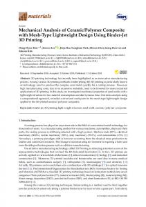
Moreover,  the  CFRP‐phase  model  was  validated  through  the  simplest  manner  of  force  Moreover, the CFRP-phase model was validated through the simplest manner of force generation generation (cutting force and thrust force) comparison. Figure 5 presents the comparative results of  (cutting force and thrust force) comparison. Figure 5 presents the comparative results of predicted predicted and experimentally measured forces versus fiber orientation (θ). It was noticeable that the  and experimentally measured forces versus fiber orientation (θ). It was noticeable that the predicted predicted force magnitudes of both cutting force and thrust force yielded a strong correlation and a  force magnitudes of both cutting force and thrust force yielded a strong correlation and a consistent consistent variation trend with the experimental results gained by Iliescu et al. [28], which confirmed  variation trend with the experimental results gained by Iliescu et al. [28], which confirmed sufficient sufficient credibility of the proposed CFRP‐phase model.  credibility of the proposed CFRP-phase model.

  Figure 5. Comparison of the simulated and experimental force generations in CFRP-phase cutting Figure  5.  Comparison  of  the simulated  and experimental  force  generations  in  CFRP‐phase  cutting  modeling [28]: (a) cutting force; (b) thrust force (cutting condition: vc = 6 m/min, f = 0.2 mm, α = 0˝ ). modeling [28]: (a) cutting force; (b) thrust force (cutting condition: vc = 6 m/min, f = 0.2 mm, α = 0°). 

4. Numerical Results and Discussion

11 hybrid CFRP/Ti cutting are presented with the In this Section, numerical analyses concerning aim of better machining comprehension. Since Ti phase cutting and CFRP phase cutting require different optimal cutting parameters (vc and f ), the cutting conditions used in the FE simulations were selected based on the compromise selection of the optimal parametric range for both the two phases of machining. Special focus was made on the analyses of the cutting process, interface damage formation, and parametric effects on fiber/matrix damage extent. 4.1. Cutting Process Investigation The cutting process of hybrid CFRP/Ti exhibits quite differently from the single-composite and single-metal cutting cases due to the multi-tool-work interaction domains. The disparate natures of each constituent make the chip separation modes more interrelated and coupled governing the bi-material interface consumption (BIC) [37,38]. The interface cutting commonly experienced changeable chip-separation modes and severe transitions of thermo/mechanical responses (e.g., force generation, cutting temperature, strain/stress flow). To reveal the key phenomena controlling CFRP/Ti cutting, the evolution of force generation versus cutting time and also the chip formation progression under fixed cutting conditions of vc = 40 m/min, f = 0.2 mm/rev and θ = 0˝ are presented in Figures 6

single‐metal cutting cases due to the multi‐tool‐work interaction domains. The disparate natures of  The cutting process of hybrid CFRP/Ti exhibits quite differently from the single‐composite and  each  constituent  make  the  chip  separation  modes  more  interrelated  and  coupled  governing  the  single‐metal cutting cases due to the multi‐tool‐work interaction domains. The disparate natures of  bi‐material  interface  consumption  (BIC)  [37,38].  The  interface  cutting  commonly  experienced  each  constituent  make  the  chip  separation  modes  more  interrelated  and  coupled  governing  the  changeable  chip‐separation  modes  and  severe  transitions  of  thermo/mechanical  responses  (e.g.,  bi‐material  interface  consumption  (BIC)  [37,38].  The  interface  cutting  commonly  experienced  force generation, cutting temperature, strain/stress flow). To reveal the key phenomena controlling  Materials 2016, 9,chip‐separation  22 11 of 22 changeable  modes  and  severe  transitions  of  thermo/mechanical  responses  (e.g.,  CFRP/Ti cutting, the evolution of force generation versus cutting time and also the chip formation  force generation, cutting temperature, strain/stress flow). To reveal the key phenomena controlling  progression under fixed cutting conditions of vc = 40 m/min, f = 0.2 mm/rev and θ = 0° are presented  CFRP/Ti cutting, the evolution of force generation versus cutting time and also the chip formation  and 7 respectively. force generations in CFRP/Ti cutting were split into two components, i.e., in  Figures  6  and  7, The respectively.  The  force  generations  in  CFRP/Ti  cutting  were  split  into  two  progression under fixed cutting conditions of vc = 40 m/min, f = 0.2 mm/rev and θ = 0° are presented  the cutting-force component (F ) and the thrust-force component (F ), which signify the tribological c t components, i.e., the cutting‐force component (F c) and the thrust‐force component (F t), which signify  in  Figures  6  and  7,  respectively.  The  force  generations  in  CFRP/Ti  cutting  were  split  into  two  interactions between tool rake and chip surfaces, together with tool together  flank andwith  machined surfaces, the  tribological  interactions  between  tool  rake  and  chip  surfaces,  tool  flank  and  components, i.e., the cutting‐force component (Fc) and the thrust‐force component (Ft), which signify  respectively. It was noticeable that typically three cutting stages referring to the Ti-phase cutting, machined surfaces, respectively. It was noticeable that typically three cutting stages referring to the  the  tribological  interactions  between  tool  rake  and  chip  surfaces,  together  with  tool  flank  and  interface cutting, CFRP-phase could be seen from the force signal variation and the Ti‐phase  cutting,  and interface  cutting,  cutting and  CFRP‐phase  cutting  could  be  seen  from  the  force  signal  machined surfaces, respectively. It was noticeable that typically three cutting stages referring to the  chip-morphology variation and the chip‐morphology evolution.  Ti‐phase  cutting, evolution. interface  cutting,  and  CFRP‐phase  cutting  could  be  seen  from  the  force  signal  variation and the chip‐morphology evolution.  1200

Cutting force

1200

Force generation, F(N) (N/mm) Force generation, F (N) Force generation, FF (N/mm) Force generation,

   

Thrust force Cutting force Thrust force

800 800

Ti-phase cutting

400

Ti-phase cutting

400

0

CFRP-phase cutting CFRP-phase cutting Force fluctuation Force fluctuation

Force fluctuation Force fluctuation

0

Force fluctuation

Force fluctuation

0.000 0.000

0.001 0.002 0.002 0.001 0.002 Cutting time, t0.002 (s) Cutting time, t (s)

0.003 0.003 0.003 0.003

   

Figure 6. Evolution of the force generation versus cutting time when cutting hybrid CFRP/Ti composite  Figure 6. Evolution of the force generation versus cutting time when cutting hybrid CFRP/Ti composite Figure 6. Evolution of the force generation versus cutting time when cutting hybrid CFRP/Ti composite  (v c = 40 m/min, f = 0.2 mm/rev and θ = 0°). ˝ (v(v 40 m/min, f = 0.2 mm/rev and θ = 0 ).  = 40 m/min, f = 0.2 mm/rev and θ = 0°).  c c=

  Figure 7. Chip‐morphology evolution during CFRP/Ti cutting: (a) Ti‐phase cutting; (b) interface cutting;  Figure 7. Chip-morphology evolution during CFRP/Ti cutting: (a) Ti-phase cutting; (b) interface Figure 7. Chip‐morphology evolution during CFRP/Ti cutting: (a) Ti‐phase cutting; (b) interface cutting;  c = 40 m/min, f = 0.2 mm/rev and θ = 0°) (Note: the symbol “S” in the figure  (c) CFRP‐phase cutting (v cutting; (c) CFRP-phase cutting (vc = 40 m/min, f = 0.2 mm/rev and θ = 0˝ ) (Note: the symbol “S” in c = 40 m/min, f = 0.2 mm/rev and θ = 0°) (Note: the symbol “S” in the figure  (c) CFRP‐phase cutting (v represents the von Mises stress and the unit is MPa).  the figure represents the von Mises stress and the unit is MPa). represents the von Mises stress and the unit is MPa). 

As depicted in Figures 6 and 7 when the 13 tool edges initially cut into the Ti phase, material 13 separation occurred through the elastic-plastic deformation mode that controlled the tool-Ti interaction area. The shearing actions arising from the thermo-mechanical coupling effects produced “continuous” chip morphology that flowed on the tool rake face. It should be noted that the Ti-chip morphology exhibited strong sensitivity to the input parameters (cutting parameters and tool geometries) during machining. Since very low cutting speed and positive tool rake angle were used in the current simulation case, the resected chip shape exhibited a more “continuous” rather than a “serrated” appearance. Under the fixed cutting conditions, the machining operation gradually achieved a steady state for which the forces generation approximately attained a stable variation condition. Besides, despite reaching a steady cutting process, high-frequency force fluctuation was also pronounced in Ti-phase cutting as described in Figure 6. The force-generation usually signifies the mechanical-energy consumption of tool-work interactions in cutting and presents a close relation with the inherent properties of the studied workpiece. Since the Ti alloy exhibited ductile behavior and low thermal conductivity, the chip separation typically involved serious thermo-plastic instability and shear localization in the primary cutting zone. Such a phenomenon would promote the quick occurrence of crack initiation and progression dominating the active cutting zones and result in the instability

 

Materials 2016, 9, 22

12 of 22

of the tool-work interaction controlling the chip removal process, as reflected in the cyclic force fluctuations. In addition, when the cutting time (t) approximately exceeded 1.0 ms, the cutting-force component was observed to suffer a gradual reduction. The physical phenomenon could be explained by the decreased uncut Ti-chip thickness contributing to the reduction of force resistance when the tool tended to finalize the Ti-phase cutting. With tool advancement, especially when the cutting edges cut into the interface region, the previously-resected Ti chip adhered on the tool rake face and replaced the tool edges for further chip separation. Due to the transition from tool-Ti interaction to tool-CFRP interaction, the cutting force magnitudes underwent quick drop throughout the interface cutting. In such circumstances, the chip separation mode shifted gradually from plastic-defamation into brittle-fracture, which inevitably resulted in the serious transfer of mechanical/physical loads exerted on the tool-work system. The harsh cutting conditions dominating the CFRP/Ti interface cutting was the key contributor promoting the severe damage formation in the bi-material interface. With further cutting progression, the tool tip cut across the interface region completely and induced a large extent of delamination damage focused on the interface area as shown in the magnified view of Figure 7c. When the tool penetrated into the CFRP phase, material removal took place through successive ruptures aided by the diverse nature and uneven load sharing among the fiber/matrix systems. Since brittle fracture operated as the predominant cutting mode, the resected chip morphology was produced in the form of “discontinuous” shape (especially “dust” like appearance), as illustrated in Figure 7c. Concerning force generation, both the cutting force and thrust force signals were predicted to undergo severe fluctuation and high-frequency variation. However, the mechanisms governing the physical phenomena were disparate. For the cutting force variation, it was induced due to the crack initiation and evolution governing the chip separation process. In contrast, the thrust force fluctuation was mainly attributed to the intense bouncing-back effects on the tool flank surface arising from released carbon fibers in the machined surface [39]. Moreover, when the cutting tool approached the finish of the cutting process, a significant increase of cutting force generation became pronounced as portrayed in Figure 6. This abnormal phenomenon could be explained as follows. When the tool cuts into the CFRP phase, the Ti chip adhered on the tool rake face and replaced the cutting edges for further chip separation. In addition, the produced “dust” like composite chips also caused serious clogging on the head of the Ti chip. Due to these phenomena, the accumulated chip volume inevitably led to a dramatic rise of the cutting resistance, and hence the higher cutting force generation. 4.2. Inspection of Interface Damage Formation In CFRP/Ti cutting, the bi-material interface consumption (BIC) signifies the tremendous mechanical/thermal energy transfer arising from disparate phase cutting, the interrelated chip separation modes, and mixed machining responses controlling the hybrid cutting process. BIC plays a significant role in affecting the final surface quality and subsurface damage formation. The interface cutting can be identified as the weakest region vulnerable to serious damage formation. Figure 8 presents the FE observation of interface damage morphology with OC of CFRP/Ti composite under the cutting conditions of vc = 40 m/min, f = 0.2 mm/rev and θ = 0˝ . It was noticeable that the key characteristic of the interface damage was a “V-shape” like notch damage focused on the CFRP-Ti contact boundary. A large extent of delamination damage became pronounced in both tool-cutting direction (X-direction) and through-thickness direction (Y-direction) as depicted in Figure 8. However, the key manifestation was the severe tearing in the CFRP-phase boundary deviating far from the Ti-phase boundary. The physical phenomena demonstrated that the crack trajectory would experience a quick damage evolution concerning the tool cutting direction during the machining process. The key mechanisms controlling the crack trajectory and evolution in the bi-material interface were strongly influenced by two important factors. The first was the relative fracture toughness arising from the stacked constituents of the bi-material system. It is believed that the crack path prefers to take place nearer the more brittle constituent characterized by lower fracture toughness since it needs less energy

Figure  Figure 8.  8. However,  However, the  the key  key manifestation  manifestation was  was the  the severe  severe tearing  tearing in  in the  the CFRP‐phase  CFRP‐phase boundary  boundary  deviating  deviating far  far from  from the  the Ti‐phase  Ti‐phase boundary.  boundary. The  The physical  physical phenomena  phenomena demonstrated  demonstrated that  that the  the crack  crack  trajectory would experience a quick damage evolution concerning the tool cutting direction during  trajectory would experience a quick damage evolution concerning the tool cutting direction during  the  the machining  machining process.  process. The  The key  key mechanisms  mechanisms controlling  controlling the  the crack  crack trajectory  trajectory and  and evolution  evolution in  in the  the  bi‐material interface  were strongly influenced  by  two  important  factors.  The  first  was  the  relative  bi‐material interface  were strongly influenced  by  two  important  factors.  The  first  was  the  relative  Materials 2016, 9, 22 13 of 22 fracture toughness arising from the stacked constituents of the bi‐material system. It is believed that  fracture toughness arising from the stacked constituents of the bi‐material system. It is believed that  the  the crack  crack path  path prefers  prefers to  to take  take place  place nearer  nearer the  the more  more brittle  brittle constituent  constituent characterized  characterized by  by lower  lower  fracture toughness since it needs less energy to open and propagate the crack damage. In such a case,  to open and propagate the crack damage. In such a case, the preferred crack path occurring in the fracture toughness since it needs less energy to open and propagate the crack damage. In such a case,  the  crack  path  in  CFRP/Ti  interface  should  exhibit  to  CFRP/Ti interface should exhibit more closely to the CFRP-phase boundary due toclosely  its relatively the preferred  preferred  crack  path occurring  occurring  in the  the  CFRP/Ti  interface  should  exhibit more  more  closely  to the  the  CFRP‐phase boundary due to its relatively lower fracture toughness as compared to its counterpart.  lower fracture toughness as compared to its counterpart. Another factor was the specific fracture CFRP‐phase boundary due to its relatively lower fracture toughness as compared to its counterpart.  Another factor was the specific fracture mode encountered along the bi‐material interface. Figure 9  mode encountered along the bi-material interface. Figure 9 shows the schematization of the crack Another factor was the specific fracture mode encountered along the bi‐material interface. Figure 9  shows the schematization of the crack path and fracture modes I and II in cutting. It could be seen  path and fracture modes I and II in cutting. It could be seen that when the tool edges completely shows the schematization of the crack path and fracture modes I and II in cutting. It could be seen  that when the tool edges completely passed through the Ti‐phase boundary, the load path exerting  passed through the Ti-phase boundary, the load path exerting on the bi-material system was uniquely that when the tool edges completely passed through the Ti‐phase boundary, the load path exerting  on the bi‐material system was uniquely applied on the uncut CFRP and interface layers while the  applied on the uncut CFRP and interface layers while the machined Ti-phase surface was deprived on the bi‐material system was uniquely applied on the uncut CFRP and interface layers while the  machined Ti‐phase surface was deprived of load occupation. As such, the cutting load parallel to the  of load occupation. As such, the cutting load parallel to the tool cutting direction together with the machined Ti‐phase surface was deprived of load occupation. As such, the cutting load parallel to the  tool  direction  with  the  perpendicular  to  cutting  would  thrust load perpendicular to the cutting direction would produce mixed modes (fracture tool cutting  cutting  direction together  together  with  the thrust  thrust load  load  perpendicular  to the  the damage cutting direction  direction  would  produce  mixed  damage  modes  (fracture  modes  I  and  II)  on  the  interface  region.  Consequently,   modes I and II) on the interface region. Consequently, it resulted in a sole path evolution of crack produce  mixed  damage  modes  (fracture  modes  I  and  II)  on  the  interface  region.  Consequently,   it  in  path  evolution  of  trajectory  the  cutting  trajectory approaching cutting direction. This inevitably gave to thedirection.   so-called it  resulted  resulted  in  a a  sole  sole the path  evolution  of  crack  crack phenomenon trajectory  approaching  approaching  the rise cutting  direction.   This phenomenon inevitably gave rise to the so‐called “delamination” damage.  “delamination” damage. This phenomenon inevitably gave rise to the so‐called “delamination” damage. 

   Figure 8. FE observation of interface damage when cutting hybrid CFRP/Ti composite (v Figure 8. FE observation of interface damage when cutting hybrid CFRP/Ti composite (vcc = 40 m/min,  40 m/min, Figure 8. FE observation of interface damage when cutting hybrid CFRP/Ti composite (v c=  = 40 m/min,  ˝ f = 0.2 mm/rev and θ = 0°) (Note: the symbol “S” in the figure represents the von Mises stress and the  ff = 0.2 mm/rev and θ = 0°) (Note: the symbol “S” in the figure represents the von Mises stress and the  = 0.2 mm/rev and θ = 0 ) (Note: the symbol “S” in the figure represents the von Mises stress and the unit is MPa).  unit is MPa). unit is MPa). 

   Figure 9. Scheme of (a) crack path in interface region and (b) fracture modes I and II in cutting.  Figure 9. Scheme of (a) crack path in interface region and (b) fracture modes I and II in cutting.  Figure 9. Scheme of (a) crack path in interface region and (b) fracture modes I and II in cutting.

15 To specify the dynamic process of delamination 15 formation and also the affected interface zone (AIZ), nine interface nodes beneath the trimmed plane were selected to characterize their X-direction displacement versus cutting time (t) as shown in Figure 10. Table 8 summarizes the depth beneath the trim plane of the selected interface nodes. The AIZ studied here was devoted to clarifying the actual cutting time that influenced the interface damage formation during the orthogonal cutting process.

To specify the dynamic process of delamination formation and also the affected interface zone  (AIZ),  nine  interface  nodes  beneath  the  trimmed  plane  were  selected  to  characterize  their  X‐direction displacement versus cutting time (t) as shown in Figure 10. Table 8 summarizes the depth  beneath  the  trim  plane  of  the  selected  interface  nodes.  The  AIZ  studied  here  was  devoted  to  clarifying  the  actual  cutting  time  that  influenced  the  interface  damage  formation  during  the  Materials 2016, 9, 22 14 of 22 orthogonal cutting process. 

  Figure 10. Scheme of selected interface nodes in the CFRP/Ti model. Figure 10. Scheme of selected interface nodes in the CFRP/Ti model.  Table 8. Y-displacement from the trim plane of selected nodes in the interface zone. Table 8. Y‐displacement from the trim plane of selected nodes in the interface zone. 

Number of   Depth beneath the Trim Plane  Depth beneath the Number of Node Node  (μm)  Trim Plane (µm) 1  5  1 5 3  40  3 40 5  80  80 5 7  120  120 7 9  160  160 9

Depth beneath the Trim Plane   Number Depth beneath the Number of Node of Node (μm)  Trim Plane (µm) 2  20  2 20 4  60  60 4 6  100 100 6 8  140 140 8 - ‐ 

Figure 11 11 then then  illustrates  X  displacement  evolution  the  selected  interface  nodes  with  Figure illustrates thethe  X displacement evolution of theof  selected interface nodes with respect respect to the cutting time (t) under the fixed cutting conditions of v c = 40 m/min, f = 0.2 mm/rev, and   to the cutting time (t) under the fixed cutting conditions of vc = 40 m/min, f = 0.2 mm/rev, and θ = 0°. It was apparent that the X displacements of the selected interface nodes generally underwent  ˝ θ = 0 . It was apparent that the X displacements of the selected interface nodes generally underwent three variation stages, i.e., the initial variation stage, rapid variation stage, and steady variation stage  three variation stages, i.e., the initial variation stage, rapid variation stage, and steady variation during the total cutting duration (t = 3.0 ms). At the beginning of cutting, all the selected interface  stage during the total cutting duration (t = 3.0 ms). At the beginning of cutting, all the selected nodes  were  predicted  to  suffer  displacement  variation,  which which indicated  that  the  interface nodes were predicted toslow‐rate  suffer slow-rate displacement variation, indicated thatchip  the removal process initially exhibited slight/minor effects on the interface region. However, with the  chip removal process initially exhibited slight/minor effects on the interface region. However, with cutting progression, the machining operation gradually exerted significant influences on the output  the cutting progression, the machining operation gradually exerted significant influences on the responses  of  the of interface  region  with with evidence  that that all all the  to  output responses the interface region evidence theselected  selectedinterface  interfacenodes  nodes began  began to experience high-extent high‐extent displacement displacement  fluctuations fluctuations  and  quickly  enter enter  into into  the the  rapid rapid  variation variation  stage. stage.  experience and quickly The physical phenomena were predicted to take place in the Ti‐phase cutting period approximately  The physical phenomena were predicted to take place in the Ti-phase cutting period approximately at a cutting time of 1.0 ms. Such evidence signified the advent of the affected interface zone (AIZ)  at a cutting time of 1.0 ms. Such evidence signified the advent of the affected interface zone (AIZ) prior  to the the interface-cutting interface‐cutting period period as as illustrated illustrated in in Figure Figure 11. 11. The The occurrence occurrence of of AIZ AIZ commonly commonly  prior to implied  that  the  CFRP/Ti  interface  had  suffered  dramatic  influences  arising  from  the  Ti‐chip  implied that the CFRP/Ti interface had suffered dramatic influences arising from the Ti-chip removal removal  process.  As  depicted  in  Figure  11a,  the  produced  Ti  chip  caused  severe  bending  and  process. As depicted in Figure 11a, the produced Ti chip caused severe bending and inclination effects inclination  effects  on and the also interface  zone  and  also  layer. the  uncut  CFRP‐chip  layer.  The  pronounced  on the interface zone the uncut CFRP-chip The pronounced displacement variation displacement  variation  in  AIZ  strongly  demonstrated  the  appearance  of  serious  detaching  and  in AIZ strongly demonstrated the appearance of serious detaching and separation concerning the separation concerning the interface zone. In addition, the interface nodes located near the trim plane  interface zone. In addition, the interface nodes located near the trim plane typically underwent larger typically underwent larger X displacement compared to their counterparts far away from the trim  X displacement compared to their counterparts far away from the trim plane. The reason might 16 from tool-work interactions. When the cutting be due to the different levels of influences arising time approximately reached 2.0 ms, the X displacements of the selected interface nodes gradually achieved the steady variation state, indicating the diminishing trend of the cutting influences on the interface region. For instance, as shown in Figure 11c, both the deamination lengths in X and Y directions reached their stable values. In such a case, the AIZ could be defined probably at a duration

Materials 2016, 9, 22 

plane.  The  reason  might  be  due  to  the  different  levels  of  influences  arising  from  tool‐work  interactions.  When  the  cutting  time  approximately  reached  2.0  ms,  the  X  displacements  of  the  selected  interface  nodes  gradually  achieved  the  steady  variation  state,  indicating  the  diminishing  Materials 2016, 9, 22 15 of 22 trend of the cutting influences on the interface region. For instance, as shown in Figure 11c, both the  deamination lengths in X and Y directions reached their stable values. In such a case, the AIZ could  of P [1.0, 2.0probably  ms]. Withat regard to the severe displacement occurring the steady variation be t defined  a  duration  of  t ∈ [1.0,  2.0  ms]. fluctuation With  regard  to  the insevere  displacement  state, the reason might be induced as being due to the bouncing-back effects from adjacent CFRP fluctuation occurring in the steady variation state, the reason might be induced as being due to the  elements still affected the local cutting operation. At still  the end of theby  cutting process, all the selected bouncing‐back  effects by from  adjacent  CFRP  elements  affected  the  local  cutting  operation.   interface nodes approached attainment of constant displacements in the X direction except the interface At the end of the cutting process, all the selected interface nodes approached attainment of constant  node 1. The dramatic displacement increase of interface node 1 demonstrated that the node had been displacements in the X direction except the interface node 1. The dramatic displacement increase of  deleted completely from the interface zone. interface node 1 demonstrated that the node had been deleted completely from the interface zone. 

  Figure 11. Displacement in X‐direction of selected interface nodes versus cutting time (t): (a) cutting  Figure 11. Displacement in X-direction of selected interface nodes versus cutting time (t): (a) cutting process at t = 1.17 ms; (b) cutting process at t = 1.58 ms and (c) cutting process at t = 1.85 ms.  process at t = 1.17 ms; (b) cutting process at t = 1.58 ms and (c) cutting process at t = 1.85 ms.

To quantify the delamination extent occurring in the interface zone, three indicators, i.e., D To quantify the delamination extent occurring in the interface zone, three indicators, i.e.,X, D DXY, , and S D  were introduced for evaluation in this study, where D X  signified the delamination length in  DY , and SD were introduced for evaluation in this study, where DX signified the delamination the tool‐cutting direction (X‐direction), D Y denoted the delamination length in the through‐thickness  length in the tool-cutting direction (X-direction), DY denoted the delamination length in the direction  (Y‐direction)  and  S D  implied  the  delamination  area  of  the  damage  zone  as  shown  through-thickness direction (Y-direction) and SD implied the delamination area of the damage zone schematically in Figure 12. The delamination area (S D) was defined as illustrated in Equation (13).  as shown schematically in Figure 12. The delamination area (SD ) was defined as illustrated in

SD  0.5  DX  DY  

Equation (13).

(13) (13)

SD “ 0.5 ˆ DX ˆ DY vc Uncut chip layer

Tool

vc

Tool

Uncut chip layer

Y

Zone of Interest

Y X

Zone of Interest DX

X DX SD

f

SD

f

θ

θ

CFRP

Ti-6Al-4V

CFRP

Ti-6Al-4V

DY

DY

 

Figure 12. Scheme of delamination damage evaluation in CFRP/Ti cutting.  Figure 12. Scheme of delamination damage evaluation in CFRP/Ti cutting.

17 delamination damage versus cutting time (t). Figure 13 presents the evolution of interface The results confirmed that all the delamination indicators (DX , DY and SD ) exhibited similar evolution

Materials 2016, 9, 22  Materials 2016, 9, 22 16 of 22 Figure 13 presents the evolution of interface delamination damage versus cutting time (t). The 

results  confirmed  that  all  the  delamination  indicators  (DX,  DY  and SD)  exhibited  similar  evolution  trends as the X displacements of the selected interface nodes versus cutting time (t) in Figure 11. The  trends as the X displacements of the selected interface nodes versus cutting time (t) in Figure 11. comparison mutually demonstrated the reliability of the two numerical observations. Moreover, as  The comparison mutually demonstrated the reliability of the two numerical observations. Moreover, depicted in Figure 13, from the geometrical consideration, the entire hybrid CFRP/Ti cutting can be  as depicted in Figure 13, from the geometrical consideration, the entire hybrid CFRP/Ti cutting can be divided into three stages referring to (i) Ti‐phase cutting, (ii) interface cutting, and (iii) CFRP‐phase  divided into three stages referring to (i) Ti-phase cutting, (ii) interface cutting, and (iii) CFRP-phase cutting in in terms terms  their  respective  cutting  lengths.  However,  a  category  actually  couldn’t  cutting ofof  their respective cutting lengths. However, such such  a category actually couldn’t reflect reflect  the  real  machining  behavior  of  the  bi‐material  system  due  to  ignorance  of  the  interactive  the real machining behavior of the bi-material system due to ignorance of the interactive cutting cutting influences arising from each‐phase cutting. In reality, the entire hybrid cutting process could  influences arising from each-phase cutting. In reality, the entire hybrid cutting process could be be divided into three basic zones based on the interactive influences of each phase machining.  divided into three basic zones based on the interactive influences of each phase machining. 5500 Dx D X

115

Dy DY

MCFRP/Ti Affected interface zone

SD SD

4500

95

3500

75

Pure Ti-phase cutting MTi

55

Pure CFRP-phase cutting MCFRP

Interface cutting zone

1500

35 Ti-phase cutting zone

15

2500

CFRP-phase cutting zone

500

-5

Delamination area, S (μm2)

Delamination length (μm)

135

-500 0

0.5

1

1.5 2 Cutting time, t (ms)

2.5

3

 

Figure 13. Evolution of delamination damage (DXX,, D DYY and S and SDD) as function of cutting time (t).  ) as function of cutting time (t). Figure 13. Evolution of delamination damage (D

(i) Pure Ti-phase cutting t P [0, 1.0 ms] signifies the cutting period concerning the absolute Ti-phase (i)  Pure  Ti‐phase  cutting  t ∈ [0,  1.0  ms]  signifies  the  cutting  period  concerning  the  absolute  machining with minimum influence affecting the CFRP/Ti interface and the CFRP zone. Such a zone Ti‐phase  machining  with  minimum  influence  affecting  the  CFRP/Ti  interface  and  the  CFRP  zone.  represents the machinability of the single Ti-alloy phase (MTi ). Such a zone represents the machinability of the single Ti‐alloy phase (MTi).  (ii) AIZ cutting t P [1.0, 2.0 ms] denotes the cutting duration concerning the machining variation (ii) AIZ cutting t ∈ [1.0, 2.0 ms] denotes the cutting duration concerning the machining variation  of the bi-material interface arising from Ti-phase cutting and CFRP-phase cutting. Moreover, the AIZ of  the  bi‐material  interface  arising  from  Ti‐phase  cutting  and  CFRP‐phase  cutting.  Moreover,   cutting zone in reality represents the real machinability of the stacked CFRP/Ti material (MCFRP/Ti ). the  AIZ  cutting  zone  in  reality  represents  the  real  machinability  of  the  stacked  CFRP/Ti   (iii) Pure CFRP-phase cutting t P [2.0, 3.0 ms] implies the cutting time concerning the absolute material (M CFRP/Ti).  CFRP-phase machining and reflects the machinability of the standard CFRP phase (MCFRP ). (iii) Pure CFRP‐phase cutting t ∈ [2.0, 3.0 ms] implies the cutting time concerning the absolute  During the pure Ti-phase cutting zone, all DX , DY and SD nearly remained constant values CFRP‐phase machining and reflects the machinability of the standard CFRP phase (M CFRP).  (probably zero values), indicating that no delamination occurred in the interface zone. With the During  the  pure  Ti‐phase  cutting  zone,  all  DX,  DY  and  SD  nearly  remained  constant  values  continuation of the cuttingindicating  process, especially when t reachedoccurred  the AIZ, the threeinterface  delamination (probably  zero  values),  that  no  delamination  in  the  zone. indicators With  the  totally suffered a dramatic increase with elevated cutting time. Such a phenomenon that continuation  of  the  cutting  process,  especially  when  t  reached  the  AIZ,  the  three  signified delamination  the delamination was principally formedwith  at theelevated  AIZ cutting period. Besides, thephenomenon  subsequent indicators  totally damage suffered  a  dramatic  increase  cutting  time.  Such  a  reduction of the delamination indicators in the AIZ might be caused by the bouncing-back effects signified that the delamination damage was principally formed at the AIZ cutting period. Besides,  from adjacent CFRP elements affected by the cutting operation. Moreover, with further increased the  subsequent  reduction  of  the  delamination  indicators  in  the  AIZ  might  be  caused  by  the  t, especially in the purefrom  CFRP-phase cuttingelements  zone, DXaffected  , DY andby  SDthe  gradually reached their steady bouncing‐back  effects  adjacent  CFRP  cutting  operation.  Moreover,  values, which meant that the later cutting process (post CFRP-phase cutting) generated less effect on with further increased t, especially in the pure CFRP‐phase cutting zone, DX, DY and SD gradually  the interface delamination formation. reached their steady values, which meant that the later cutting process (post CFRP‐phase cutting)  Moreover, to inspect the effects of input variables on the AIZ and also on the interface delamination generated less effect on the interface delamination formation.  extent, a parametric study the  was effects  performed by considering various cutting and feed rates. Moreover,  to  inspect  of  input  variables  on  the  AIZ  and speeds also  on  the  interface  Figures 14 and 15 present the acquired results. Note that in Figure 14, the symbol “I” indicates the delamination extent, a parametric study was performed by considering various cutting speeds and  cutting duration of AIZ and the interfacethe  delamination extent (D) wasthat  measured based thesymbol  DY length feed  rates.  Figures  14  and  15  present  acquired  results.  Note  in  Figure  14, on the  “I”  (delamination length in the through-thickness direction (Y-direction)). As can be seen in Figure 14, indicates the cutting duration of AIZ and the interface delamination extent (D) was measured based  both vc and f were found to have significant effects on the AIZ cutting time. Specifically, vc exhibited on the D Y length (delamination length in the through‐thickness direction (Y‐direction)). As can be  aseen  negative impact thevcAIZ impact of f wason  positive. parametric in  Figure  14, on both    and cutting f  were duration found  to while have the significant  effects  the  AIZ Acutting  time.  combination of high v and low f commonly resulted in the lowest AIZ cutting duration. Moreover, c Specifically, vc exhibited a  negative impact  on  the  AIZ  cutting duration  while  the  impact  of  f  was  as is evident in Figure 15, all the examined parametric variables showed pronounced influences on 18

Materials 2016, 9, 22  Materials 2016, 9, 22 17 of 22 positive. A parametric combination of high v c and low f commonly resulted in the lowest AIZ cutting 

positive. A parametric combination of high vc and low f commonly resulted in the lowest AIZ cutting  duration.  Moreover,  as  is  evident  in  Figure  15,  all  the  examined  parametric  variables  showed  pronounced  influences  on extent. the  interface  delamination  The  of i.e., vc  was  found  to  the interface delamination The impact of vc wasextent.  found to be impact  negative, an increase of be  vc negative, i.e., an increase of v c resulted in the reduction of D, while the impact of f was positive. The  resulted in the reduction of D, while the impact of f was positive. The mechanisms controlling the mechanisms controlling the variation phenomena could be associated with their specific influences  variation phenomena could be associated with their specific influences on AIZ. This was because when on  AIZ.  This  was  because  when  vccutting   was  elevated,  typically  a  reduced  cutting  time  of  AIZ  vc was elevated, typically a reduced time of AIZ was achieved as illustrated in Figure 14.was  As achieved  as  illustrated  in  Figure  14.  As  such,  the  decreased  AIZ  inevitably  alleviated  the  damage  such, the decreased AIZ inevitably alleviated the damage extent of induced interface delamination. In extent of induced interface delamination. In contrast, an increase of f usually led to an increased AIZ  contrast, an increase of f usually led to an increased AIZ (as depicted in Figure 14), and hence gave (as depicted in Figure 14), and hence gave rise to a higher extent of interface delamination as shown  rise to a higher extent of interface delamination as shown in Figure 15b. Therefore, from the above in  Figure  Therefore,  from  of the  above delamination, analyses,  for a high minimizing  the  extent  of  interface  analyses, for15b.  minimizing the extent interface cutting speed and a low feed rate delamination, a high cutting speed and a low feed rate are strongly preferred.  are strongly preferred. 7 12 f = 0.05 mm/rev

f = 0.10 mm/rev

f = 0.15 mm/rev

f = 0.20 mm/rev

Total Total tt == 66 ms ms

Total Total tt == 44 ms ms

4 3 2

Total Total tt == 33 ms ms

5

Total Total tt == 12 12 ms ms

Cutting Cutting time, time, tt (ms) (ms)

6

1 10

20 30 Cutting speed, vc(m/min)

40

 

Figure 14. Effects of cutting speed (vccc) and feed rate (f) on cutting duration of AIZ (Note: “Ι” indicates  ) and feed rate (f ) on cutting duration of AIZ (Note: “I” indicates Figure 14. Effects of cutting speed (v the cutting duration of AIZ) (θ = 0˝ ). the cutting duration of AIZ) (θ = 0°).  (b)100 Interface Interface delamiantion, delamiantion, D D ((m m))

Interface Interface delamiantion, delamiantion, D D ((m m))

(a) 120 Interface delamiantion

100

80

10

20 30 Cutting speed, vcc(m/min)

40

Interface delamiantion

80

60

40

0.05

0.10 0.15 Feed rate, f(mm/rev)

0.20

 

Figure 15. Interface delamination extent (D) in function of: (a) cutting speed (v Figure 15. Interface delamination extent (D) in function of: (a) cutting speed (vc )cc) (f = 0.2 mm/rev and   (f = 0.2 mm/rev and ˝ θ = 0°) and (b) feed rate (f) (v θ = 0 ) and (b) feed rate (f ) (vccc = 40 m/min and θ = 0°).  = 40 m/min and θ = 0˝ ).

4.3. Subsurface Damage Study  4.3. Subsurface Damage Study Apart from the severe interface imperfection, the subsurface damage occurring in the composite  Apart from the severe interface imperfection, the subsurface damage occurring in the composite phase is also a particular concern when machining hybrid CFRP/Ti composite. As discussed above,  phase is also a particular concern when machining hybrid CFRP/Ti composite. As discussed above, the the  composite‐phase  damage  takes following place  following  four  types  of  fiber/matrix  i.e.,  fiber  composite-phase damage takes place four types of fiber/matrix failure, i.e.,failures,  fiber compression compression damage, fiber tensile damage, matrix compression damage, and matrix tensile damage.  damage, fiber tensile damage, matrix compression damage, and matrix tensile damage. To inspect the To  inspect composite the  subsurface  damage  resulting  from  the  hybrid  cutting  operation,   subsurface damagecomposite  resulting from the hybrid cutting operation, a parametric analysis was a parametric analysis was performed. The fiber/matrix failure was measured as the largest distance  performed. The fiber/matrix failure was measured as the largest distance from the machined CFRP 19

Materials 2016, 9, 22 Materials 2016, 9, 22  Materials 2016, 9, 22 

18 of 22

from  the  the  machined  CFRP  CFRP  surface  to  to  the  deepest  deepest  fully  fully  damaged  damaged  area,  area,  as  as  shown  shown  schematically  schematically  in  in  from  surface tomachined  the deepest fullysurface  damaged the  area, as shown schematically in Figure 16. The fiber/matrix Figure 16. The fiber/matrix failure extent was predicted and studied versus the fiber orientation (θ)  Figure 16. The fiber/matrix failure extent was predicted and studied versus the fiber orientation (θ)  failure extent was predicted and studied versus the fiber orientation (θ) under the fixed cutting under the fixed cutting conditions of v  = 40 m/min and f = 0.2 mm/rev as depicted in Figure 17. It  under the fixed cutting conditions of v cc = 40 m/min and f = 0.2 mm/rev as depicted in Figure 17. It  conditions of vc = 40 m/min and f = 0.2 mm/rev as depicted in Figure 17. It was noticeable that was noticeable that the θ exhibited significant influence on the evolution of the various fiber/matrix  was noticeable that the θ exhibited significant influence on the evolution of the various fiber/matrix  the θ exhibited significant influence on the evolution of the various types of fiber/matrix damage damages during the chip removal process. The subsurface damage extent increased with elevated θ,  damages during the chip removal process. The subsurface damage extent increased with elevated θ,  during the chip removal process. The subsurface damage extent increased with elevated θ, especially especially the elevation became pronounced when θ was above 60° as depicted in Figure 17. All the  especially the elevation became pronounced when θ was above 60° as depicted in Figure 17. All the  the elevation became pronounced when θ was above 60˝ as depicted in Figure 17. All the damage damage  types  types  tended  to  to  reach  reach  their  their  maximum  extent  extent  at  θ  θ  =  =  90°.  90°.  With  With  θ’s  θ’s  further  further  increase,  increase,  the  the  damage  types tended totended  reach their maximummaximum  extent at θ = 90˝ .at With θ’s further increase, the subsurface subsurface  damage  appeared  to  suffer  a  slight  decrease.  Such  findings  of  θ’s  effect  on  composite  subsurface  damage to appeared  suffer  a  slight  decrease.  Such  of findings  of  θ’s  on  composite  damage appeared suffer a to  slight decrease. Such findings θ’s effect on effect  composite damage damage  agreed  agreed  well  well  with  with  the  the  observations  observations  of  of  Arola  Arola  et  et  al.  al.  [17],  [17],  and  and  Wang  Wang  and  and  Zhang  Zhang  [39]  [39]  when  when  damage  agreed well with the observations of Arola et al. [17], and Wang and Zhang [39] when cutting CFRP cutting CFRP laminates. The mechanisms controlling the mentioned phenomena could be attributed  cutting CFRP laminates. The mechanisms controlling the mentioned phenomena could be attributed  laminates. The mechanisms controlling the mentioned phenomena could be attributed to the change to  the  change  change  of  of  failure  failure  modes  modes  from  from  bending  bending  and  crushing  crushing  in  case  of  of  θ  θ  =  =  0°  0°  to  to  a  a  fracture  fracture  by  by  to  the  of failure modes from bending and crushing inand  case of θ = 0˝in tocase  a fracture by compression and compression and interfacial‐shearing mode for positive fiber orientation (0°