of testing as many sub-ice shelf circulation models as possible, the aim being to .... The steel hose is used to provide weight to keep the drill hose vertical. ... (e) Cargo ready to be flown to Site 5, with the Site 4 Argos transmitter in ...... depth-averaged equations of continuity and motion in spherical polar coordinates that.
TIDAL CURRENTS AND VERTICAL MIXING PROCESSES BENEATH FILCHNER-RONNE ICE SHELF
Keith Makinson BEng (Hons)
A thesis submitted in partial fulfilment of the requirements of the Open University for the degree of Doctor of Philosophy
March 2002
British Antarctic Survey, Natural Environment Research Council, Cambridge, United Kingdom
-ii-
Abstract Oceanographic measurements have been undertaken at sites on Filchner-Ronne Ice Shelf using hot-water drilled holes allowing conductivity-temperature-depth profiling and the deployment of instrument moorings. The data show that Western Shelf Water enters the sub-ice shelf cavity and occupies the lower portion of the water column. This is the water that provides the external heat necessary for melting within the sub-ice shelf cavity. A depth–averaged tidal model of the region has been used to show that in areas with shallow water and large topographic gradients, tidal oscillations with peak velocities up to 1 m s-1 play a significant role in the vertical mixing and transport of water masses. The estimated energy dissipation beneath Filchner-Ronne Ice Shelf resulting from surface friction is 25 GW, approximately 1% of the world’s total tidal dissipation. The model indicates that Lagrangian tidal residual currents have fluxes of up to 250,000 m3 s-1, and speeds of over 5 cm s-1 along the ice front, with over 350,000 m3 s-1 being exchanged between the sub–ice shelf cavity and adjacent continental shelf. These currents are particularly efficient in ventilating the sub–ice shelf cavity within 150 km of Ronne Ice Front. Furthermore, a one-dimensional turbulence closure ocean model has been applied to this sub-ice shelf environment which significantly lies near the critical latitude for the semi-diurnal tide. Here, the Coriolis frequency equals the tidal frequency, resulting in a strong depth dependent tidal current and thick boundary layers. Both the model and observations show that stratification significantly affects how the shape of the tidal current ellipse varies with depth. The model also shows that vertical mixing and basal melting are sensitive to tidal ellipse polarization with anticlockwise rotating tidal currents maintaining the highest melt rates. This sensitivity is due, in large part, to the proximity of the critical latitude.
-iii-
-iv-
Table of Contents Table of figures . . . . . . . . . . . . . . . . . . . . . . . . . . . . . . . . . . . . . . . . . . . . . . . . . . . . . . . xi Table of tables . . . . . . . . . . . . . . . . . . . . . . . . . . . . . . . . . . . . . . . . . . . . . . . . . . . . . . . . xv Acronyms and Abbreviations . . . . . . . . . . . . . . . . . . . . . . . . . . . . . . . . . . . . . . . . . . . xvii List of accompanying material . . . . . . . . . . . . . . . . . . . . . . . . . . . . . . . . . . . . . . . . . . xix Acknowledgements . . . . . . . . . . . . . . . . . . . . . . . . . . . . . . . . . . . . . . . . . . . . . . . . . . . xxi Declaration . . . . . . . . . . . . . . . . . . . . . . . . . . . . . . . . . . . . . . . . . . . . . . . . . . . . . . . . xxiii CHAPTER 1 Introduction 1.1 Aims and scope of the thesis . . . . . . . . . . . . . . . . . . . . . . . . . . . . . . . . . . . . . 1 1.1.1 Problems to be addressed . . . . . . . . . . . . . . . . . . . . . . . . . . . . . . . . 1 1.1.2 Outline of thesis . . . . . . . . . . . . . . . . . . . . . . . . . . . . . . . . . . . . . . . 2 1.2 Ice shelves . . . . . . . . . . . . . . . . . . . . . . . . . . . . . . . . . . . . . . . . . . . . . . . . . . . 3 1.3 Oceanography of the Southern Ocean . . . . . . . . . . . . . . . . . . . . . . . . . . . . . 3 1.4 Oceanography of the Weddell Sea . . . . . . . . . . . . . . . . . . . . . . . . . . . . . . . . 7 1.5 Filchner-Ronne Ice Shelf . . . . . . . . . . . . . . . . . . . . . . . . . . . . . . . . . . . . . . 10 1.6 Ice-ocean interactions . . . . . . . . . . . . . . . . . . . . . . . . . . . . . . . . . . . . . . . . . 13 1.7 Sub-ice shelf circulation . . . . . . . . . . . . . . . . . . . . . . . . . . . . . . . . . . . . . . . 14 1.7.1 Observations . . . . . . . . . . . . . . . . . . . . . . . . . . . . . . . . . . . . . . . . 14 1.7.2 Numerical models . . . . . . . . . . . . . . . . . . . . . . . . . . . . . . . . . . . . 16 1.8 Ocean tides . . . . . . . . . . . . . . . . . . . . . . . . . . . . . . . . . . . . . . . . . . . . . . . . . 21 1.9 References . . . . . . . . . . . . . . . . . . . . . . . . . . . . . . . . . . . . . . . . . . . . . . . . . . 23 CHAPTER 2 Field Work on Filchner-Ronne Ice Shelf 2.1 Introduction . . . . . . . . . . . . . . . . . . . . . . . . . . . . . . . . . . . . . . . . . . . . . . . . . 27 2.1.1 History of sub-ice shelf oceanography . . . . . . . . . . . . . . . . . . . . 27 2.1.2 Aims of fieldwork . . . . . . . . . . . . . . . . . . . . . . . . . . . . . . . . . . . . 29 2.2 Gaining access - Hot water drilling 1998/99 . . . . . . . . . . . . . . . . . . . . . . . 29 2.2.1 Logistical constrains and site locations . . . . . . . . . . . . . . . . . . . . 29 2.2.2 Local seismic surveys . . . . . . . . . . . . . . . . . . . . . . . . . . . . . . . . . 31 2.2.3 Drilling system description . . . . . . . . . . . . . . . . . . . . . . . . . . . . . 33 2.2.4 Mode of operation . . . . . . . . . . . . . . . . . . . . . . . . . . . . . . . . . . . . 37 -v-
2.2.5 Determination of drilling speeds . . . . . . . . . . . . . . . . . . . . . . . . . 38 2.3 Sub-ice shelf oceanographic instruments . . . . . . . . . . . . . . . . . . . . . . . . . 40 2.3.1 CTD profiler . . . . . . . . . . . . . . . . . . . . . . . . . . . . . . . . . . . . . . . . 40 2.3.2 Thermistor cable . . . . . . . . . . . . . . . . . . . . . . . . . . . . . . . . . . . . . 41 2.3.3 Conductivity-temperature-pressure units and current meters . . . 42 2.3.4 Instrument calibrations (temperature and salinity) . . . . . . . . . . . 44 2.4 Field data . . . . . . . . . . . . . . . . . . . . . . . . . . . . . . . . . . . . . . . . . . . . . . . . . . 46 2.4.1 CTD profiles . . . . . . . . . . . . . . . . . . . . . . . . . . . . . . . . . . . . . . . . 46 2.4.2 Thermistor cable . . . . . . . . . . . . . . . . . . . . . . . . . . . . . . . . . . . . . 49 2.4.3 CTP mooring data . . . . . . . . . . . . . . . . . . . . . . . . . . . . . . . . . . . . 49 2.4.4 Current meter mooring data . . . . . . . . . . . . . . . . . . . . . . . . . . . . 49 2.5 References . . . . . . . . . . . . . . . . . . . . . . . . . . . . . . . . . . . . . . . . . . . . . . . . . 54 CHAPTER 3 Two-Dimensional Barotropic Tidal Model 3.1 Introduction . . . . . . . . . . . . . . . . . . . . . . . . . . . . . . . . . . . . . . . . . . . . . . . . 57 3.2 Numerical tidal model . . . . . . . . . . . . . . . . . . . . . . . . . . . . . . . . . . . . . . . . 58 3.2.1 Governing equations . . . . . . . . . . . . . . . . . . . . . . . . . . . . . . . . . . 58 3.2.2 Model domain . . . . . . . . . . . . . . . . . . . . . . . . . . . . . . . . . . . . . . . 60 3.2.2.1 Bathymetry . . . . . . . . . . . . . . . . . . . . . . . . . . . . . . . . . . 61 3.2.2.2 Ice shelf thickness . . . . . . . . . . . . . . . . . . . . . . . . . . . . 62 3.2.2.3 Sub-ice shelf cavity . . . . . . . . . . . . . . . . . . . . . . . . . . . 63 3.2.3 Model forcing . . . . . . . . . . . . . . . . . . . . . . . . . . . . . . . . . . . . . . . 63 3.3 Analysis of tidal data . . . . . . . . . . . . . . . . . . . . . . . . . . . . . . . . . . . . . . . . . 64 3.3.1 Tidal record length . . . . . . . . . . . . . . . . . . . . . . . . . . . . . . . . . . . 64 3.3.2 Tidal ellipse parameterization . . . . . . . . . . . . . . . . . . . . . . . . . . . 65 3.4 Model validation using elevation data . . . . . . . . . . . . . . . . . . . . . . . . . . . . 67 3.5 References . . . . . . . . . . . . . . . . . . . . . . . . . . . . . . . . . . . . . . . . . . . . . . . . . 70 CHAPTER 4 Southern Weddell Sea Tidal Currents and Vertical Mixing 4.1 Introduction . . . . . . . . . . . . . . . . . . . . . . . . . . . . . . . . . . . . . . . . . . . . . . . . 73 4.2 Model results . . . . . . . . . . . . . . . . . . . . . . . . . . . . . . . . . . . . . . . . . . . . . . . 74 4.2.1 Tidal current ellipses . . . . . . . . . . . . . . . . . . . . . . . . . . . . . . . . . . 74 4.2.2 Tidal shore lead . . . . . . . . . . . . . . . . . . . . . . . . . . . . . . . . . . . . . . 78 4.3 Field data . . . . . . . . . . . . . . . . . . . . . . . . . . . . . . . . . . . . . . . . . . . . . . . . . . 80 -vi-
4.3.1 Weddell Sea current meter records . . . . . . . . . . . . . . . . . . . . . . . 80 4.3.2 Ice front current meter records . . . . . . . . . . . . . . . . . . . . . . . . . . . 83 4.3.3 Sub-ice shelf current meter records . . . . . . . . . . . . . . . . . . . . . . . 85 4.3.4 Proxy current data . . . . . . . . . . . . . . . . . . . . . . . . . . . . . . . . . . . . 87 4.3.5 Accuracy of tidal model . . . . . . . . . . . . . . . . . . . . . . . . . . . . . . . . 88 4.4 Tidal energy and vertical mixing . . . . . . . . . . . . . . . . . . . . . . . . . . . . . . . . 89 4.4.1 Mean water speed . . . . . . . . . . . . . . . . . . . . . . . . . . . . . . . . . . . . 89 4.4.2 Tidal energy flux . . . . . . . . . . . . . . . . . . . . . . . . . . . . . . . . . . . . . 90 4.4.3 Tidal dissipation . . . . . . . . . . . . . . . . . . . . . . . . . . . . . . . . . . . . . . 90 4.4.4 Estimated basal melt rates . . . . . . . . . . . . . . . . . . . . . . . . . . . . . . 92 4.4.5 Observed melt rates . . . . . . . . . . . . . . . . . . . . . . . . . . . . . . . . . . . 94 4.5 Summary and conclusions . . . . . . . . . . . . . . . . . . . . . . . . . . . . . . . . . . . . . 95 4.6 References . . . . . . . . . . . . . . . . . . . . . . . . . . . . . . . . . . . . . . . . . . . . . . . . . . 97 CHAPTER 5 Southern Weddell Sea Residual Tidal Currents 5.1 Introduction . . . . . . . . . . . . . . . . . . . . . . . . . . . . . . . . . . . . . . . . . . . . . . . . 101 5.2 Eulerian residual currents . . . . . . . . . . . . . . . . . . . . . . . . . . . . . . . . . . . . . 104 5.2.1 Model results . . . . . . . . . . . . . . . . . . . . . . . . . . . . . . . . . . . . . . . 105 5.2.2 Field data . . . . . . . . . . . . . . . . . . . . . . . . . . . . . . . . . . . . . . . . . . 107 5.3 Lagrangian residual currents . . . . . . . . . . . . . . . . . . . . . . . . . . . . . . . . . . . 110 5.3.1 Eastern Ronne Ice Front . . . . . . . . . . . . . . . . . . . . . . . . . . . . . . . 114 5.3.2 Western Ronne Ice Font . . . . . . . . . . . . . . . . . . . . . . . . . . . . . . . 115 5.3.3 Continental Shelf . . . . . . . . . . . . . . . . . . . . . . . . . . . . . . . . . . . . 116 5.3.4 Ice shelf cavity . . . . . . . . . . . . . . . . . . . . . . . . . . . . . . . . . . . . . . 117 5.4 Impact on hydrography and ice shelf morphology . . . . . . . . . . . . . . . . . . 119 5.4.1 Tidal oscillations and mixing . . . . . . . . . . . . . . . . . . . . . . . . . . . 119 5.4.2 Residual currents . . . . . . . . . . . . . . . . . . . . . . . . . . . . . . . . . . . . 120 5.4.3 Ice shelf cavity outflows . . . . . . . . . . . . . . . . . . . . . . . . . . . . . . 120 5.4.4 Ice shelf cavity inflows . . . . . . . . . . . . . . . . . . . . . . . . . . . . . . . 123 5.4.5 Modified Weddell Deep Water intrusion . . . . . . . . . . . . . . . . . . 123 5.4.6 Contribution of residual currents to mass transport . . . . . . . . . . 124 5.5 Summary and conclusions . . . . . . . . . . . . . . . . . . . . . . . . . . . . . . . . . . . . 125 5.6 References . . . . . . . . . . . . . . . . . . . . . . . . . . . . . . . . . . . . . . . . . . . . . . . . . 127 -vii-
CHAPTER 6 One-Dimensional Vertical Mixing Model 6.1 Introduction . . . . . . . . . . . . . . . . . . . . . . . . . . . . . . . . . . . . . . . . . . . . . . . 129 6.2 Mean flow equations . . . . . . . . . . . . . . . . . . . . . . . . . . . . . . . . . . . . . . . . 133 6.2.1 Transport of mass . . . . . . . . . . . . . . . . . . . . . . . . . . . . . . . . . . . 133 6.2.2 Surface forcing . . . . . . . . . . . . . . . . . . . . . . . . . . . . . . . . . . . . . 134 6.2.3 Boundary conditions . . . . . . . . . . . . . . . . . . . . . . . . . . . . . . . . . 135 6.2.3.1 Seabed . . . . . . . . . . . . . . . . . . . . . . . . . . . . . . . . . . . . 136 6.2.3.2 Ice shelf base . . . . . . . . . . . . . . . . . . . . . . . . . . . . . . . 137 6.3 Turbulence model . . . . . . . . . . . . . . . . . . . . . . . . . . . . . . . . . . . . . . . . . . 137 6.3.1 Stability functions . . . . . . . . . . . . . . . . . . . . . . . . . . . . . . . . . . . 137 6.3.2 Mellor and Yamada level 2.5 turbulent closure equations . . . . 139 6.4 Water column properties . . . . . . . . . . . . . . . . . . . . . . . . . . . . . . . . . . . . . 140 6.4.1 Vertical diffusion . . . . . . . . . . . . . . . . . . . . . . . . . . . . . . . . . . . 140 6.4.2 Equation of state for seawater . . . . . . . . . . . . . . . . . . . . . . . . . . 140 6.4.3 Temperature and salinity transfer coefficients . . . . . . . . . . . . . 140 6.4.4 Basal melting and freezing point of seawater . . . . . . . . . . . . . . 141 6.4.5 Mixing water masses . . . . . . . . . . . . . . . . . . . . . . . . . . . . . . . . 142 6.5 Internal wave activity . . . . . . . . . . . . . . . . . . . . . . . . . . . . . . . . . . . . . . . . 142 6.5.1 Mellor parameter . . . . . . . . . . . . . . . . . . . . . . . . . . . . . . . . . . . . 143 6.5.2 Kantha and Clayson parameter . . . . . . . . . . . . . . . . . . . . . . . . . 143 6.6 Model structure . . . . . . . . . . . . . . . . . . . . . . . . . . . . . . . . . . . . . . . . . . . . 144 6.7 Model test cases . . . . . . . . . . . . . . . . . . . . . . . . . . . . . . . . . . . . . . . . . . . . 146 6.7.1 Surface stress . . . . . . . . . . . . . . . . . . . . . . . . . . . . . . . . . . . . . . 146 6.7.2 Pressure gradient . . . . . . . . . . . . . . . . . . . . . . . . . . . . . . . . . . . . 147 6.7.3 Surface mixed layer growth . . . . . . . . . . . . . . . . . . . . . . . . . . . 147 6.6.4 Gade line mixing . . . . . . . . . . . . . . . . . . . . . . . . . . . . . . . . . . . . 147 6.7.5 Distribution of turbulent kinetic energy . . . . . . . . . . . . . . . . . . 149 6.8 References . . . . . . . . . . . . . . . . . . . . . . . . . . . . . . . . . . . . . . . . . . . . . . . . 152 CHAPTER 7 Application of Vertical Mixing Model to the Cavity Beneath FRIS 7.1 Introduction . . . . . . . . . . . . . . . . . . . . . . . . . . . . . . . . . . . . . . . . . . . . . . . 155 7.1.1 Ellipse polarization . . . . . . . . . . . . . . . . . . . . . . . . . . . . . . . . . . 156 7.1.2 Critical latitude . . . . . . . . . . . . . . . . . . . . . . . . . . . . . . . . . . . . . 158 -viii-
7.1.2.1 Northern Hemisphere . . . . . . . . . . . . . . . . . . . . . . . . . 158 7.1.2.2 Southern Hemisphere . . . . . . . . . . . . . . . . . . . . . . . . . 162 7.1.3 Stratification . . . . . . . . . . . . . . . . . . . . . . . . . . . . . . . . . . . . . . . . 162 7.2 Model results for sub-ice shelf mooring sites . . . . . . . . . . . . . . . . . . . . . . 163 7.2.1 Model configuration . . . . . . . . . . . . . . . . . . . . . . . . . . . . . . . . . . 163 7.2.2 Site 3 . . . . . . . . . . . . . . . . . . . . . . . . . . . . . . . . . . . . . . . . . . . . . 165 7.2.3 Site 4 . . . . . . . . . . . . . . . . . . . . . . . . . . . . . . . . . . . . . . . . . . . . . 169 7.2.4 Site 5 . . . . . . . . . . . . . . . . . . . . . . . . . . . . . . . . . . . . . . . . . . . . . 170 7.3 Model results for a sub-ice shelf cavity . . . . . . . . . . . . . . . . . . . . . . . . . . 172 7.3.1 Model configuration . . . . . . . . . . . . . . . . . . . . . . . . . . . . . . . . . . 172 7.3.2 Tidal current profiles in a homogeneous sea . . . . . . . . . . . . . . . 173 7.3.3 Tidal current profiles in a stratified sea . . . . . . . . . . . . . . . . . . . 176 7.3.4 Southern Weddell Sea current profiles . . . . . . . . . . . . . . . . . . . 178 7.3.5 Effects of ellipse polarization . . . . . . . . . . . . . . . . . . . . . . . . . . 182 7.4 Application to FRIS . . . . . . . . . . . . . . . . . . . . . . . . . . . . . . . . . . . . . . . . . 184 7.4.1 Polarization -1.0 to -0.3 . . . . . . . . . . . . . . . . . . . . . . . . . . . . . . . 187 7.4.2 Polarization -0.3 to 0.3 . . . . . . . . . . . . . . . . . . . . . . . . . . . . . . . . 189 7.4.3 Polarization 0.3 to 1.0 . . . . . . . . . . . . . . . . . . . . . . . . . . . . . . . . 190 7.5 Summary and conclusions . . . . . . . . . . . . . . . . . . . . . . . . . . . . . . . . . . . . 192 7.6 References . . . . . . . . . . . . . . . . . . . . . . . . . . . . . . . . . . . . . . . . . . . . . . . . . 194 CHAPTER 8 General summary 8.1 Summary of described work . . . . . . . . . . . . . . . . . . . . . . . . . . . . . . . . . . . 197 8.2 What has been learnt from this study? . . . . . . . . . . . . . . . . . . . . . . . . . . . 201 8.3 Future work . . . . . . . . . . . . . . . . . . . . . . . . . . . . . . . . . . . . . . . . . . . . . . . . 204 Appendix A.1 Surface forcing functions . . . . . . . . . . . . . . . . . . . . . . . . . . . . . . . . . . . . . 207 A.2 References . . . . . . . . . . . . . . . . . . . . . . . . . . . . . . . . . . . . . . . . . . . . . . . . 208
-ix-
-x-
Table of Figures Figure 1.1
Map of Antarctica . . . . . . . . . . . . . . . . . . . . . . . . . . . . . . . . . . . . . . . . . . 4
Figure 1.2
Schematic map showing Southern Ocean Circulation . . . . . . . . . . . . . . 4
Figure 1.3
Seasonal changes in sea ice cover around Antarctica . . . . . . . . . . . . . . . 6
Figure 1.4
Global distribution of deep water and bottom water masses . . . . . . . . . 6
Figure 1.5
Schematic showing the water mass characteristics of the Weddell Sea
Figure 1.6
Map of Filchner-Ronne Ice Shelf . . . . . . . . . . . . . . . . . . . . . . . . . . . . . 12
Figure 1.7
Map showing the bathymetry in the area of Filchner-Ronne Ice Shelf 12
Figure 1.8
Photograph of a green ice berg in Weddell Sea . . . . . . . . . . . . . . . . . . 15
Figure 1.9
Section of potential temperature along Filchner-Ronne Ice Front . . . . 19
Figure 1.10
Schematic of the circulation beneath Filchner-Ronne Ice Shelf . . . . . . 19
Figure 1.11
Modelled circulation beneath Filchner-Ronne Ice Shelf . . . . . . . . . . . 20
Figure 2.1
Location map showing logistics routes . . . . . . . . . . . . . . . . . . . . . . . . . 30
Figure 2.2
Bathymetry and ice shelf topography around drill sites . . . . . . . . . . . . 32
Figure 2.3
Block diagram of hot water drilling system . . . . . . . . . . . . . . . . . . . . . 34
Figure 2.4
Photographs of hot water drilling system . . . . . . . . . . . . . . . . . . . . . . . 36
Figure 2.5
Plots of drill water temperature, hole diameter and freezing rates . . . . 39
Figure 2.6
Photographs of sub-ice shelf oceanographic instruments . . . . . . . . . . . 43
Figure 2.7
Schematic of oceanographic instrument calibration facility . . . . . . . . . 45
Figure 2.8
Profiles of potential temperature and salinity at sites 3, 4 and 5 . . . . . 47
Figure 2.9a
Schematic of oceanographic mooring at Site 3 . . . . . . . . . . . . . . . . . . 50
9
Figure 2.9b,c Schematic of oceanographic mooring at sites 4 and 5 . . . . . . . . . . . . . 51 Figure 2.10
Current meter records from sites 3, 4 and 5 . . . . . . . . . . . . . . . . . . . . . 52
Figure 3.1
Schematic showing various depths and elevations used by tidal model 59
Figure 3.2
Map of the tidal model domain and bathymetry . . . . . . . . . . . . . . . . . . 61
Figure 3.3
Schematic of parameters of tidal ellipse . . . . . . . . . . . . . . . . . . . . . . . . 65
Figure 3.4
Comparison of tidal elevation data . . . . . . . . . . . . . . . . . . . . . . . . . . . . 68
Figure 3.5
Map of modelled tidal elevations and phase . . . . . . . . . . . . . . . . . . . . 69
Figure 4.1a,b Modelled Q1 and O1 tidal ellipses . . . . . . . . . . . . . . . . . . . . . . . . . . . . . 75 -xi-
Figure 4.1c,d Modelled K1 and N2 tidal ellipses . . . . . . . . . . . . . . . . . . . . . . . . . . . . 76 Figure 4.1e,f Modelled M2 and S2 tidal ellipses . . . . . . . . . . . . . . . . . . . . . . . . . . . . 77 Figure 4.2
Modelled shore lead area along Ronne Ice Front . . . . . . . . . . . . . . . . 79
Figure 4.3
Map of model domain and current meter locations . . . . . . . . . . . . . . 79
Figure 4.4
Tidal ellipses for shelf break and ice front moorings . . . . . . . . . . . . . 81
Figure 4.5
Tidal ellipses for ice front and sub-ice shelf moorings . . . . . . . . . . . . 84
Figure 4.6
Time series from Site 2 thermistor cable . . . . . . . . . . . . . . . . . . . . . . . 86
Figure 4.7
Average RMS water speeds over model domain . . . . . . . . . . . . . . . . 91
Figure 4.8
Average tidal energy flux vectors over model domain . . . . . . . . . . . . 91
Figure 4.9
Average tidal dissipation over model domain . . . . . . . . . . . . . . . . . . . 93
Figure 4.10
Minimum basal melt rate to maintain stratification . . . . . . . . . . . . . . . 93
Figure 5.1
Schematics showing ice front processes . . . . . . . . . . . . . . . . . . . . . . 103
Figure 5.2
Maximum tidal excursion just offshore of Ronne Ice Front . . . . . . . 106
Figure 5.3
Eulerian residual current vectors over the model domain . . . . . . . . 107
Figure 5.4
Lagrangian tracer trajectories at Ronne Ice Front . . . . . . . . . . . . . . 111
Figure 5.5
Lagrangian residual tidal currents over model domain . . . . . . . . . . . 112
Figure 5.6
A section perpendicular to Ronne Ice Front showing residual flow . 113
Figure 5.7
Lagrangian residual trajectories over the Berkner Shelf region . . . . 114
Figure 5.8
Lagrangian residual trajectories over western Ronne Ice Front . . . . 116
Figure 5.9
Oceanographic sections and Lagrangian flow along ice front region 121
Figure 6.1
Schematics of the subdivision of sea bed boundary layer . . . . . . . . . 135
Figure 6.2
Position of model layer boundaries from sea bed . . . . . . . . . . . . . . . 145
Figure 6.3
A flow diagram of vertical mixing model . . . . . . . . . . . . . . . . . . . . . 145
Figure 6.4
Simulations of open channel flow . . . . . . . . . . . . . . . . . . . . . . . . . . . 148
Figure 6.5
Development of the mixed layer depth . . . . . . . . . . . . . . . . . . . . . . . 148
Figure 6.6
Plots and time series of TKE and dissipation . . . . . . . . . . . . . . . . . . 150
Figure 7.1
Contour plot of the amplitude of the M2 rotary components . . . . . . . 159
Figure 7.2
Contour plot of the amplitude of the S2 rotary components . . . . . . . 160
Figure 7.3
Contour plot of the M2 and S2 ellipse polarizations . . . . . . . . . . . . . . 161
-xii-
Figure 7.4
Contours of clockwise component of M2 around the critical latitude . 164
Figure 7.5
Mean depth profiles of the M2 rotary components near critical latitude164
Figure 7.6
Plot of observed potential temperature at Site 3 . . . . . . . . . . . . . . . . . 165
Figure 7.7
Hourly melt rate at Site 3 over a two-year period . . . . . . . . . . . . . . . 168
Figure 7.8
Smoothed Site 3 current speed record and thermistor temperatures . . 168
Figure 7.9
Plot of observed potential temperature at Site 4 . . . . . . . . . . . . . . . . . 170
Figure 7.10
Water column property profiles at Site 5 . . . . . . . . . . . . . . . . . . . . . . 171
Figure 7.11
Vertical structure of the M2 rotary components beneath an ice shelf
Figure 7.12
The amplitude of the M2 and S2 anticlockwise component
Figure 7.13
The vertical structure of the M2 rotary components during melting . 177
Figure 7.14
Seasonal variation of the M2 rotary components at FR6 . . . . . . . . . . 180
Figure 7.15
Profiles of the M2 rotary components at FR6 . . . . . . . . . . . . . . . . . . . 180
Figure 7.16
Profiles of the M2 rotary components at FR5, R2 and FR3 . . . . . . . . 181
Figure 7.17
Modelled pycnocline depth after 10 M2 cycles of melting . . . . . . . . . 183
Figure 7.18
Contoured pycnocline depth after 10 M2 cycles of melting . . . . . . . . 185
Figure 7.19
Dependance of melt rate on depth averaged rotary components . . . . 185
Figure 7.20
Profiles of model parameters during melting and mixing . . . . . . . . . . 188
Figure 7.21
Pycnocline formation and erosion beneath an ice shelf . . . . . . . . . . . 191
Figure 8.1
Modelled M2 tidal ellipses and polarization . . . . . . . . . . . . . . . . . . . . 199
Figure 8.2
Lagrangian residual tidal currents over model domain . . . . . . . . . . . . 200
Figure 8.3
Areas of vigorous mixing beneath Filchner-Ronne Ice Shelf . . . . . . . 200
Figure 8.4
Modelled pycnocline depth after 10 M2 cycles of melting . . . . . . . . . 202
Figure 8.5
Profiles of the M2 rotary components at FR6 . . . . . . . . . . . . . . . . . . . 202
-xiii-
174
. . . . . . . 175
-xiv-
Table of tables Table 3.1
Principal harmonic components . . . . . . . . . . . . . . . . . . . . . . . . . . . . . . 64
Table 4.1
Schematic map showing Southern Ocean Circulation . . . . . . . . . . . . . 82
-xv-
-xvi-
Acronyms and Abbreviations AABW
Antarctic Bottom Water
ACC
Antarctic Circumpolar Current
AWI
Alfred-Wegener-Institute
BAS
British Antarctic Survey
CFL
Courant-Friedrichs-Lewy
CMR
Christian Michelsen Research
CTD
Conductivity-Temperature-Depth
CTP
Conductivity-Temperature-Pressure
DBDB5
Digital Bathymetric Data Base 5
ESW
Eastern Shelf Water
FRIS
Filchner-Ronne Ice Shelf
GEBCO
General Bathymetric Chart of the Oceans
HSSW
High Salinity Shelf Water
HWD
Hot Water Drill
ISW
Ice Shelf Water
IW
Internal Wave
KPP
K-Profile Parameterization
MICOM
Miami Iso-Pycnic Coordinate Model
MWDW
Modified Weddell Deep Water
MY
Mellor-Yamada
SI
Shear Instability
SPRT
Standard Platinum Resistance Thermometer
TKE
Turbulent Kinetic Energy
WDW
Weddell Deep Water / Warm Deep Water
WSBW
Weddell Sea Bottom Water
WSDW
Weddell Sea Deep Water
WSW
Western Shelf Water
WW
Winter Water
-xvii-
-xviii-
List of accompanying material Makinson, K. and K. W. Nicholls. Modeling tidal currents beneath Filchner-Ronne Ice Shelf and on the adjacent continental shelf: their effect on mixing and transport. Journal of Geophysical Research, 104(C6): 13449-13465, 1999. (Reprint)
Makinson, K. Modeling tidal current profiles and vertical mixing beneath Filchner-Ronne Ice Shelf, Antarctica. Journal of Physical Oceanography, 32(1), 202-215, 2002. (Reprint)
-xix-
-xx-
Acknowledgements I would like to thank the many colleagues who have offered help and encouragement throughout the course of the work presented in this thesis and I wish to thank the following: My supervisors Dr Keith Nicholls and Dr Grant Bigg who provided friendly and expert guidance whenever it was required. I would particularly like to thank Keith Nicholls who initially encouraged me into the world of tides and numerical modelling. The members of the group: Chris Doake, Adrian Jenkins, Lars Semdsrud, David Vaughan and Andy Wood who have reviewed and commented on various chapters or papers associated with this thesis. The fieldwork described in this thesis was very much a team effort and was successfully carried out with the assistance of Steve Hinde, Mark Johnson, Dr Keith Nicholls and Dr Svein Østerhus. Also, to the support staff at Halley and Rothera stations, especially the Air Unit for all their efforts in deploying the team members and vast amounts of equipment and fuel. The work presented in this thesis has been undertaken whilst I have been an employee of British Antarctic Survey. I am grateful to BAS for providing the facilities and funding for my research. Finally I must thank my family for their support throughout the course of this work.
-xxi-
-xxii-
Declaration I declare that no material contained in this thesis has been used in any other submission for an academic award and that the work is entirely my own, except where specifically stated to the contrary. Some of the results have already been published and reprints of two papers which have resulted from the work are included at the back of this thesis.
Keith Makinson
-xxiii-
-xxiv-
1.
Introduction
CHAPTER 1 Introduction 1.1 Aims and scope of the thesis 1.1.1 Problems to be addressed Ice shelves are the floating portion of the continental ice sheet. As they are in direct contact with both the ocean and atmosphere, they are the most sensitive parts of the ice sheet to a changing environment. Processes within the sub-ice shelf cavity between the ocean and overlying ice shelf are exceptionally difficult to study by direct observation, yet they play a key role in the mass balance of the ice sheet and convection within the world’s deep oceans. Therefore, sub-ice shelf oceanographic processes represent an important element of the global ocean system and form the main focus of this thesis.
The work described in this thesis attempts to address a number of oceanographic questions relating to the effects of tides beneath Filchner-Ronne Ice Shelf. 1)
What is the regional distribution and magnitude of oscillatory and residual tidal currents?
2)
How do tidal currents influence the vertical mixing and ultimately basal melting beneath the ice shelf?
3)
How do the processes of mixing and melting effect the sub-ice shelf oceanography, the ice shelf morphology and the ocean beyond?
The approach has been to apply numerical models to these questions, provide field data for model validation and to relate the results to the overall understanding of sub-ice shelf oceanography.
-1-
1.
Introduction
1.1.2 Outline of thesis The first part of this thesis presents oceanographic fieldwork conducted at three sites on Filchner-Ronne Ice Shelf where oceanographic moorings were deployed. Details of the equipment and methods employed to obtain oceanographic data from beneath the ice shelf are given in Chapter 2, together with a broad description of the data that will be used later in this thesis to help validate a two-dimensional barotropic tidal model and assess a one-dimensional vertical mixing model. The barotropic tidal model and a description of the domain used in this study are outlined in Chapter 3 including its validation using tidal elevations. The output from the model also includes tidal currents and a comparison with the available tidal current measurements is given in Chapter 4. The average tidal currents and mixing energies are then used to discuss how the pattern of basal melting is influenced by tidally induced vertical heat fluxes. Chapter 5 presents the modelled Eulerian and Lagrangian residual currents that result from tidally generated mean flows and Stokes drift. These data are used to explain some of the features found in hydrographic observations from the shore lead and the morphology to the ice shelf close to the ice front. The results presented in chapters 4 and 5 have been published in Makinson and Nicholls [1999] and a copy of this paper is included at the back of this thesis.
The latter part of the thesis addresses the mechanisms of tidal vertical mixing and its influence on basal melting. Chapter 6 presents, a one-dimensional vertical mixing model coupled thermodynamically to the ice shelf. Chapter 7 describes the application of the mixing model to Filchner-Ronne Ice Shelf (FRIS) in general and also at specific locations. The broader implications for FRIS of the results from the mixing model are then discussed, including explanations of the observations close to or beneath the ice shelf. The model and many of the results presented in chapters 6 and 7 have been published in Makinson [2002] and a copy of this paper is included at the back of this thesis. Finally Chapter 8 summarises the main results of this thesis and considers their implications for the future modelling of
-2-
1.
Introduction
sub-ice shelf circulation. As an introduction to the work described in this thesis the remainder of this chapter is devoted to a brief review of other work in this field.
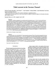
1.2 Ice shelves Ice shelves are the floating extension of the Antarctic Ice Sheet and intimately couple ice sheet and ocean. They are fed by fast flowing ice streams and receive 60% of the continent’s present day accumulation [Giovinetto and Bentley, 1985]. They can range in thickness from 2000 m at the grounding lines where the ice first goes afloat, to 100 m at the ice front and can extend over several hundred kilometres. They comprise 11% of the ice sheet area [Lythe et al., 2000], fringe almost half the Antarctic coast and cover 40% (1.56 x 10⁶ km2) of the Antarctic Continental Shelf (Figure 1.1). Mass loss occurs by both iceberg calving from the seaward margins and melting at the ice shelf base. Uniquely, water masses in the sub-ice shelf cavities are isolated from direct interaction with the atmosphere and the ocean forcing is linked to the exchange of heat, freshwater and momentum at the ice shelf base. The interaction between water masses and ice shelf base result in: regions of strong basal melting particularly near deep grounding lines; the formation of marine ice bodies through the accumulation of ice crystals at the ice shelf base; and the production of seawater at temperatures below the surface freezing point, which have been identified as a component of global bottom water masses [Schlosser et al., 1990; Toggweiler and Samuels, 1995].
1.3 Oceanography of the Southern Ocean The Southern Ocean encircles the entire Antarctic continent and its associated ice shelves, and is bounded by the Antarctic continent to the south and the polar front to the north. This ocean has profound effects on many large scale oceanographic processes, and these effects are evident throughout the world’s oceans. The ocean basins of the Southern Ocean have depths exceeding 4500 m while the relatively deep continental shelves typically have depths
-3-
1.
Introdution 0
Fimbul Ice Shelf
o
Weddell Sea
Filchner Ice Shelf
Amery Ice Shelf
o
o
Ronne Ice Shelf
o
90 W
70 S
80 S
George VI Ice Shelf
o
90 E
Ross Ice Shelf Ross Sea 0
1000
2000
km
Rock and Grounded Ice
180
Ice Shelf
o
Continental Shelf
Deep Ocean
Figure 1.1 Map of Antarctica with surface elevation contours every 500 m reaching a ma ximum e xceeding 4000 m in East Antarctica. The ice shelves (grey) cover 40% of the continental shelf (light blue).
Figure 1.2 Taken from Bearman [1989]. Schematic map showing the circulation in the Southern Ocean. The path of the Antarctic Circumpolar Current (ACC) is shown by the dark blue with the darker lines indicating the average positions of the Antarctic Front and Sub-Antarctic Front. The approximate positions of the gyres in the Weddell Sea and Ross Sea are also shown, as is the path of the Antarctic Coastal Current or Polar Current.
-4-
1.
Introduction
of 300-500 m. Around East Antarctica these shelves are generally narrow (< 200 km) but around West Antarctica they are much broader, and, in the cases of the Weddell and Ross seas, they extend more than 1000 km from the shelf break.
The current structure around the continent is dominated by the Antarctic Circumpolar Current (ACC) that flows in an eastward direction (Figure 1.2) driven by the mean wind stress. Observations show that as the ACC passes through the relatively narrow Drake Passage between South America and the Antarctic Peninsula the transport averages 134 x 106 m3 s-1 [Nowlin and Klinck, 1986]. However, along much of the continental margin there is a narrow westward current, the Antarctic coastal current. This current is not completely circumpolar, but becomes incorporated in the clockwise gyres in the Weddell and Ross seas.
Another feature of the Southern Ocean is the large fluctuations in sea ice extent (Figure 1.3), which varies between 4 x 10⁶ km2 in the austral summer and 21 x 106 km2 in the austral winter when it covers about 60 % of the Southern Ocean. Its formation process is aided by the effect of strong katabatic winds that blow from the continent, forcing the sea ice northward thus forming and maintaining polynyas and allowing further sea ice production over the continental shelf [Bromwich and Kurtz, 1984]. Within these polynyas vigorous cooling and salinisation of surface waters occurs in winter months, particularly in the shore leads around the Antarctic coastline. The process of brine rejection is critical to the ultimate formation of bottom water masses as it densifies surface water masses. These surface water masses decrease the vertical stability of the ocean and enhance mixing via convection down into the water column [e.g. Martinson, 1990; Ushio et al., 1999; Bindoff et al., 2001]. The prevailing offshore movement of the sea-ice creates an export of fresh water ensuring a net brine production in these regions. After modification by shelf break processes or interaction with ice shelves these dense saline waters result in deep and
-5-
1.
a
Introdution
b
September 1979-1999
>96% 92%
84%
76%
February 1979-1999
68%
60%
52%
44%
36%
28%
20%
1500 m). Typically the sub-ice shelf cavity dips downwards towards the grounding line as the seabed deepens and the ice shelf thickens. This geometry has important consequences for the ocean circulation within the cavity.
-11-
W
60°W
C o a s t
70°W
D
R o n n e
D
76°S
I c e
50°W
E
L
30°W
40°W
L
S
E
A
Touchdown Hills
F r o n t
ont
e Fr
r Ic hne
ile
yI
Filc
Hemmen Ice Rise
FILCHNER
O r v i l l e
74°S
E
Ba
74°S
Introduction
R O N N E I C E
ISLAND
Rec o
ver y
S H E L F
ier
lac
rG
sso
Sle
ICE SHELF
BERKNER SITE 2
ce St re am T M he ou ro nt n ai ns
1.
80°S
Shackleton Range
Gla
cier
SITE 1 82°S
SITE 5
Stre
E
ula
SITE 3
e
tr
St
re a
am
m
80°W
tre
e
80°S
78°S
Ic
70°W
82°S
84°S
Pensacola Mountains
eS
Ellsworth Mountains
te
n Ic
eS
atio
Rutfor
c dI
tu
Dufek Massif
am
Fle
sti
m a Skytrain Ice Rise
Stre
e
tch
In
ry
nto
mo
ro rP
Ice
Ca
Inle
ller
n rlso
r lacie
t
F
Mo
Kershaw Ice Rumples
nd
ow
Henry Ice Rise
Fou
P ler
SITE 4
e
ins
en
80°W
Doake Ice Rumples
G rce t Fo por Sup
Ice
Ris f Ice Kor f
s van
ntina Arge nge Ra
am
76°S
50°W
60°W 84°S
40°W
n
Figure 1.6 Map showing Filchner-Ronne Ice Shelf and the flow lines that delineate the discharge from the ten major ice streams that flow into the ice shelf. Geographical locations and drill sites (red dots) cited in the text are also shown.
sio
sula
pr De Ro
nn
o
Ronne Ice front
4
e
S 75
Weddell Sea
es
enin
P rctic Anta
S2 Berkner Shelf
6 6
14
4
S1
6
8
10
er
Fi
n lch
De
ion
ss
e pr
75 o S
12 8
6
Berkner Island 10
12
10
14
14
S5 S4
He
12
16
0
12
10
nry I .R.
14
Korff I .
S3
R.
12
100
200
km
85
S
o
25 o W
o
83
83 o S
W
Figure 1.7 Modified from Nicholls and Makinson [1998]. Map showing the bathymetry in the area of FilchnerRonne Ice Shelf. The contours give bathymetry in 100's of metres below sea level [Johnson and Smith, 1997] and S1, S2, S3, S4 and S5 show the positions of the five drill sites.
-12-
1.
Introduction
1.6 Ice-ocean interactions The Antarctic Ice Sheet annually supplies an average 2.6 x 10¹⁵ kg of freshwater to the Southern Ocean via melting of the ice, either from icebergs or from under ice shelves [Jacobs et al., 1992]. The circulation and associated meltwater input beneath ice shelves have a considerable impact on shelf water masses [e.g. Foldvik et al., 1985b], and up to 75% of the ocean’s deep waters may retain a signature of this meltwater input from beneath FRIS [Toggweiler and Samuels, 1995].
Melting beneath ice shelves relies on seawater having a temperature above the in situ freezing point, which is dependent on the concentration of dissolved salts and the pressure. Both increasing salt content and increasing pressure depresses the freezing point of the seawater. WSW with a salinity of 34.7 psu has a freezing point of -1.9°C. However, it is the depression of the freezing point with pressure that has important implications for ice-ocean interaction, with the freezing point being depressed by 0.00075°C for every decibar increase in pressure. Close to deep grounding lines the freezing point can be up to 1.5°C lower than the surface freezing point, resulting in high melt rates when WSW within the sub-ice shelf cavity comes into contact with the ice shelf base.
Cooling and freshening of seawater caused by melting, forces potential temperature and salinity along a straight line trajectory in 1-S space. For an ice shelf with a temperature profile close to the freezing point, ice/ocean interactions result in water column properties that follow a line with a gradient close to 2.4°C psu-1, whereas for an ice shelf with surface temperatures of -30°C the gradient increases to 2.8°C psu-1 [Gade, 1979]. Because of this relationship, the melt water signature strongly constrains the properties of waters modified beneath ice shelves.
-13-
1.
Introduction
The introduction of glacial melt water into seawater not only modifies its 1-S properties but introduces two tracers important to Antarctic oceanography. Because of the preferential evaporation of 16O over the oceans, snow fall that makes up the glacial ice is low in 18O compared with seawater [Morgan, 1982]. Consequently, glacial melt water is low in 18O, and, by comparing the 18O/16O ratio for inflowing and outflowing water, the concentration of melt water can be calculated, provided the ratio is known for the glacial ice. A second tracer is Helium, which is trapped in air bubbles in the ice and is also released into the water during melting. Because of the low solubility of helium in water, pure glacial meltwater is supersaturated and contains 14 times more Helium than ambient seawater, which has equilibrated with the atmosphere at surface pressure [Schlosser, 1986]. This provides a clear melt water signature, provided that the meltwater-rich outflow has not had the opportunity to re-equilibrate with the atmosphere.
1.7 Sub-ice shelf circulation 1.7.1 Observations The density of the cold water masses found over the continental shelves is determined almost exclusively by salinity. When dense HSSW flows beneath an ice shelf and comes into contact with the ice shelf base it is cooled, but more importantly freshened, leading to buoyant plume of ISW rising up the inclined base of the ice shelf [MacAyeal, 1984b; MacAyeal, 1985a; Jenkins, 1999]. Turbulence within the plume entrains warmer water from below, sustaining melting and maintaining the ISW density below that of the surrounding waters. However, with decreasing depth the freezing point increases and where insufficient heat is entrained, the water becomes supercooled. Under these conditions disc-shaped frazil ice crystals can form and grow, before rising up to be deposited on the ice shelf base and forming marine ice bodies. Robin [1979] suggested that this process could lead to large areas of freezing and using ice-penetrating radar surveys [Robin et al., 1983] mapped the marine ice bodies beneath FRIS (a meteoric ice/ocean interface gives strong radar returns
-14-
1.
Introduction
and meteoric ice/marine ice gives weak returns). Using ice core drilling, Oerter et al., [1992] confirmed the presence of a large marine ice body beneath FRIS. Where marine ice deposits survive to reach the front of ice shelves, calved icebergs that roll over reveal green ice that result from the impurities in the marine ice (Figure 1.8) [Warren et al., 1993]. The water modified beneath the ice shelf by these episodes of melting and freezing ultimately emerges at the ice front as ISW. Within such a core of outflowing ISW on the western side of Filchner Depression, frazil ice platelets of centimetre size have also been observed at a depth of 250 m [Dieckmann et al., 1986].
Most oceanographic work in the southern Weddell Sea has been confined by perennial sea ice to the shore lead along the Filchner-Ronne Ice Front [Foldvik et al., 1985a; Gammelsrød et al., 1994] (Figure 1.9) and in the central part of the Weddell Sea [Gill, 1973; Foster and Carmack, 1976b; Fahrbach et al., 1994]. Ship-borne oceanographic measurements close to the front of ice shelves identify the properties of water masses flowing in and out of the cavity, providing further clues about the sub-ice shelf oceanographic conditions, although they are confined to the short austral summer. However, instrument moorings can also be deployed and, despite the dangers from ice front advance, iceberg calving and the need for
Figure 1.8 An ice berg in the Weddell Sea with bands of green and white marine ice (under sunny conditions). ice [Warren et al., 1993] during its formation from ice crystals that precipitate up from the ocean beneath the ice shelf. (Photo : Keith Makinson).
-15-
1.
Introduction
repeat cruises to recover instruments, a few year-round measurements close to ice fronts have been made [Woodgate et al., 1998; Foldvik et al., 2001].
Observations of the environment beneath Antarctic ice shelves are limited by the presence of the ice shelf itself. Only a small number of direct observations have been made through rifts or access holes drilled through ice shelves, because this usually requires an expensive air-supported operation to transport personnel, equipment and fuel to the drilling sites. Before 1986 there had been no direct observations from beneath FRIS, but using a hot water drill to penetrate the ice shelf, access was gained to the sub-ice shelf cavity [Engelhardt and Determann, 1987]. Using the difference between the depth of the radar reflection and the depth of ice drilled through, Engelhardt and Determann [1987] determined the presence of a 300 m thick layer of marine ice, as well as a 35 m layer of unconsolidated frazil ice at the ice shelf base. Oerter et al., [1992] later obtained a 320 m ice core, about 50 km closer to the ice front, and confirmed the presence of marine ice below a depth of 150 m. Other hot water drilled holes where used to determine basal melt rates and obtain water samples [Grosfeld, 1990]. In the early 1990's groups from the British Antarctic Survey (BAS) and Alfred-Wegener-Institute (AWI) used hot water drills [Makinson, 1993; Nixdorf et al., 1996] to penetrate the ice shelf at several locations on Ronne Ice Shelf. The first sub-ice shelf Conductivity-Temperature-Depth (CTD) profiles were obtained via hot water drilled holes in 1990/91 and 1991/92 [Nicholls et al., 1991; Robinson et al., 1994] and long term thermistor cable moorings to measure temperature were also deployed.
1.7.2 Numerical models Because of the lack of observational data, numerical models have been developed to complement the sparse observations. These range from one-dimensional sub-ice shelf plume models to three-dimensional circulation models that extend out across the
-16-
1.
Introduction
continental shelf and into the deep ocean [Williams et al., 1998]. In turn these models can be used to identify key locations where observational resources should be directed.
Modelling of the thermohaline circulation described above was initially undertaken using one-dimensional plume models that follow the development of the turbulent buoyant plume from grounding line to ice front. The plume of ISW was driven by the density difference between it and the WSW that filled the rest of the cavity. The vertical heat flux required to melt ice and maintain the buoyancy of the plume was obtained by entrainment of the underlying WSW (Figure 1.10). Mixing within the plume resulted from its motion, and the rate of entrainment was determined from the plume velocity and the bulk Richardson number. Where the density contrast fell to zero it was assumed that the plume detached itself from the ice shelf base and exited the cavity at depth (Figure1.10). The first models were applied to Ross Ice Shelf and had some success in simulating the properties of ISW outflows observed at the front of the ice shelf [MacAyeal, 1984b; MacAyeal, 1985a]. Further developments were made by Jenkins [1991] and Nicholls and Jenkins [1993] when a plume model was applied to Ronne Ice Shelf. Good agreement between observed and modelled melt/freeze rates was found along most of the flow line, except near the grounding line and ice front. In these areas tidal effects are likely to be important factors, however these were not included in the model.
More recently, the process of growth and deposition under supercooled conditions of frazil ice crystals, which rise up through the water column and accrete at the ice shelf base has been included in plume models [Bombosch and Jenkins, 1995; Jenkins and Bombosch, 1995]. The frazil ice crystals reduce the bulk density and cause the plume to accelerate, encouraging the growth of more crystals while deposition onto the ice shelf base causes it to decelerate and allow yet more crystals to settle out. As the flow regime usually depends on the basal topography, frazil ice deposition is often intense and highly localized
-17-
1.
Introduction
[Bombosch and Jenkins, 1995]. Bombosch and Jenkins [1995] identified several regions beneath FRIS were their model predicted high basal accumulation rates. These areas agreed reasonably well with the upstream extremity of the marine ice bodies beneath the ice shelf.
A two-dimensional circulation model has been used to attempt to calculate the likely circulations beneath FRIS [Hellmer and Olbers, 1989; Hellmer and Olbers, 1991]. The circulation was assumed to follow the ice thickness gradient and, as with the plume models, lateral variations in ice shelf gradients and the effects of Coriolis and tides were ignored. The circulation pattern between the interconnected cavities of Filchner Ice Shelf and Ronne Ice Shelf were examined using three differing geometries. In all cases each cavity was dominated by a single overturning cell with regions of melting and freezing. Two of the geometries used a shallow water column at the front of Ronne Ice Shelf. In these cases outflowing ISW occupied the whole water column at Ronne Ice Front, so both cavities were supplied with WSW from the inflow at Filchner Ice Front. Within the cavity beneath Ronne Ice Shelf the model indicated that water may recirculate several times before leaving the cavity as ISW. For the third geometry, a thicker water column at Ronne Ice Front allowed WSW to inflow. A stronger circulation developed beneath Ronne Ice Shelf because of the large density gradients between the inflow and outflow. Some of the inflow from Ronne Ice Front also supported the weaker circulation beneath Filchner Ice Shelf.
Determann and Gerdes [1994] applied the first three-dimensional circulation model to the sub-ice shelf domain. It incorporated the effects of the Earth’s rotation on the ocean dynamics which had been neglected in previous sub-ice shelf modelling efforts. The model results highlighted that the circulation was constrained to follow the f/H contours, where f is the Coriolis parameter and H is the water column depth. The ice front consequently presented a considerable barrier to water mass exchange between the cavity and open ocean. Also, internal recirculation was indicated with regions of intense melting and
-18-
1.
Submarine Ridge
Berkner Shelf
Filchner Depression -1.0
-1.6 -1.9 -1.8
-1.6 -1.9
-1.8
-1.6 -1.4
-1.8
-2.0
-2.0
0
-1.95
-1.95
-2.
-200
-1.9
-1.8 -1.9
400
0
Berkner Island
0 30
Ronne Depression
Introduction
-1.9
-2.0 -2.1 -2.2
-400 -600
-2.1 -1.95 -2 .0
-2.1
-800 -1.95
-1000 -1200 o
o
o
o
o
o
60 W
55 W
50 W
45 W
40 W
35 W
Figure 1.9 Section of potential temperature along the ice front fromRonne depression to the Filchner Depression [after Foldvik et al., 1985c]. ISW colder than -2.0°C is shown in blue and MWDW above -1.6°C is shown in red. The bathymetry is represented by the dark shading.
Open shore lead
Wind
Northward transport of sea ice
o
Convection
Ice Shelf ei
MW
ce
zin ee
En
tr
m
t
t Con
ine
nt
WSW f hel al S
Me
ltin
g
Fr
en n ai
WW DW
ISW
g
M
n ari
ISW
Pressure freezing point of seawater
-1.9 C
WDW
-3.0oC
Bedrock
WSBW
Figure 1.10 Schematic of the circulation over the continental shelf and beneath Filchner-Ronne Ice Shelf. At the continental shelf break Weddell Deep Water (WDW) mixes with Winter Water (WW) to form Modified Weddell Deep Water (MWDW) that intrudes across the continental shelf. Close to the ice front, Western Shelf Water (WSW) is formed by salt release during sea ice formation, particularly in the shore lead which is maintained through the winter by offshore winds and tidal currents. Where the WSW comes into contact with the ice shelf base at depth melting takes place due to the depression of the freezing point. This process forms buoyant Ice Shelf Water (ISW) which rises up the ice shelf base, further melting takes place until the ISW becomes super cooled and freezing takes place. The ISW exits the cavity at depth, crossing the continental shelf before descending the continental slope to form Weddell Sea Bottom Water (WSBW) and ultimately Antarctic Bottom Water (AABW).
-19-
1.
Introduction
freezing driving the flow. Extending the model to include the open ocean and atmospheric forcing, Grosfeld et al. [1997] found that the slopes of the Ronne and Filchner depressions were important. Here, the f/H contours cross the ice front with only a small lateral displacement, thus allowing the flow to cross the ice front, while elsewhere the ice front remained a barrier (Figure 1.11).
A drawback with all the sub-ice shelf thermohaline models outlined above is that they do not consider the impact of tidal forcing. In an environment isolated from atmospheric forcing, oscillatory tidal currents can generate residual circulations and provide a significant source of turbulent kinetic energy. These processes may be important to ice front exchanges and the vertical heat flux through the water column, both of which might lead to modification of the sub-ice shelf thermohaline circulation.
0
Depth (m)
-200
b
Ice Shelf
0 -200
-400
-400
-600
-600
-800
-800
Depth (m)
a
-1000 -1200
Bedrock
-1400
-1000 -1200
-1600
-1800
-1800
o
78 S
o
76 S
Bedrock
-1400
-1600
-2000 o 80 S
Ice Shelf
o
74 S
o
72 S
o
70 S
o
68 S
-2000 80oS
78oS
76oS
74oS
72oS
70oS
68oS
Latitude
Latitude
Figure 1.11 Taken from Grosfeld et al. [1997]. Stream function of the zonally integrated mass transport for two versions of thethree-dimensional model using idealised geometry patterned on that found in the southern Weddell Sea. (a) Contains an ice shelf cavity, open continental shelf and open deep ocean. The contour interval beneath the ice shelf is 0.01 Sv and 0.05 Sv in the open ocean. (b) Same as (a) but two 900 m deep depressions cross either side of the continental shelf. The contour interval 0.05 Sv (1 Sv = 10 6 m3 s-1).
-20-
1.
Introduction
1.8 Ocean tides Tidal energy is propagated from astronomical forcing of the oceans to the continental shelves, and is eventually dissipated by bottom friction in shallow water through the generation of turbulence. The most recent estimates of the rate of global energy input into the worlds ocean from astronomical forcing determined from satellite observations is 2.4 TW, with estimates through analysis of orbit perturbations, satellite altimetry and hydrodynamic models yielding similar dissipation rates [Le Provost and Lyard, 1997; Munk, 1997]. Isolated from direct atmospheric forcing, tides may represent the most energetic currents within a sub-ice shelf cavity.
The presence of an ice shelf provides a solid boundary at the top of the water column with effectively no horizontal motions, so its dynamical influence is to exert drag on the motion of the water, much like that exerted by the seabed. For vertical motions the ice shelf can be considered a free surface with no flexural rigidity, so it rises and falls passively with the tides. Only within a few kilometres of the grounding lines is this a poor assumption [MacAyeal, 1984a; Vaughan, 1995]. The draft of the ice shelf effectively reduces the water column thickness, with a step change in water column thickness occurring at the ice front.
Tides play a role in the atmosphere-ice-ocean system. Tidal currents help maintain shore leads along the front of ice shelves [Foldvik and Gammelsrød, 1988] and divergence in the current field maintains further leads, particularly near the continental shelf break [Padman and Kottmeier, 2000]. The generation of mean tidal currents or residual currents through the interaction of tidal oscillations with topography will advect water masses, particularly along ice fronts [MacAyeal, 1985b]. Vertical mixing can help modify water masses through turbulent mixing at the seabed and ice shelf base, and beneath ice shelves vertical mixing can enhance basal melting.
-21-
1.
Introduction
In the seas around the Antarctic continent the largest observed tidal range is in the southwest corner of Ronne Ice Shelf. Near the grounding line of Rutford Ice Stream a gravimeter record, dominated by semi-diurnal tides, showed peak-to-peak displacements of about 6 m [Doake, 1992]. Recently, Padman et al. [2002] used a circum-Antarctic tidal model to confirm that the largest tides occur in the Southern Weddell Sea and that in the channel south of Henry and Korff ice rises the tidal range can exceed 7 m during spring tides. In the Ross Sea, which is dominated by diurnal tides, the range does not exceed 2 m except close to the southern Siple Coast [Padman et al., 2002].
Tidal models that include the cavity beneath FRIS within their domains such as Genco et al. [1994] and Smithson et al. [1996] have only investigated tidal elevations. Beneath Ross Ice Shelf it has been suggested that tidal currents and their associated mixing maybe one of the primary controls on the strength of the thermohaline circulation and that tidal rectification may help drive water masses in and out of the cavity [MacAyeal, 1984b; MacAyeal, 1985b]. Scheduikat and Olbers [1990] made a more detailed study of tidally induced vertical mixing and its effect on melting and freezing at the ice-ocean interface beneath Ross Ice Shelf with moderate success. When compared with Ross Ice Shelf, FRIS has greater levels of tidal activity. Clearly, to understand how the sub-ice shelf system works in detail, tidal activity beneath FRIS needs to be considered [Williams et al., 1998].
-22-
1.
Introduction
1.9 References Bearman, G., Ocean Circulation, Open University and Pergamon Press, 1989. Bindoff, N.L., G.D. Williams, and I. Allison, Sea-ice growth and water-mass modification in the Mertz Glacier polynya, East Antarctica, during winter, in Annals of Glaciology, Vol 33, pp. 399-406, 2001. Bombosch, A., and A. Jenkins, Modeling the Formation and Deposition of Frazil Ice beneath Filchner-Ronne Ice Shelf, Journal of Geophysical Research, 100 (C4), 6983-6992, 1995. Broecker, W.S., S.L. Peacock, S. Walker, R. Weiss, E. Fahrbach, M. Schroeder, U. Mikolajewicz, C. Heinze, R. Key, T.H. Peng, and S. Rubin, How much deep water is formed in the Southern Ocean?, Journal of Geophysical Research-Oceans, 103 (C8), 15833-15843, 1998. Bromwich, D.H., and D.D. Kurtz, Katabatic Wind Forcing of the Terra-Nova Bay Polynya, Journal of Geophysical Research-Oceans, 89 (C3), 3561-3572, 1984. Determann, J., and R. Gerdes, Melting and freezing beneath ice shelves: implications from a threedimensional ocean-circulation model, Annals of Glaciology, 20, 413-419, 1994. Dieckmann, G., G. Rohardt, H. Hellmer, and J. Kipfstuhl, The occurrence of ice platelets at 250 m depth near the Filchner Ice Shelf and its significance for sea ice biology, Deep-Sea Research, 33 (2), 141-148, 1986. Doake, C.S.M., Gravimetric tidal measurements on Filchner-Ronne Ice Shelf, in Filchner Ronne Ice Shelf Programme Report, pp. 34-39, Alfred-Wegener-Institute, Bremerhaven, Germany, 1992. Engelhardt, H., and J. Determann, Borehole Evidence for a Thick Layer of Basal Ice in the Central Ronne Ice Shelf, Nature, 327 (6120), 318-319, 1987. Fahrbach, E., S. Harms, G. Rohardt, M. Schröder, and R.A. Woodgate, Flow of bottom water in the northwestern Weddell Sea, Journal of Geophysical Research-Oceans, 106 (C2), 2761-2778, 2001. Fahrbach, E., G. Rohardt, N. Scheele, M. Schröder, V. Strass, and A. Wisotzki, Formation and Discharge of Deep and Bottom Water in the Northwestern Weddell Sea, Journal of Marine Research, 53 (4), 515538, 1995. Fahrbach, E., G. Rohardt, M. Schröder, and V. Strass, Transport and structure of the Weddell Gyre, Annales Geophysicae, 12, 840-855, 1994. Foldvik, A., and T. Gammelsrød, Notes on Southern Ocean hydrography, sea-ice and bottom water formation, Palaeogeography, Palaeoclimatology, Palaeoecology, 67, 3-17, 1988. Foldvik, A., T. Gammelsrød, E. Nygaard, and S. Østerhus, Current meter measurements near Ronne Ice Shelf, Weddell Sea: Implications for circulation and melting underneath the Filchner-Ronne ice shelves, Journal of Geophysical Research, 2001. Foldvik, A., T. Gammelsrød, N. Slotsvik, and T. Tørresen, Oceanographic conditions on the Weddell Sea Shelf during the German Antarctic Expedition 1979/80, Polar Research, 3 (2), 209-226, 1985a. Foldvik, A., T. Gammelsrød, and T. Tørresen, Circulation and water masses on the Southern Weddell Sea Shelf, in Oceanology of the Antarctic Continental Shelf, edited by S.S. Jacobs, pp. 5-20, American Geophysical Union, Washington DC, 1985b. Foldvik, A., T. Gammelsrød, and T. Tørresen, Hydrographic observations from the Weddell Sea during the Norwegian Antarctic Research Expedition 1976/77, Polar Research, 3 (2), 177-193, 1985c. Foldvik, A., T. Gammelsrød, and T. Tørresen, Physical oceanography studies in the Weddell Sea during the Norwegian Antarctic Research Expedition 1978/79, Polar Research, 3 (2), 195-207, 1985d. Foster, T.D., and E.C. Carmack, Frontal zone mixing and Antarctic Bottom Water formation in the southern Weddell Sea, Deep-Sea Research, 23, 301-317, 1976a. Foster, T.D., and E.C. Carmack, Temperature and salinity structure in the Weddell Sea, Journal of Physical Oceanography, 6, 36-44, 1976b. Foster, T.D., A. Foldvik, and J.H. Middleton, Mixing and Bottom Water Formation in the Shelf Break Region of the Southern Weddell Sea, Deep-Sea Research Part a-Oceanographic Research Papers, 34 (11), 1771-1794, 1987.
-23-
1.
Introduction
Fox, A.J., and A.P.R. Cooper, Measured properties of the Antarctic ice sheet derived from the SCAR Antarctic digital database, Polar Record, 30, 201-206, 1994. Gade, H.G., Melting of Ice in Sea Water: A Primitive Model with Application to the Antarctic Ice Shelf and Icebergs, Journal of Physical Oceanography, 9 (1), 189-198, 1979. Gammelsrød, T., A. Foldvik, O.A. Nøst, Ø. Skagseth, L.G. Anderson, E. Fogelqvist, K. Olsson, T. Tanhua, E.P. Jones, and S. Østerhus, Distribution of water masses on the continental shelf in the Southern Weddell Sea, in The polar oceans and their role in shaping the global environment, edited by O.M. Johannesen, R.D. Muench, and J.E. Overland, pp. 159-176, AGU, Washington DC, 1994. Ganachaud, A., and C. Wunsch, Improved estimates of global ocean circulation, heat transport and mixing from hydrographic data, Nature, 408 (6811), 453-457, 2000. Genco, M.L., F. Lyard, and C. Le Provost, The Oceanic Tides in the South-Atlantic Ocean, Annales Geophysicae, 12 (9), 868-886, 1994. Gill, A.E., Circulation and bottom water production in the Weddell Sea, Deep-Sea Research, 20, 111-140, 1973. Giovinetto, M.B., and C.R. Bentley, Surface balance in ice drainage systems in Antarctica, Antarctic Journal of the US, 20 (4), 6-13, 1985. Gordon, A.L., B.A. Huber, H.H. Hellmer, and A. Ffield, Deep and Bottom Water of the Weddell Seas Western Rim, Science, 262 (5130), 95-97, 1993. Grosfeld, K., Temperature profiles and investigation of the ice-shelf/ocean boundary using hot water drilled holes: report of field work on FRIS 1989/90, in Filchner Ronne Ice Shelf Programme Report No 4, edited by H. Oerter, pp. 109-111, Alfred-Wegener-Institute for Polar and Marine Research, Bremerhaven, Germany, 1990. Grosfeld, K., N. Blindow, and F. Thyssen, Bottom melting on the Filchner-Ronne Ice Shelf, Antarctica, using different measuring techniques, Polarforschung, 62, 71-76, 1992. Grosfeld, K., R. Gerdes, and J. Determann, Thermohaline circulation and interaction between ice shelf cavities and the adjacent open ocean, Journal of Geophysical Research, 102 (C7), 15595-15610, 1997. Hellmer, H.H., and D.J. Olbers, A two-dimensional model for the thermohaline circulation under an ice shelf, Antarctic Science, 1, 325-336, 1989. Hellmer, H.H., and D.J. Olbers, On the Thermohaline Circulation beneath the Filchner-Ronne Ice Shelves, Antarctic Science, 3 (4), 433-442, 1991. Jacobs, S.S., R.G. Fairbanks, and Y. Horibe, Origin and evolution of water masses near the Antarctic Continental Margin: Evidence from H218O/H216O ratios in seawater, in Oceanology of the Antarctic Continental Shelf, edited by S.S. Jacobs, pp. 59-85, American Geophysical Union, Washington DC, 1985. Jacobs, S.S., H.H. Helmer, C.S.M. Doake, A. Jenkins, and R.M. Frolich, Melting of Ice Shelves and the Mass Balance of Antarctica, Journal of Glaciology, 38 (130), 375-387, 1992. Jenkins, A., A One-Dimensional Model of Ice Shelf-Ocean Interaction, Journal of Geophysical Research, 96 (C11), 20671-20677, 1991. Jenkins, A., The impact of melting ice on ocean waters, Journal of Physical Oceanography, 29 (9), 23702381, 1999. Jenkins, A., and A. Bombosch, Modeling the Effects of Frazil Ice Crystals on the Dynamics and Thermodynamics of Ice Shelf Water Plumes, Journal of Geophysical Research, 100 (C4), 69676981, 1995. Johnson, M.R., and A.M. Smith, Seabed topography under the southern and western Ronne Ice Shelf, derived from seismic surveys, Antarctic Science, 9 (2), 201-208, 1997. Killworth, P.D., Mixing in the Weddell Sea continental slope, Deep Sea Res, 24, 427-448, 1977.
-24-
1.
Introduction
Le Provost, C., and F. Lyard, Energetics of the M-2 barotropic ocean tides: an estimate of bottom friction dissipation from a hydrodynamic model, Progress in Oceanography, 40 (1-4), 37-52, 1997. Lythe, M.B., D.G. Vaughan, and the BEDMAP consortium, BEDMAP - bed topography of the Antarctic, 1:10 000 000 scale map., British Antarctic Survey, Cambridge, 2000. MacAyeal, D.R., Numerical Simulations of the Ross Sea Tides, Journal of Geophysical Research, 89 (C1), 607-615, 1984a. MacAyeal, D.R., Thermohaline Circulation Below the Ross Ice Shelf - a Consequence of Tidally Induced Vertical Mixing and Basal Melting, Journal of Geophysical Research, 89 (C1), 597-606, 1984b. MacAyeal, D.R., Evolution of tidally triggered meltwater plumes below ice shelves, in Oceanology of the Antarctic Continental Shelf, edited by S.S. Jacobs, pp. 133-143, American Geophysical Union, Washington DC, 1985a. MacAyeal, D.R., Tidal rectification below the Ross Ice Shelf, Antarctica, in Oceanology of the Antarctic Continental Shelf, edited by S.S. Jacobs, pp. 109-132, American Geophysical Union, Washington DC, 1985b. Makinson, K., The Bas Hot-Water Drill - Development and Current Design, Cold Regions Science and Technology, 22 (1), 121-132, 1993. Makinson, K., Modeling tidal current profiles and vertical mixing beneath Filchner-Ronne Ice Shelf, Antarctica, Journal of Physical Oceanography, 32(1), 202-215, 2002. Makinson, K., and K.W. Nicholls, Modeling tidal currents beneath Filchner-Ronne Ice Shelf and on the adjacent continental shelf: their effect on mixing and transport, Journal of Geophysical Research, 104 (C6), 13449-13465, 1999. Mantyla, A.W., and J.L. Reid, Abyssal Characteristics of the World Ocean Waters, Deep-Sea Research Part A-Oceanographic Research Papers, 30 (8), 805-&, 1983. Martinson, D.G., Evolution of the Southern-Ocean Winter Mixed Layer and Sea Ice - Open Ocean DeepWater Formation and Ventilation, Journal of Geophysical Research-Oceans, 95 (C7), 11641-11654, 1990. Meredith, M.P., A.J. Watson, and K.A. Van Scoy, Chlorofluorocarbon-derived formation rates of the deep and bottom waters of the Weddell Sea, Journal of Geophysical Research-Oceans, 106 (C2), 28992919, 2001. Morgan, V.I., Antarctic Ice-Sheet Surface Oxygen Isotope Values, Journal of Glaciology, 28 (99), 315-323, 1982. Muench, R.D., and A.L. Gordon, Circulation and Transport of Water Along the Western Weddell Sea Margin, Journal of Geophysical Research-Oceans, 100 (C9), 18503-18515, 1995. Munk, W., Once again: Once again - tidal friction, Progress in Oceanography, 40 (1-4), 7-35, 1997. Nicholls, K.W., and A. Jenkins, Temperature and Salinity beneath Ronne Ice Shelf, Antarctica, Journal of Geophysical Research, 98 (C12), 22553-22568, 1993. Nicholls, K.W., and K. Makinson, Ocean circulation beneath the western Ronne Ice Shelf, as derived from in situ measurements of water currents and properties, in Ocean, Ice, and Atmosphere: Interactions at the Antarctic Continental Margin, edited by S.S. Jacobs, and R.F. Weiss, pp. 301-318, American Geophysical Union, Washingtion DC, 1998. Nicholls, K.W., K. Makinson, and A.V. Robinson, Direct oceanographic observations from under the Rutford flowline, Ronne Ice Shelf., in Filchner Ronne Ice Shelf Programme Report No 5, edited by H. Oerter, pp. 27-31, Alfred-Wegener-Institute for Polar and Marine Research, Bremerhaven, Germany, 1991. Nixdorf, U., H. Oerter, and H. Miller, The Hot-Water Drilling System of the Alfred Wegener Institute fur Polar und Meeresforschung (AWI), in Proceedings of the 7th SCALOP symposium on Antarctic logistics and operations, pp. 203, Cambridge, UK, 1996.
-25-
1.
Introduction
Nowlin, W.D., and J.M. Klinck, The Physics of the Antarctic Circumpolar Current, Reviews of Geophysics, 24 (3), 469-491, 1986. Oerter, H., J. Kipfstuhl, J. Determann, H. Miller, D. Wagenbach, A. Minikin, and W. Graf, Evidence for Basal Marine Ice in the Filchner-Ronne Ice Shelf, Nature, 358 (6385), 399-401, 1992. Padman, L., H.a. Fricker, R. Coleman, S. Howard, and L. Erofeeva, A New Tidal Model for the Antarctic Ice Shelves and Seas, Annals of Glaciology, In Press, 2002. Padman, L., and C. Kottmeier, High-frequency ice motion and divergence in the Weddell Sea, Journal of Geophysical Research, 105 (C2), 3379-3400, 2000. Robin, G.D., C.S.M. Doake, H. Kohnen, R.D. Crabtree, S.R. Jordan, and D. Moller, Regime of the FilchnerRonne Ice Shelves, Antarctica, Nature, 302 (5909), 582-586, 1983. Robin, G.d.Q., Formation, flow, and disintegration of ice shelves, Journal of Glaciology, 24, 259-271, 1979. Robinson, A., K. Makinson, and K. Nicholls, The oceanic environment beneath the north-west Ronne Ice Shelf, Antarctica, Annals of Glaciology, 20, 386-390, 1994. Scheduikat, M., and D.J. Olbers, A one-dimensional mixed layer model beneath the Ross Ice Shelf with tidally induced vertical mixing, Antarctic Science, 2, 29-42, 1990. Schlosser, P., Helium: a new tracer in Antarctic oceanography, Nature, 321, 233-235, 1986. Schlosser, P., R. Bayer, A. Foldvik, T. Gammelsrød, G. Rohardt, and K.O. Munnich, O-18 and Helium as Tracers of Ice Shelf Water and Water Ice Interaction in the Weddel Sea, Journal of Geophysical Research, 95 (C3), 3253-3263, 1990. Smithson, M.J., A.V. Robinson, and R.A. Flather, Ocean tides under the Filchner-Ronne Ice Shelf, Antarctica, Annals of Glaciology, 23, 217-225, 1996. Toggweiler, J.R., and B. Samuels, Effect of Sea-Ice on the Salinity of Antarctic Bottom Waters, Journal of Physical Oceanography, 25 (9), 1980-1997, 1995. Ushio, S., T. Takizawa, K.I. Ohshima, and T. Kawamura, Ice production and deep-water entrainment in shelf break polynya off Enderby Land, Antarctica, Journal of Geophysical Research-Oceans, 104 (C12), 29771-29780, 1999. Vaughan, D.G., Tidal Flexure at Ice Shell Margins, Journal of Geophysical Research, 100 (B4), 6213-6224, 1995. Warren, S.G., C.S. Roesler, V.I. Morgan, R.E. Brandt, I.D. Goodwin, and I. Allison, Green icebergs formed by freezing of organic-rich seawater to the base of Antarctic ice shelves, Journal of Geophysical Research, 98, 6921-6928, 1993. Weppernig, R., P. Schlosser, S. Khatiwala, and R.G. Fairbanks, Isotope data from Ice Station Weddell: Implications for deep water formation in the Weddell Sea, Journal of Geophysical Research-Oceans, 101 (C11), 25723-25739, 1996. Williams, M.J.M., A. Jenkins, and J. Determann, Physical controls on ocean circulation beneath ice shelves revealed by numerical models, in Ocean, Ice, and Atmosphere: Interactions at the Antarctic Continental Margin, edited by S.S. Jacobs, and R. Weiss, pp. 285-299, AGU, Washington DC, 1998. Woodgate, R.A., M. Schrøder, and S. Østerhus, Moorings from the Filchner Trough and the Ronne Ice Shelf Front: Preliminary Results, in Filchner Ronne Ice Shelf Programme Report No 12, edited by H. Oerter, pp. 85-90, Alfred-Wegener-Institute for Polar and Marine Research, Bremerhaven, Germany, 1998.
-26-
2.
Field Work on Filchner-Ronne Ice Shelf
CHAPTER 2 Field Work on Filchner-Ronne Ice Shelf 2.1 Introduction 2.1.1 History of sub-ice shelf oceanography Prior to direct observations, sub-ice shelf circulation has generally been inferred from ship-borne ice front measurements [e.g. Foldvik et al., 1985; Nøst and Foldvik, 1994; Nøst and Østerhus, 1998]. Direct oceanographic observations beneath ice shelves are limited by the presence of the ice shelf itself, which varies in thickness from a few hundred metres to 2 km. Furthermore, the remoteness of the sites selected for direct observations require an expensive logistical operation to transport personnel, equipment and fuel to field locations using ski-equipped aircraft. At present the only way of gaining direct oceanographic measurements from beneath ice shelves is by drilling access holes and using oceanographic instruments modified for borehole deployment.
In 1977, as part of the Ross Ice Shelf Project, an access hole was drilled using a flame-jet drill through 420 m of ice at Site J-9 (82°22.5'S 168°37.5'W) [Clough and Hansen, 1979] allowing oceanographic profiles of the 240 m thick water column to be obtained over a six-day period [Foster, 1983]. Such access holes to the underlying seawater allow CTD profiles of the water column to be obtained together with water samples that can be analysed for oceanographic tracers such as *18O and *D. The salinity, temperature and tracers collectively provide a "signature" of the water masses that can be used to identify the origins of the water and their subsequent interactions with the ice shelf. Once oceanographic profiling has been completed, it is possible to deploy a range of
-27-
2.
Field Work on Filchner-Ronne Ice Shelf
instrumentation to monitor temperature, conductivity, and current speed and direction. These instruments can be regularly logged to provide long term measurements from within the ice shelf, the water column and across the ice/ocean interface. Such data sets can reveal changes in ice shelf temperatures [Paren and Cooper, 1988], basal melt rates [Grosfeld and Blindow, 1993] and fluctuations in the characteristics of the water column [Nicholls et al., 1991]. Knowledge of these directly observed parameters beneath ice shelves aids mass balance studies, the understanding of the dynamics of ice shelf and ocean, and the ice/ocean interaction. Besides Ross Ice Shelf, a small number of CTD observations have also been made beneath George VI Ice Shelf [Cooper et al., 1988], Fimbul Ice Shelf [Østerhus and Orheim, 1992], Ronne Ice Shelf [Nicholls and Makinson, 1998; Nicholls et al., 2001] and most recently Amery Ice Shelf [Mike Craven, Pers. com., 2001].
On FRIS the first CTD profiles from beneath the ice shelf were obtained in January 1991. A hot water drill was used to penetrate ice 562 m thick at Site 1 about 300 km from the ice front in the western area of Ronne Ice shelf (Figure 2.1). A borehole deployable CTD and water sampling system was used to obtain the first in situ information from the 364-m deep water column [Nicholls et al., 1991]. In the following year, an access hole at Site 2 yielded more in situ data from the eastern flank of Ronne Depression [Robinson et al., 1994; Robinson and Makinson, 1994], 200 km from the ice front. Here ice 541 m thick overlies a 400 m water column. At both these sites, CTD sections and water samples were obtained and long term thermistor cables deployed with data initially transmitted via satellite link. Site 3 was occupied in January 1996 and was located 500 km from the ice front and 17 km west of Korff Ice Rise where 825 m of ice overlies a 485-m deep water column [Nicholls et al., 1997]. CTD sections and water samples were obtained. An oceanographic mooring was deployed for long term measurements that consisted of two current meters and five Conductivity-Temperature-Pressure (CTP) units. A thermistor cable was also deployed that extended down to the first current meter, about 20 m below the ice base. All data were
-28-
2.
Field Work on Filchner-Ronne Ice Shelf
recorded locally in a data logger with data from mooring also being transmitted via satellite link.
2.1.2 Aims of fieldwork The aim of the field work was to acquire further unique oceanographic data in the ocean cavity beneath FRIS that could address some of the unresolved oceanographic questions. The work described here is a continuation of an investigation into the oceanographic regime beneath FRIS that began in the early 1990's. The focus is away from the western Ronne Ice Shelf of sites 1, 2 and 3, to the south eastern corner of Ronne Ice Shelf and westernmost Filchner Ice Shelf. The aim was to provide data on water column structure and circulation, estimated rates of melting and/or freezing, water mass residence times and source locations as well as seasonal variations, tidal currents and vertical energy fluxes. These data will be used to validate the tidal model in Chapter 4, evaluate residual tidal currents in Chapter 5 and the contribution of tides to the vertical heat flux in Chapter 7. The data sets will also be used by others to help control the large scale circulation models that are applied to the sub-ice shelf cavity. The remainder of this chapter describes the techniques and instruments employed in gathering sub-ice shelf oceanographic data.
2.2 Gaining access - Hot water drilling 1998/99 2.2.1 Logistical constrains and site locations Both Antarctica itself and the BAS logistics infrastructure place limitations on the hot water drilling/oceanographic work. The use of Twin Otter aircraft to establish field camps limits the maximum size of single items of equipment such as drill winches, oceanographic moorings and snowmobiles (skidoos), with some items having to be broken down and reassembled in the field. Each item must also be light enough to be hand-manageable by four or fewer personnel, working on soft snow. With Twin Otter payloads of around 2000 lbs, deployment of equipment, fuel and personnel requires many input flights. The -29-
2.
Field Work on Filchner-Ronne Ice Shelf
South America
50°
60°
Port Stanley Falkland Islands
70°W
40°
Bird Island
sage
Pas rake
D
Signy
60°
en
s au h s ing Sea l l e
We dd ell Se a
Rothera
B
Fossil Bluff
George VI Ice Shelf Sky-Hi 70
°
Site 2
Halley
Site 1
Touchdown Hills
Site 3 Site 5
Fimbul Ice Shelf
Site 4
S 0°
Filchner Ice Shelf
Ronne Ice Shelf
8
500
0
500
1000
kilometres
Figure 2.1 Location map showing the logistical routes (red) to the drill sites on Filchner-Ronne Ice Shelf via various permanent stations and field fuel depots using both ships and aircraft. The ice shelves are shaded in grey.
-30-
2.
Field Work on Filchner-Ronne Ice Shelf
large distance to the nearest station requires the aircraft to refuel at least once or twice, therefore the flying hours required to service both the fuel depots and the field site increase rapidly with distance from a station. Consequently, the number of instrumented sites across FRIS is limited because of the expense of this type of work. Sites are chosen on the basis of testing as many sub-ice shelf circulation models as possible, the aim being to disprove models as clearly as possible. Ideally, the observational data should identify the model(s) that most closely match the physical processes occurring beneath FRIS, rather than provide only partial agreement for several models.
Previous hot water drilling work on Ronne Ice Shelf (sites 1, 2 and 3) has been supported from Rothera Station using Twin Otter aircraft. The aircraft refuel at permanent fuel depots at Fossil Bluff on the east coast of Alexander Island, and at Sky-Hi in the Sweeney Mountains, southern Palmer Land (Figure 2.1). These depots are also supported from Rothera Station. After the completion of drilling at Site 3, a depot of drilling equipment was established at Site 4 (80°59.1' S 51°36.4' W) in January 1996 between Berkner Island and the Dufek Coast, 12 km south of Berkner Island. Fuel depots were placed at both Site 4 and Site 5 (80°20.0' S 54°46.4) in the following years, with Site 5 located between Berkner Island and Henry Ice Rise, 17 km west of the southwestern coast of Berkner Island. The 1998/99 fieldwork at sites 4 and 5 was primarily supported from Halley Station on the Brunt Ice Shelf because of its proximity, only 800 km distant, as opposed to Rothera Station, more than 1500 km to the north. The remaining drilling and oceanographic equipment was in place by the end of December 1998, having been flown by Twin Otter from Halley Station via a fuel depot at Touchdown Hills (Figure 2.1)
2.2.2 Local seismic surveys Bathymetric and ice thickness data had previously been obtained in the vicinity of Site 4 [Johnson and Smith, 1997] and were used to identify the best location for the drill site. In
-31-
00
SITE 4
-12 . . . . . . . .
c
0 -14 . . .
.
.
.
0 .
.
.
. . . . 0 - 1. 4 0 . . . . . .
. . . . . . . . . . . . .
. . . . . . .
0 -14 .
.
.
0
.
.
.
. . .
.
Berkner I.
d
. . . . 0 - 1. 4 0 . . . . . .
Dufek
Berkner I.
Henry IR 0
0 SITE 4
Ice shelf
0.4
Depth (km)
Depth (km)
SITE 5
Dufek
Dufek
0.8
SITE 5
Ice shelf
0.4 0.8 1.2
1.2 1.6
Berkner Island
Henry I. R.
Henry I. R. . . . . . . . . . . . . .
b
Berkner Island
00
a
Field Work on Filchner-Ronne Ice Shelf
-12
2.
1.6
Bedrock 0
20
40 60 80 Distance (km)
100
e
40
60 80 Distance (km)
100
120
600
650
N
Site 4
85 0
20
f
82 5
N
Bedrock 0
120
Site 5
70 0
87 5 90 0
0
km
g
h
1450 1500
110 0
N
km
20
700 800 900 0 100
N
0
20
Site 4
Site 5 12 00
1450 1400
1300
0
km
20
0
km
20
Figure 2.2 Modified from Nicholls et al. [2001]. Topography in the vicinity of sites 4 and 5, as determined by local seismic surveys. The areas covered by the survey are indicated by the highlighted boxes in (a) and (b) together with the path of the cross sections shown in (c) and (d). The cross sections show the thickness of ice shelf and water column with the vertical dashed lines indicating the location of the drill sites. Markers on the ice and bedrock surfaces indicate the location of seismic stations along the section. Contours of ice shelf draft in metres around Sites 4 and 5 are shown in (e) and (f) with the dots showing the locations of seismic measurements The shaded area is grounded ice (the coast) and the arrows indicate the velocity of the mean flow. (g) and (h) show the contours of bedrock depth from the local survey around the drill sites.
-32-
2.
Field Work on Filchner-Ronne Ice Shelf
the vicinity of Site 5, previously existing bathymetric maps [Vaughan et al., 1994] were based on only a few scattered data points. Local seismic surveys were performed by a two-man travelling party (Mark Johnson and Steve Hinde) around each of the drill sites at a grid spacing of 5 to 10 km to both refine the selection of the drill sites and to aid in the interpretation of the data [Nicholls et al., 2001]. Maps showing contours of ice shelf draft and bedrock topography are given in Figure 2.2 together with cross sections running out from the coast of Berkner Island to the Dufek Massif coast and Henry Ice Rise. Both bedrock and ice base topography are smooth at this resolution with the Site 4 section showing a mid-channel ridge, flat ice base and steep slope towards the Berkner Island Coast. The Site 5 section shows a relatively gentle rise in the bedrock towards the Berkner Island coast that is accompanied by a similar rise in the ice base.
2.2.3 Drilling system description The BAS hot water drill was initially developed to obtain direct oceanographic observations from beneath George VI Ice Shelf and more recently Ronne Ice Shelf. The original Hot Water Drill (HWD) provided a means of rapidly gaining access to the sea water beneath George VI Ice Shelf for a period of hours or days [Cooper et al., 1988]. Through the 1990's the work on Ronne Ice Shelf placed more demands on the HWD, and I adapted ideas from other drilling projects such as the Ross Ice Shelf Project at J-9, Antarctica [Koci, 1984], Jakobshavns Glacier, Greenland [Iken et al., 1989], Ice Stream B, Antarctica [Humphrey and Echelmeyer, 1990]. I successfully incorporated these ideas into the BAS hot water drilling system [Makinson, 1993] and a programme of hot water drilling on Ronne Ice Shelf began in the 1990/91 austral summer at Site 1.
The hot water drilling system used at sites 4 and 5 is a significantly enhanced version of the system described by [Makinson, 1993; Makinson, 1994] that had been used at sites 1, 2 and
3. The description here outlines the present drill configuration and a schematic is given in
-33-
2.
Field Work on Filchner-Ronne Ice Shelf
3
12 m Flubber
P H
H
H
H
High Pressure Water Pumps
P
H
H
H
H
Heaters
-1
76 l min 1400 psi o 80 C
Driven Capstan
H
Hose Drum
Valve
3/4” Drill Hose 100 m Sea Level
Submersible Pumps
Cavity
Main Hole
Drilling Nozzle
Figure 2.3 Block diagram of the hot water drilling system used on Filchner-Ronne Ice Shelf at Sites 3, 4 and 5 to drill through ice up to 941 m thick.
-34-
2.
Field Work on Filchner-Ronne Ice Shelf
Figure 2.3. At the heart of the system is a pair of diesel-driven, positive-displacement, high pressure CAT pumps, each rated at 38 l min-1 flow rate at a maximum pressure of 2000 psi. The water is heated by a rank of up to eight oil-burners with horizontal, double coiled heat exchangers. The nominal power for each burner is 80 kW with an estimated efficiency of about 60% for the whole heating system.
Two submersible borehole pumps, powered by 2 hp single phase electric motors, retrieve water from the borehole cavity and return it to a 12 m3 storage flubber via a 1" bore thermoplastic hose. The flubber is made from a plastic covered fabric and packs into a small volume. The 60 m immediately above the nozzle was ¾O steel braided hose, the remainder consisting of 350 m lengths of ¾O thermoplastic hose with a polyester fibre braid. The steel hose is used to provide weight to keep the drill hose vertical. The drill hose is lowered and raised using a hydraulically-powered capstan and stored at low tension on the winch drum, which is also hydraulically powered (Figure 2.4). Electrical power for the drilling system is primarily provided by a pair of diesel-driven, 8 KVA, single phase generators, with smaller petrol-driven generators also available.
Initial drilling of the hole uses a nozzle with a forward pointing, full cone water jet. The reaming nozzles use a backward pointing cone jet that washes over the larger nozzle of either 0.13 m or 0.17 m diameter, guaranteeing a minimum hole diameter. At the front of the reaming nozzle there is a long nose section to follow the existing hole. Several drill parameters are monitored by a data logger and PC: water temperature and pressure at the surface, tension in the hose, speed and depth of the nozzle. In addition, a small data logger fitted inside the reaming nozzles records the temperature of the water arriving at the nozzle.
-35-
2.
Field Work on Filchner-Ronne Ice Shelf
a
c
b
d
e
Figure 2.4 The BAS hot water drill and members of the drilling team on Ronne Ice Shelf at Site 4. (a) In the foreground, Steve Hinde re-lays the drilling hose on the winch drum which can store over 1000 m of 3/4" bore hose with the work tent in the background. To the right is the 2 m circumference capstan wheel used to power the drilling hose up and down the hole and on the far right are the two 1" bore hoses from the submersible pumps 105 m below the surface. (b) Shows the rank of eight heat exchangers used to heat the water with wind breaks behind to provide shelter for the equipment and drillers. (c) Svein Østerhus and Keith Nicholls attaching a Conductivity-Temperature unit to the cable during the deployment of the oceanographic mooring. (d) Mark Johnson (also in (b)) prepares the mooring data logger unit in a pit which will be covered in snow to protect the unit from the worst of the winter cold. (e) Cargo ready to be flown to Site 5, with the Site 4 Argos transmitter in the middle background. (Photo’s : Keith Makinson)
-36-
2.
Field Work on Filchner-Ronne Ice Shelf
2.2.4 Mode of operation The initial method of operation of the drill system has remained virtually unchanged for the course of drilling programme on Ronne Ice Shelf. The method provides a drilling strategy that best utilises the available fuel and satisfies the needs of the oceanographic work. Firstly, water from the storage tank is used to drill two parallel holes, approximately one metre apart, 0.25 m in diameter to a depth that is below sea level (115 m at Site 4 and 95 m at Site 5). To establish the water recirculation system an interconnecting cavity is formed (Figure 2.3) and the drilling of the main hole can begin using the smaller nozzle. The hole is drilled to a depth of 420 m before it is reamed using the 0.13 m nozzle to ensure the required minimum hole diameter. Drilling and reaming continues in 350 m sections until the base of the ice shelf is reached. The primary indication that the ice shelf has been penetrated comes from a sudden change in the water level when the hydraulic connection is made with the sea. The hole is reamed up to a diameter of 0.30 m using the reaming nozzles, the diameter of the hole can be checked using a borehole caliper before any oceanographic work begins. To combat the constant refreezing of the water filled hole, periodic reaming is essential to maintain the required diameter. The work then settles into a cycle of oceanographic and reaming work periods, this continues until fuel supplies dictate that the CTD profiling work must stop and, after a final ream, a range of instrumentation is deployed to monitor temperature, conductivity and current speed and direction. At Site 4 the access hole was drilled over 3.2 days through 941 m of ice that was underlain by 621 m of water. A total of 6500 l of fuel was used to drill and maintain the hole for just over 4 days. At Site 5, 4500 l of fuel was used to create and maintain the access hole over a three-day period. The ice at Site 5 was 763 m thick and underlain by 402 m of water. At both sites, once the CTD work had been completed, the hole was re-widened and an instrument mooring deployed.
-37-
2.
Field Work on Filchner-Ronne Ice Shelf
Five people were available during the drilling at sites 4 and 5 with four personnel being regarded as the minimum required for the drilling and oceanographic work, which can continue 24 hours-a-day for up to a week or more. During the shift work people were allocated a core 12-hour work period and a 6-hour core sleep period. The three hours either side of the work period were used for either work or rest depending on the status of the drilling or CTD work.
2.2.5 Determination of drilling speeds A hole drilled through an ice shelf should ideally be of constant diameter to allow the most efficient use of the hole for oceanographic work. As the water temperature at the nozzle decreases because of heat losses through the hose wall, the amount of energy available for drilling is reduced. To compensate for this loss, the drilling speed is reduced with increasing depth. During the field season at Site 3, a miniature data logger was used to measure directly the temperature of the water arriving at the nozzle. The 120 m immediately above the nozzle was ¾O steel braided hose, the remainder consisting of 350 m of ¾O polyester fibre braid hose. During drilling and reaming of the hole, the water level remained at 90 m below surface and water pumped down the hose took approximately 6 minutes to reach the nozzle. In that time the water cools as the hose conducts heat away to the cold water surrounding the hose. Since the surface water temperature (Tin), flow rate (Qd) and depth of the nozzle (y) are known, the thermal resistance (Z) of the hose can be determined from [Humphrey and Echelmeyer, 1990]: Td ( y ) − Tw = Tin e − y λ
(2.1)
where λ = ρ d cd Qd Z
(2.2)
where Td is the nozzle water temperature at depth y, Tw is the water temperature outside the hose (.0°C ), 8 is a characteristic decay length, and Dd and cd are water density and specific
-38-
2.
a
Field Work on Filchner-Ronne Ice Shelf
d
0
AIR Water level
Z=0.17
Cavern
200 400
600
Depth (m)
400 Z=0.37
800 30
Freezing Rate (cm/hour)
b
c
BOREHOLE
Depth (m)
200
40 50 60 70 80 90 Water temperature (oC)
600
2.0 Arms not fully open
1.5 800
+ +
1.0
ICE
+
0.5
ICE SEA
0.0
0.0
0.5
1.0 1.5 Time (Days)
2.0
-30
-15
0 15 Radius (cm)
30
80
Temperature ( 0C)
Surface water temperature
70 Predicted nozzle water temperature
60 Measured nozzle water temperature
50 0
200
400 Depth (m)
600
800
Figure 2.5 (a) Nozzle water temperature (log10 scale) versus depth below surface at Site 3. The solid lines represent thebest least squares fit to theobserved temperatures with thegradients providing thethermal resistance of the two types of hose used. (b) Measured freezing rate (change in hole diameter) in a test well versus time for a water filled hole in ice at -28°C [Srikanta Jois, 1993]. The crosses show the freezing rates measured at Site 1 using successive caliper profiles [Makinson, 1993]. (c) Results from logging water temperature at the surface and at the drilling nozzle at Site 5. Also shown is the nozzle water temperature predicted using the thermal properties of the two types of hose that were deduced using data from Site 3. (d) A measured caliper profile of the hole drilled at Site 5 soon after the reaming of the hole had finished.
-39-
2.
Field Work on Filchner-Ronne Ice Shelf
heat capacity per unit volume. The values of Z for the steel braid and polyester fibre braid hoses were determined to be 0.17 m °C W-1 and 0.37 m °C W-1 respectively, from the best least squares fit to the data (Figure. 2.5a) [Makinson, 1996]. Knowledge of these values allows the prediction of the nozzle water temperature for future work. This enables a more accurate determination of the necessary drilling speeds for the production of holes of a uniform diameter.
At sites 4 and 5 the same hoses were used as at Site 3, but there was only 60 m steel braid hose and the flow rate was increased by almost a factor of two. Using the thermal properties of the hoses, Figure 2.5c shows that the predicted nozzle temperatures closely match the measured temperatures.
Using successive caliper profiles at Site 1, a few hours after the hole had been drilled in ice at -26°C, showed borehole closure rates (by refreezing) of 9 to 11 mm hr-1 that decreased to 5 mm hr-1 once the hole had been open for almost two days [Makinson, 1994]. Srikanta Jois [1993] undertook a comprehensive hole refreezing study in a test well with ice at -28°C, similar to the ice temperatures on Ronne Ice Shelf. The results confirmed the field observations, with initial refreezing rates of almost 20 mm hr-1 that fell to 5 mm hr-1 after the hole had been open over 24 hours (Figure 2.5b). Using a simple model that uses the thermal characteristics of the hoses and rates of borehole refreezing, optimum drilling speeds were determined to provide a hole approximately 0.3 m in diameter at Site 4 (Figure 2.5d).
2.3 Sub-ice shelf oceanographic instruments 2.3.1 CTD profiler The slim-line (60 mm diameter) and light weight (4 kg) CTD units were designed and built by Meerestechnik-Elektronic GmbH in Germany. The three instruments were specially
-40-
2.
Field Work on Filchner-Ronne Ice Shelf
designed to be borehole deployable under polar conditions and to take 150 ml water samples. The water sampler was based on the Richards and Melling [1987] design, and is pressure compensated to avoid the introduction of errors as potentially supercooled water samples are raised to the surface [Nicholls and Jenkins, 1993]. The water samples can then be analysed for salinity and oceanographic tracers such as *18O and *D. The instrument is connected to the surface via a single conductor armoured cable that is used for power and signal output.
Temperature accuracy is quoted at 0.01°C with a resolution of 0.001°C and the conductivity has a quoted accuracy of 0.01 mS cm-1 and resolution of 0.001 mS cm-1. With careful calibration an accuracy of ±0.003°C and ±0.003 mS cm-1 could be achieved. The pressure is accurate to 0.1%. Signals from the sensors are digitised in the probe and transmitted to the surface unit at a measurement frequency of 3 Hz and logged by a laptop PC.
2.3.2 Thermistor cable The Betatherm thermistors were the glass bead type with a nominal resistance of 3 kS at 25°C. In an attempt to remove the measurement inaccuracies that had plagued previous deployments which were assumed to result from the water pressure at depth, the thermistors for the Site 3 deployment were enclosed in a small metal tube and soldered into the cable wires. At the lower end, the wires were soldered together and two remaining wires without thermistors are used as a common return. A polyurethane jacket was then extruded over the whole assembly and the resulting time constant for the thermistors was about 3 minutes. Once deployed a Campbell 21X data logger is used to measure the thermistors and record the data with a resolution of 0.002°C.
For both field measurements and during calibration of thermistors the Steinhart-Hart equation is required for the resistance-temperature relationship. The Steinhart-Hart equation
-41-
2.
Field Work on Filchner-Ronne Ice Shelf
is an empirically developed third degree polynomial that best represents the resistance-temperature relationship of NTC thermistors. When resistance is known the form of the equation is 1 = A + B ln R + C (ln R) 3 , T
(2.3)
where T is temperature in degrees Kelvin and R is the resistance in Ohms. The coefficients; A, B and C can be solved simultaneously using three temperatures spanning the temperature range of interest.
2.3.3 Conductivity-temperature-pressure units and current meters The sub-ice shelf oceanographic moorings were developed by Christian Michelsen Research (CMR) in Norway. Their IFIX inductive instrument systems [Lothe, 2000] have successfully been deployed beneath Fimbul Ice Shelf, FRIS and beneath drifters in the Weddell Sea. The system consists of three main parts, the cable, the instruments and the surface unit. The two-way length of cable is made up of a kevlar strength member, braided nylon cover and teflon-insulated copper wire and is designed to withstand mechanical stresses and high water pressures and be relatively inexpensive. The instruments communicate using an inductive link (Figure 2.6). Often, the geometry of the ice shelf and cavity are poorly known and the oceanography is certainly unknown. Having inductive communications allows sensors to be easily placed anywhere on the cable without the need to install connectors. The instruments are set to make a measurement each hour, with the current meters vector averaging over an interval of 10 minutes. Each instrument unit has its own set of batteries and data is digitised locally before transmission to the surface. Because of this type of inductive communications through the pressure housing, the main body is made of glass and the ends are of titanium. The surface unit contains a data logger and Argos satellite transmitters, which allow near real time data to be transmitted to the user, who is also able to monitor the health of the system. There is a dropout rate of about
-42-
2.
Field Work on Filchner-Ronne Ice Shelf
a Rotor Vane Inductive Coil Batteries
b Conductivity Cell Inductive Coil Batteries
c Figure 2.6 Photographs of the sub-ice she lf o ceano grap hic mo o ring instruments used at Site 3, 4 and 5. (a) Vane and rotor current meter with glass pressure housing. (Photo: from BAS) (b) Conductivity-Temperature-Pressure unit with glass pressure housing. (Photo: from BAS) (c) Doppler current meter unit being deployed at Site 5. (Photo: Keith Makinson)
-43-
2.
Field Work on Filchner-Ronne Ice Shelf
15% using the satellite link but the full data set is also backed up locally on a data logger. Once operational, the surface data logger and lithium battery pack are buried at least 1 m below the snow surface to insulate the unit during the winter. The whole system has sufficient battery capacity to remain operational for more than three years.
The vane and rotor current meters have an estimated accuracy of 0.01 m s-1 and rotor has a speed threshold of about 0.003 m s-1. The direction is accurate to 5°. The acoustic current meters based on the Aanderra RCM9 sensor have an accuracy of ±0.5 cm s-1 and a resolution of 0.3 cm s-1. These sensors integrate over a region up to about 1 m from the instrument and the direction is accurate to 5°. Temperature and conductivity sensors have a resolution of 0.02°C and 0.02 mS cm-1.
2.3.4 Instrument calibrations (temperature and salinity)
All oceanographic instruments need to be calibrated pre and post deployment, although post deployment calibration is not always possible for many instruments used beneath ice shelves. I set up an in-house calibration facility has been set up at BAS to calibrate the sub-ice shelf oceanographic instruments (CTD’s, thermistor cables and mooring instruments) and better understand their characteristics over the relatively narrow range of temperatures and salinities found beneath FRIS. The facility consists of a well-stirred 250 l bath, enclosed with up to 30 cm of polystyrene insulation (Figure 2.7). For low temperature calibrations salt is added to depress the freezing point, typically -5°C for CTD calibrations and as low as -12°C for thermistor cables. Calibration data are taken at several points over the conductivity range of 25 mS cm-1 to 30 mS cm-1 and over the temperature range of -5°C to +5°C. During the conductivity calibration the salinity of the bath remains constant and the water is cooled by a primary cooler and a smaller heat exchanger in a secondary water bath. If constant temperatures are required for instruments with large time constant, the secondary bath is used to stabilise the calibration bath temperature to within ±0.0005°C
-44-
2.
Primary Cooler
Field Work on Filchner-Ronne Ice Shelf
Thermometry Bridge
Stirer
PC
SPRT-25
Pump
Secondary Cooler
Instruments
250 L Salt Water Bath Polystyrene Insulation
Figure 2.7 Schematic of the facility used to calibrate the sub-ice shelf oceanographic instruments.
over several minutes, providing a more accurate calibration. During the calibration of instruments with conductivity cells, the cell is gently cleaned before each set of measurements using a small bottle brush with a detergent/alcohol mixture. The instrument is then rinsed and returned to the bath.
Water temperature in the bath is measured using an Automatic Systems Laboratories Ltd. F300 Mk2 thermometry bridge with a Tinsley Model 5187SA Primary Standard Platinum Resistance Thermometer (SPRT). The nominal resistance of the SPRT is 25 S ±0.5 S at 0.0000°C. The thermometry bridge is calibrated against a standard resistor of nominal resistance 25 S and calculated resistance of 24.998967 S. All temperatures use the reference T90 temperature scale and the thermometer is regularly calibrated using the following fixed points: - Triple point of water (0.01000°C), type 16 cell ±0.001°C - Triple point of diphenylether (26.865°C), type 16 cell ±0.005°C
-45-
2.
Field Work on Filchner-Ronne Ice Shelf
- Melting point of Gallium (29.7646°C), type 16 cell ±0.001°C In addition the thermometer has also been calibrated commercially against a lower fixed temperature - Triple point of Mercury (-38.8344°C) Combining the calibrations of the thermometry bridge and SPRT, the system has an accuracy of ±0.001°C and resolution of 0.0001°C.
Conductivity is determined from both temperature and salinity. For conductivity calibrations, water samples are taken during the measurements to determine the correct salinity of the bath. The sample bottle is rinsed at least twice before the sample is taken. The samples are then analysed commercially using a Guildline Autosal salinometer with an accuracy of better than ±0.002 psu and resolution of better than ±0.0002 psu. Salinity calculations remain on the T68 temperature scale, therefore temperatures (T90) are multiplied by a factor of 1.00024 before calculating the actual water bath conductivity.
2.4 Field data A brief description of the data obtained from sites 4 and 5 is given in this section together with data from Site 3. These data are used as input or validation data for the numerical models presented in later chapters.
2.4.1 CTD profiles All the CTD profiles given in this section were cleaned to remove obviously erroneous spikes, filtered using a 5-point Hanning filter, binned at 1 dbar intervals and then the profiles from each site were averaged [Nicholls et al., 1997; Nicholls et al., 2001]. The average profiles for potential temperature (2) and salinity (S) are shown in Figure 2.8 for sites 3, 4 and 5. At Site 3 the profiler was used to obtain 8 CTD profiles and 4 water samples over a 24 hour period from the 485 m water column. From the CTD profiles, the -46-
2.
Field Work on Filchner-Ronne Ice Shelf o
Potential temperature ( C)
a
700
-2.5
-2.4
-2.3
-2.2
-2.1
-2.0
-1.9
Pressure (dbar)
800
900
SITE 3 1000
1100
1200
34.3
34.4
34.5
34.6
34.7
Salinity (psu) o Potential temperature ( C)
b
800
-2.5
-2.4
-2.3
-2.2
-2.1
-2.0
-1.9
Pressure (dbar)
900
1000
1100
1200
SITE 4 1300
1400
34.3
34.4
34.5
34.6
34.7
Salinity (psu) o Potential temperature ( C) -2.5
c
-2.4
-2.3
-2.2
-2.1
-2.0
-1.9
Pressure (dbar)
700
800
900
SITE 5 1000
34.3
34.4
34.5
34.6
34.7
Salinity (psu)
Figure 2.8 Profiles of potential temperature 2 and salinity S for (a) Site 3, (b) Site 4 and (c) Site 5. The mean 2 profiles are the thick line on the left; the mean salinity profile is the thin line on the right. The raw 2 profiles (thin lines behind the mean 2 profile) show the degree of variability in the water columns. The thick dashed lines show the upper part of the in situ freezing point. (Figures (b) and (c) modified from Nicholls et al. [2001]).
-47-
2.
Field Work on Filchner-Ronne Ice Shelf
base of the ice shelf was found to be at a pressure of 730 dbar, and the deepest profile touched the seabed at 1216 dbar. One profile found the seabed at only 1196 dbar, implying a current driven lateral motion of the probe and significant seabed topography. The profile in Figure 2.8a shows a 150-m deep, well mixed layer at the bottom of the water column, overlain by a layer whose potential temperature and salinity decreases towards the ice base, reaching -2.41°C and 34.51 psu. The in situ water temperature close to the ice shelf base was between 0.040°C and 0.051°C warmer than the in situ pressure freezing point of -2.444°C, consequently melting will occur [Nicholls and Makinson, 1998]. The lower mixed layer had a potential temperature and salinity of -1.97°C and 34.72 psu. As the surface freezing point of this water mass is less than -1.91°C, the entire water column is defined as ISW.
Site 4 was located between Berkner Island and the Dufek coast, 12 km south of Berkner Island. A series of 6 CTD profiles was made over a period of 7 hours through the 621 m water column and 2 water samples were collected. With a maximum potential temperature of -2.20°C, the entire water column is below the surface freezing point (-1.90°C) and is therefore again ISW by definition. At the seabed the potential temperature and salinity are -2.20°C and 34.64 psu. The water cools and freshens towards the ice shelf base (Figure 2.8b), ultimately reaching -2.55°C and 34.48 psu, with the temperature not significantly different from the in situ freezing point [Nicholls et al., 2001].
Lying between Berkner Island and Henry Ice Rise, Site 5 was located 17 km west of the south-west coast of Berkner Island. Here, 13 CTD profiles through the 402-m water column were obtained over 5 hours. At the seabed the potential temperature and salinity are the same as those at Site 4 (-2.20°C and 34.64 psu). Towards the ice shelf base the water cools and freshens, ultimately reaching -2.32°C and 34.51 psu (Figure 2.8c). However, over the upper 50 m, the temperature increases 0.1°C over a few metres before rapidly decreasing
-48-
2.
Field Work on Filchner-Ronne Ice Shelf
again towards the ice-ocean interface (Figure 2.8c). At the ice base melting will occur as the measured water temperature was 0.07°C warmer than the pressure freezing point [Nicholls et al., 2001]. At Site 5, retrieval of the CTD profiler and integral water sampler was not possible because the instrument persistently caught at the ice shelf base and the wire had to be cut, hence no water samples were recovered at this site.
2.4.2 Thermistor cable At both sites 1 and 2 thermistor cables had been permanently deployed to measure the temperature throughout the water column and within the ice shelf over a number of years. No thermistor cables were deployed at either Site 4 or 5. However, at Site 3 a thermistor cable was deployed to measure temperature in the upper 20 m of the water column and at points within the iceshelf, mostly close to the ice shelf base (Figure 2.9a).
2.4.3 CTP mooring data At sites 3, 4 and 5, the moorings included five units to measure both temperature and conductivity and the positions of the instruments in the water column are shown in Figure 2.9. However, the resolution of the conductivity cells was poor, making it difficult to give useful salinity data because of the very small salinity range found under the ice shelf. The temperature sensors provided useful time series of water column evolution and confirm the presence of seasonal changes.
2.4.4 Current meter mooring data The mooring at Site 3 contained two conventional vane and rotor current meters and their positions are shown in Figure 2.9a. As a result of technical problems the upper current meter could not be read at the same time as the other instruments, thus no record is available from that current meter. An 8-month excerpt from the lower current meter is shown in Figure 2.10a. The two traces give the currents along and perpendicular to the
-49-
2.
a
Field Work on Filchner-Ronne Ice Shelf
ARGOS Transmitter
T 13
CMR Surface unit
Sea level: 96 m
Site 3 S 78° 51.98' W 71° 20.25'
825 m
Ice
T 9 (-19 m)
T 12 (-200 m) T 8 (-9 m) T 11 (-99 m) T 7 (-4 m)
CTP 5 Current 2 CTP 4
40 m
T 10 (-49 m)
p = 750 dbar p = 800 dbar
CTP 3
p = 910 dbar
CTP 2
p = 1000 dbar
485 m
T 6 (-2 m) T 5 (+0 m)
Pressure at ice base = 729 dbar
T 4 (+3 m) T 3 (+6 m) T 2 (+11 m)
T 1 (+21 m) CTP 1 Current 1
p = 1125 dbar
100 kg
Bedrock
Figure 2.9 (a) Diagram showing the locations of CTP units, current meters and thermistors on the mooring at Site 3.
-50-
2.
Field Work on Filchner-Ronne Ice Shelf
ARGOS Transmitter
b
c
ARGOS Transmitter
CMR Surface unit
CMR Surface unit Sea level: 82m
Sea level: 98 m
Site 5 S 80° 19.94' W 59° 46.46'
Site 4 S 80° 59.13' W 51° 36.38'
941 m
763 m
Ice Ice
Pressure at ice base = 686 dbar
Pressure at ice base = 843 dbar 402 m CT, CM
p = 926 dbar
CT
p = 1060 dbar
CT
p = 1272 dbar
CT, CM
p = 1380 dbar
CT
p = 1450 dbar
CT CM CT
p = 743 dbar p = 768 dbar p = 803 dbar
CT
p = 854 dbar
CT CM CT
p = 945 dbar p = 996 dbar p = 1026 dbar
50 kg
621 m
Bedrock
50 kg
Bedrock
Figure 2.9 (b) and (c) Diagram showing the locations of CT units and current meters at Site 4 and Site 5.
-51-
2.
a
Field Work on Filchner-Ronne Ice Shelf
Site 3
Current (cm s-1)
25
0
-25
FEB
MAR
APR
MAY
JUN
JUL
AUG
SEP
JUN
JUL
AUG
SEP
JUN
JUL
AUG
SEP
1996
b
Site 4
Current (cm s-1)
50 25 0
-25
FEB
MAR
APR
MAY
1999
c
Site 5
Current (cm s-1)
50
25 0 -25
FEB
MAR
APR
MAY
1999
Figure 2.10 Raw and filtered data from selected instruments from the moorings at (a) Site 3 (lower current meter), (b) Site 4 (upper current meter) and (c) Site 5 (upper current meter). The currents have been decomposed into the component across the mean flow (average value of zero) and the component in the direction of the mean flow. Note that the velocity range and mean flow is much smaller in (a). ((b) and (c) from Nicholls et al. [2001]).
-52-
2.
Field Work on Filchner-Ronne Ice Shelf
direction of the mean flow. There is clearly a dominant semi-diurnal tidal signal, largely aligned along the coast and superimposed on a 0.04-m s-1 net southerly flow along the coast [Nicholls et al., 1997].
The deepest current meter unit at Site 4 (Figure 2.9b) used a conventional vane and rotor system, the same as used at Site 3, but there was no communication with this instrument. The upper current meter employed a doppler current sensor as is used in the Anderaa RCM9. The mean velocity of 0.15 m s-1 dominates the tides and flows in an easterly direction almost parallel to the southern coast of Berkner Island [Nicholls et al., 2001].
Both units at Site 5 were doppler current meters and their positions are shown in Figure 2.9c. The deepest current meter stopped working after 143 days. The key feature from both current meters is the magnitude of the mean southerly flow velocity along the western coast of Berkner Island with the upper current meter data shown in Figure 2.10c. The maximum mean flow of 0.43 m s-1 and 0.49 m s-1 for the upper and lower current meters over the record swamps the tidal signal [Nicholls et al., 2001].
-53-
2.
Field Work on Filchner-Ronne Ice Shelf
2.5 References Clough, J.W., and B.L. Hansen, The Ross Ice Shelf Project, Science, 203, 433-434, 1979. Cooper, S., K.W. Nicholls, E.M. Morris, and M.H. Talbot, Ice/Ocean studies on George VI Ice Shelf 1987/88, British Antarctic Survey, Cambridge, 1988. Foldvik, A., T. Gammelsrød, N. Slotsvik, and T. Tørresen, Oceanographic conditions on the Weddell Sea Shelf during the German Antarctic Expedition 1979/80, Polar Research, 3 (2), 209-226, 1985. Foster, T.D., The temperature and salinity fine structure of the ocean under the Ross ice shelf, Journal of Geophysical Research, 88 (C4), 2556-2564, 1983. Grosfeld, K., and N. Blindow, Determination of Ice-Shelf Bottom Melting by Time-Domain Reflectometry, Journal of Glaciology, 39 (132), 353-356, 1993. Humphrey, N., and K. Echelmeyer, Hot-Water Drilling and Bore-Hole Closure in Cold Ice, Journal of Glaciology, 36 (124), 287-298, 1990. Iken, A., K. Echelmeyer, and W. Harrison, A light-weight hot water drill for large depths: experiences with drilling on Jakobshavns Glacier, Greenland, in Proceedings of the Third International Workshop on Ice Drilling Technology, edited by C. Rado, and D. Beaudoing, pp. 123-136, Laboratoire de Glaciologie et Geophysique de l'Envinornnment, St. Martin d'Heres, Grenoble, 1989. Johnson, M.R., and A.M. Smith, Seabed topography under the southern and western Ronne Ice Shelf, derived from seismic surveys, Antarctic Science, 9 (2), 201-208, 1997. Koci, B.R., Hot water drilling in Antarctic firn and freezing rates in water filled boreholes, in Ice Drilling Technology, CRREL Special Report 84-24, edited by G. Holdsworth, K.C. Kuivinen, and J.H. Rand, pp. 101-103, CRREL, Hanover, NH, 1984. Lothe, T., IFIX - Inductive Data Acquisition System - System for sub ice shelf data acquisition, in Filchner Ronne Ice Shelf Programme Report No 13, edited by H. Oerter, pp. 30-39, Alfred-Wegener-Institute for Polar and Marine Research, Bremerhaven, Germany, 2000. Makinson, K., The Bas Hot-Water Drill - Development and Current Design, Cold Regions Science and Technology, 22 (1), 121-132, 1993. Makinson, K., Bas hot water drilling on Ronne Ice Shelf, Memoirs of National Institute of Polar Research special issue, 49, 192-202, 1994. Makinson, K., Hot water drilling on Ronne Ice Shelf 1995/96, in Filchner Ronne Ice Shelf Programme Report No 10, edited by H. Oerter, pp. 55-57, Alfred-Wegener-Institute for Polar and Marine Research, Bremerhaven, Germany, 1996. Nicholls, K.W., and A. Jenkins, Temperature and Salinity beneath Ronne Ice Shelf, Antarctica, Journal of Geophysical Research, 98 (C12), 22553-22568, 1993. Nicholls, K.W., and K. Makinson, Ocean circulation beneath the western Ronne Ice Shelf, as derived from in situ measurements of water currents and properties, in Ocean, Ice, and Atmosphere: Interactions at the Antarctic Continental Margin, edited by S.S. Jacobs, and R.F. Weiss, pp. 301-318, American Geophysical Union, Washingtion DC, 1998. Nicholls, K.W., K. Makinson, and M.R. Johnson, New oceanographic data from beneath Ronne Ice Shelf, Antarctica, Geophysical Research Letters, 24 (2), 167-170, 1997. Nicholls, K.W., K. Makinson, and A.V. Robinson, Ocean Circulation beneath the Ronne Ice Shelf, Nature, 354 (6350), 221-223, 1991. Nicholls, K.W., S. Østerhus, K. Makinson, and M.R. Johnson, Oceanographic conditions south of Berkner Island, beneath Filchner-Ronne Ice Shelf, Antarctica, Journal of Geophysical Research, 106 (C6), 11481-11492, 2001.
-54-
2.
Field Work on Filchner-Ronne Ice Shelf
Nøst, O.A., and A. Foldvik, A Model of Ice-Shelf Ocean Interaction with Application to the Filcher-Ronne and Ross Ice Shelves, Journal of Geophysical Research, 99 (C7), 14243-14254, 1994. Nøst, O.A., and S. Østerhus, Impact of grounded icebergs on the hydrographic conditions near the Filchner Ice Shelf., in Ocean, Ice, and Atmosphere: Interactions at the Antarctic Continental Margin, edited by S.S. Jacobs, and R. Weiss, pp. 257-266, AGU, Washington DC, 1998. Østerhus, S., and O. Orheim, Studies through Jutulgryta, Fimbulisen in the 1991/92 season, in Filchner Ronne Ice Shelf Programme Report No 6, edited by H. Oerter, pp. 103-109, Alfred-Wegener-Institute for Polar and Marine Research, Bremerhaven, Germany, 1992. Paren, J.G., and S. Cooper, Thermal regime of George VI Ice Shelf, Antarctic Peninsula, Annals of Glaciology, 11, 206, 1988. Richards, D.L., and H. Melling, An oceanographic bottle system for CTD calibration, Oceans, 87, 183-187, 1987. Robinson, A., K. Makinson, and K. Nicholls, The oceanic environment beneath the north-west Ronne Ice Shelf, Antarctica, Annals of Glaciology, 20, 386-390, 1994. Robinson, A.V., and K. Makinson, Ocean circulation beneath Ronne Ice Shelf, in Filchner Ronne Ice Shelf Programme Report No 7, edited by H. Oerter, pp. 47-52, Alfred-Wegener-Institute for Polar and Marine Research, Bremerhaven, Germany, 1994. Srikanta Jois, S., Finite element approach for determining temperature variation in ice cores, in PICO, University of Alaska, Fairbanks, Alaska 99775, 1993. Vaughan, D.G., J. Sievers, C.S.M. Doake, G. Grikurov, H. Hinze, V.S. Pozdeev, H. Sandhäger, H.W. Schenke, A. Solheim, and F. Thyssen, Map of subglacial and seabed topography 1:2000000 Filchner-Ronne-Schelfeis, Antarktis, Institut für Angewandte Geoäsie, Frankfurt am Main, Germany, 1994.
-55-
2.
Field Work on Filchner-Ronne Ice Shelf
-56-
3.
Two-Dimensional Barotropic Tidal Model
CHAPTER 3 Two-Dimensional Barotropic Tidal Model 3.1 Introduction Sparse observations of tidal sea surface motions and tidal currents provide only the most basic description of tidal motions in the Weddell Sea. Numerical simulations using 2-D barotropic tidal models of the Weddell Sea tides have been performed and provide the most effective way to extend the maps of tidal elevations and phases not covered by observations [Genco et al., 1994; Robinson, 1996; Smithson et al., 1996; Robertson et al., 1998]. Additionally tidal current data are available from the models. As a source of energetic currents within large areas of the sub-ice shelf cavity, tides may represent the most important process driving the water column and facilitating melting at the ice shelf base. The model data provide estimates for the tidal energy budget, vertical mixing that results from turbulence at the seabed and ice shelf base [Robinson, 1996; Robertson et al., 1998] (Chapter 4) and the generation of tidal residual currents (Chapter 5); these are processes that could assist in the transformation of water masses beneath FRIS and over the continental shelf. The numerical model described in this chapter has been successfully used in several previous studies [e.g. Flather, 1994; Tsimplis et al., 1995], including the Weddell Sea [Robinson, 1996; Smithson et al., 1996], though at a much coarser resolution. In the following two chapters this tidal model will be used to assess depth-averaged tidal currents, vertical mixing and tidal residual currents close to and beneath FRIS.
-57-
3.
Two-Dimensional Barotropic Tidal Model
3.2 Numerical tidal model 3.2.1 Governing equations The tidal model used in this study is the ‘storm surge’ tidal model developed at the Proudman Oceanographic Laboratory [Flather, 1994]. The model is based on depth-averaged equations of continuity and motion in spherical polar coordinates that include terms for advection, Coriolis force, bottom drag, lateral viscosity and astronomical and surface forcing. The equation of continuity (conservation of volume) may be written in the form
∂ζ 1 + ∂ t R cosϕ
∂ ∂ ∂χ ( Du) + ∂ϕ ( Dv cosϕ ) = 0
(3.1)
and the equations of motion for each coordinate direction that relate the acceleration of the water to the forces acting on it are
∂v ∂ v v ∂ v u 2 tan ϕ u + + + + 2ω sin ϕ u = ∂ t R cosϕ ∂χ R ∂ϕ R −
G g ∂ (ζ + ζ b − ζ ) − b + Ah2 ∇ v and R ∂ϕ ρD
(3.2)
∂u ∂ u v ∂ u uv tan ϕ u + + − − 2ω sin ϕ v = R ∂ t R cosϕ ∂χ R ∂ϕ −
F ∂ g (ζ + ζ b − ζ ) − b + Ah2 ∇ u , ρD R cosϕ ∂χ
where: t
time,
χ ,ϕ
longitude and latitude, respectively,
ζ
elevation of the sea surface relative to the earth,
ζs
elevation of the sea surface above its undisturbed level,
ζb
elevation of the seabed above its undisturbed level,
ζ
the equilibrium tide,
-58-
(3.3)
3.
Two-Dimensional Barotropic Tidal Model
u, v
east and north components of the depth mean current,
Fb , Gb
east and north components of the bottom stress, J,
D
water depth,
ρ
density of sea water (assumed constant and uniform),
R
radius of the earth,
g
gravitational acceleration,
ω
angular speed of rotating earth,
Ah
horizontal eddy viscosity.
The relationships between the various elevations and depths are shown in Figure 3.1. At the seabed, the stress, Jb, is related to the depth mean current, U, using a quadratic friction law τ b = Cd ρ U U ,
(3.4)
where Cd is the coefficient of bottom friction and set to 0.0025. The stress between the base of the ice shelf and the underlying sea water is not included in the model. However, beneath the area covered by ice shelf Cd was doubled to account for the additional drag at the Z open ocean
Z = .s
Z=0 (Undisturbed sea surface)
Ice Shelf D = .s-.b+h Z=0
Z = -h+.b Z = -h (Bathymetry)
Seabed Z = .s
Figure 3.1 Schematic diagram showing the relationship between the various depths and elevations used in the model [after Smithson et al., 1996]. Under the ice shelf, the level of the sea surface (z = .s ) is coincident with the base of the ice shelf. The instantaneous water column depth, D, is the distance from the (distorted) seabed to either the base of the ice shelf (under the ice shelf) or the sea surface (in the open ocean).
-59-
3.
Two-Dimensional Barotropic Tidal Model
ice-ocean interface, a technique used in other sub-ice tidal shelf studies [MacAyeal, 1984; Smithson et al., 1996]. Apart from providing a second frictional surface and reducing the water column thickness, the ice shelf has no other influence on the tides in this model.
The horizontal eddy viscosity is taken to be 5.0 m2 s-1 over the whole domain though this has little influence on the model results [Smithson et al., 1996]. At the coastal boundaries the current component normal to the boundary is set to zero and the initial model conditions consist of no currents and an undisturbed sea surface. For numerical stability the time step of the integration ()t) in the model must satisfy the Courant-Friedrichs-Lewy (CFL) condition ∆t
0.5 m s-1 for M2) are found in shallow areas, particularly the region south of Ronne Ice Front, close to Berkner Island. There the draft of the ice shelf
-74-
4.
Southern Weddell Sea Tidal Currents and Vertical Mixing
o
a
71 S
o
73 S
-1
1ms
75oS
o
77 S
79oS
o
81 S
Q1
83oS o
90 W
o
80 W
o
70 W
o
60 W
o
50 W
o
40 W
o
30 W
o
20 W
o
71 S
b o
73 S
-1
1ms
o
75 S
o
77 S
o
79 S
o
81 S
O1
o
83 S o
90 W
o
80 W
o
70 W
o
60 W
o
50 W
o
40 W
o
30 W
o
20 W
Figures 4.1a and 4.1b Modelled tidal current ellipses plotted at every eighth grid point for the (a) Q1 and (b) O1 tidal constituents. The lightly shaded regions indicate anticlockwise rotation of the currents vectors.
-75-
4.
Southern Weddell Sea Tidal Currents and Vertical Mixing
o
71 S
c o
-1
73 S
1ms
75oS
o
77 S
79oS
o
81 S
K1
83oS o
90 W
o
80 W
o
70 W
o
60 W
o
50 W
o
40 W
o
30 W
o
20 W
o
71 S
d o
-1
73 S
1ms
o
75 S
o
77 S
o
79 S
o
81 S
N2
o
83 S o
90 W
o
80 W
o
70 W
o
60 W
o
50 W
o
40 W
o
30 W
o
20 W
Figures 4.1c and 4.1d Modelled tidal current ellipses plotted at every eighth grid point for the (c) K1 and (d) N2 tidal constituents. The lightly shaded regions indicate anticlockwise rotation of the currents vectors.
-76-
4.
Southern Weddell Sea Tidal Currents and Vertical Mixing
o
e
71 S
1 m s-1
o
73 S
75oS
o
77 S
79oS
o
81 S
M2
83oS o
90 W
o
80 W
o
70 W
o
60 W
o
50 W
o
40 W
o
30 W
o
20 W
o
71 S
f 1 m s-1
o
73 S
o
75 S
o
77 S
o
79 S
o
81 S
S2
o
83 S o
90 W
o
80 W
o
70 W
o
60 W
o
50 W
o
40 W
o
30 W
o
20 W
Figures 4.1e and 4.1f Modelled tidal current ellipses plotted at every eighth grid point for the (e) M 2 and (f) S2 tidal constituents. Note that the scale bar for (e) is 50% smaller than for all other constituents. The lightly shaded regions indicate anticlockwise rotation of the currents vectors.
-77-
4.
Southern Weddell Sea Tidal Currents and Vertical Mixing
combines with shallow bathymetry to create a water column less than 100 m thick. In shallow areas the ellipses become more open, indicating a tidal current of nearly constant strength throughout the tidal cycle. Over the continental shelf close to the coast the ellipses are greatly flattened, particularly for the semi-diurnal tides, and the major axes are aligned parallel to the nearest coastline. These characteristics are consistent with a Kelvin wave propagating around the embayment. MacAyeal [1984b] similarly interpreted the semi-diurnal tides in the southern Ross Sea.
4.2.2 Tidal shore lead Close to Filchner-Ronne Ice Front the oscillatory action of the tides, the tidal divergence, and offshore winds create areas of open water within the sea ice. Throughout much of the year they maintain a strip of open water, or shore lead, along the ice front [Foldvik et al., 1985; Foldvik and Gammelsrød, 1988]. In this shore lead there is concentrated production of WSW [Gill, 1973], as a result of enhanced sea ice formation. Assuming the sea ice moves with the predominantly semi-diurnal tidal currents, a shore lead will be formed two times per day when the tidal current flow is away from the ice front. Conversely, when the tidal current flow is towards the ice front, the shore lead will close and any newly formed sea ice will be compacted against the ice front. Using the tidal model, the area of open water resulting from only tidal current oscillations was determined at each node along Ronne Ice Front from the product of the tidal excursion and the length of ice front. The hourly open water area that could result from tidal oscillations along Ronne Ice Front is shown in Figure 4.2 for the year 1997. The mean shore lead area is approximately 850 km2 with peaks of almost 3000 km2. Along Filchner Ice Front the mean shore lead area is approximately 150 km2. Throughout the 1990's the effective ice front was significantly lengthened by a bridge of permanent sea ice that extended from the entire Filchner Ice Front to grounded ice bergs 200 km to the north. This extension is not considered in the above analysis.
-78-
4.
Southern Weddell Sea Tidal Currents and Vertical Mixing
Area (km2)
3000 2000 1000 0
0
50
Days into 1997
100
150
Area (km2)
3000 2000 1000 0
200
250
Days into 1997
300
350
Figure 4.2 Modelled shore lead area along Ronne Ice Front resulting from purely tidal oscillations.
Antarctic Peninsula
71oS
73oS
Larsen Shelf Weddell Sea Belgrano Bank A B C
FR6 FR5
o
75 S
F D FR2
E
FR1
Be rS
R2
S2
ne
rk
Ronne Depression
he
S11RT FR3 S10
o
lf
77 S
Hemmen Ice Rise
Ronne Ice Shelf
Filchner Depression
S3
o
79 S Rutford Ice Stream
81oS
Berkner Island S5 S4
Korff Ice Rise Doake Ice Rumples
Filchner Ice Shelf
Henry Ice Rise
83oS
90oW
80oW
70oW
60oW
50oW
40oW
30oW
20oW
Figure4.3. Map showing the model domain. Thedarkest shading indicates areas of grounded ice, and thelighter shading indicates the floating ice shelf. The contours give the water column thickness in meters. The location and name of current measurement sites used for comparison with the model are marked. The inset indicates the position of Filchner-Ronne Ice Shelf (FRIS) in the southern Weddell Sea, and the box shows the region covered by the model domain.
-79-
4.
Southern Weddell Sea Tidal Currents and Vertical Mixing
4.3 Field data Ice shelves and year-round sea ice cover greatly limit the number of current meter observations from the Weddell Sea, and any current meter moorings that are deployed are under threat of damage or even removal by icebergs. A total of 19 current measurement sites that lie within the model domain are used to validate the model. The current meter sites, shown in Figure 4.3, fall into three main groups: eight continental shelf break sites lying mostly within a concentrated area along the shelf break around 74°S 39°W; seven ice front sites positioned close to or against Ronne Ice Front; and four sub–ice shelf sites, of which one is a thermistor cable site. The accuracy of the derived ellipses is chiefly dependent on the lengths of the time series, which are given in Table 4.1. The table also shows the instrument depth and the tidal species that were extracted. The observed and modelled current ellipses for the constituents extracted from the observed time series are shown in Figures 4.4 and 4.5. The modelled tidal velocities at each location have been adjusted to account for the difference between water column thickness measured at the sites and that used in the model domain.
4.3.1 Weddell Sea current meter records At the continental shelf break, moorings were deployed and recovered by several different groups over the period 1968 to 1980 [Elder and Seabrooke, 1970; Foldvik and Kvinge, 1974; Middleton et al., 1982; Middleton et al., 1987]. Taking site C (Figure 4.3), which is representative of these six sites in the area, the modelled diurnal currents reproduce the observed amplification seen for K1. Unlike the observed data set, however, the model shows amplification in O1 also, most probably the result of incorrect bathymetry along the continental shelf break and adjacent sea [Padman et al., 1998]. The absence of O1 amplification in the observations has been attributed to the interaction of diurnal barotropic shelf waves that result from temporal variations in the mean velocity field interacting with the irregular shelf topography [Foldvik et al., 1990]. The phase of the diurnal components
-80-
4.
Southern Weddell Sea Tidal Currents and Vertical Mixing
Shel
f Bre
ak
Site-C (375 m) Seabed depth 475 m
Shelf Break Site-FR2 (191, 342, 448 & 554 m) Seabed depth 574 m
Shelf Break Site-FR1 (257,378, 484 & 590 m) Seabed depth 610 m
Ic
e
Fr
on Site-S10 t (100 & 224 m) Seabed depth 260 m
Ic
e
F
ro Site-S11 nt (25 & 75 m) Seabed depth 240 m
Ic
e
Fr Site-RT on (235 m) t Seabed depth 270 m (x2)
N
0
10
20
-1
30 cm s
Model Observed deep Observed shallow S Figure 4.4 Tidal ellipses for the four largest constituents (O 1, K1, M2 and S2) from the available current meter sites over the continental shelf and along Ronne Ice Front overlain with results from the model. Where the constituent is small a multiplying factor is applied and indicated. The current vector’s sense of rotation is indicated by an arrow, and its phase by line from the ellipse centre. The orientation of any significant nearby topography and the depth of the instrument and seabed are indicated. The ellipses from site C are shown to represent the continental shelf break sites.
-81-
4.
Southern Weddell Sea Tidal Currents and Vertical Mixing
Table 4.1. Summary of Current Meter Sites Used for Comparison with the Model Results Site
Location Type
Instrument Depth, m
Record length,
Constituents
Reference
days A
Shelf break
1815 *
419
Q1, O1, P1, K1, N2, M2, S2,
Foldvik et al. [1990]
B
Shelf break
620 *
257
Q1, O1, P1, K1, N2, M2, S2,
Foldvik et al. [1990]
C
Shelf break
375 *
631
Q1, O1, P1, K1, N2, M2, S2,
Foldvik et al. [1990]
D
Shelf break
400 *
504
Q1, O1, P1, K1, N2, M2, S2,
Foldvik et al. [1990]
E
Shelf break
375 *
257
Q1, O1, P1, K1, N2, M2, S2,
Foldvik et al. [1990]
F
Shelf break
445 *
31
O1, K1, N2, M2, S2
Foldvik et al. [1990]
FR1
Shelf break
257, 378, 484 & 590
max 837
Q1, O1, P1, K1, N2, M2, S2,
Woodgate et al. [1998]
FR2
Shelf break
191, 342, 448 & 554
max 837
Q1, O1, P1, K1, N2, M2, S2,
Woodgate et al. [1998]
FR3
Ice front
203
837
Q1, O1, P1, K1, N2, M2, S2,
Woodgate et al. [1998]
FR5
Ice front
204, 305 & 551
max 830
Q1, O1, P1, K1, N2, M2, S2,
Woodgate et al. [1998]
FR6
Ice front
261, 442 & 588
max 830
Q1, O1, P1, K1, N2, M2, S2,
Woodgate et al. [1998]
R2
Ice front
245 & 400
435
O1, P1, K1, N2, M2, S2, K2
Foldvik et al. [2001]
RT
Ice front
235
10
K1, M2
Foldvik et al. [2001]
S10
Ice front
100 & 224
4.5
K1, M2
Foldvik et al. [1985]
S11
Ice front
25 & 75 †
11
K1, M2
Foldvik et al. [1985]
S2
Sub–ice shelf
-‡
660
O1, K1, M2, S2
Makinson and Nicholls [1999]
S3
Sub–ice shelf
1125
+565
Q1, O1, P1, K1, N2, M2, S2,
Makinson and Nicholls [1996]
S4
Sub–ice shelf
926
+356
Q1, O1, K1, N2, M2, S2
Nicholls et al. [2001]
S5
Sub–ice shelf
768 & 996
+365
Q1, O1, K1, N2, M2, S2
Nicholls et al. [2001]
* More than one current meter was present at the site; details of the instrument with greatest height above bottom are given, typically 100 m above bottom. † The shallowest instrument was believed to be above the draft of the ice shelf. ‡ Constituents estimated from thermistor cable data.
-82-
4.
Southern Weddell Sea Tidal Currents and Vertical Mixing
are rather poorly reproduced by the model. For the semi-diurnal currents the model overestimates the amplitudes, though there is reasonable agreement in the phases.
More recently, moorings FR1 and FR2 were deployed from 1995 to 1997 on the northern sill of Filchner Depression to record the outflow of ISW [Woodgate et al., 1998]. Both these sites are situated further from the shelf break, and there is better agreement between the model and observations. The rotation for all constituents at these sites is anticlockwise with relatively open ellipses (Figure 4.4). The model overestimates the amplitude of the currents, especially for the diurnal constituents.
4.3.2 Ice front current meter records Using the 1986/1987 ice front position in the model, some of the seven ice front mooring locations have been moved by up to 8 km perpendicular to the ice front to take account of the 1300 m yr-1 advance rate [Vaughan and Jonas, 1996]. Hence, the relative distance from the ice front is maintained of each mooring over its deployment period. The change in water depth is minimal as the bathymetry is relatively flat around these locations. All the ice front sites except S11 were located a few kilometres offshore of the ice front. Taking the three sites with the shortest records, there is generally poor agreement in orientation and phase between the model and sites S10, S11 and RT (Figure 4.4), although the amplitudes are reproduced reasonably well. The disagreement in phase probably results from either the inability of the model to reproduce the tides accurately in close proximity to an abrupt change in the water column depth or from the limited length of the record. In addition to these short term ice front moorings, Foldvik et al. [1985] used a Braystoke meter close to the ice front to obtain current data at 20 m and 50 m depths. There are small differences in the direction of flow between the model and the data but the ebb and flow of the tide correspond well both in time and magnitude.
-83-
4.
Southern Weddell Sea Tidal Currents and Vertical Mixing
Ic
e
Fr Site-FR3 on (203 m) t Seabed depth 254 m
Ic
e
Fr Site-R2 on (245 & 400 m) t Seabed depth 419 m
Ic
e
Fr
Site-FR5 (204, 305 & 551 m) Seabed depth 601 m
Ic
on
t
e
Ri se
Fr Site-FR6 on (261, 44& 588 m) t Seabed depth 613 m
(x4)
Ko rff
Ice
Site-3 (1125 m) Seabed depth 1214 m
(x4)
Berkne
Site-4 (926 m) Seabed depth 1464 m
(x2)
(x2)
Berkner
Island
(x2)
r Island
(x2)
N
S
0
10
Site-5 (768 & 996 m) Seabed depth 1083 m
20
30 cm s-1
Model Observed deep Observed shallow
Figure 4.5 Tidal ellipses for the four largest constituents (O1, K1, M 2 and S2) from the long term (>1 year) current meter sites along Ronne Ice Front and beneath FRIS overlain with results from the model. Where the constituent is small a multiplying factor is applied and indicated. The current vector’s sense of rotation is indicated by an arrow, and its phase by line from the ellipse centre. The orientation of any significant nearby topography and the depth of the instrument and seabed are indicated.
-84-
4.
Southern Weddell Sea Tidal Currents and Vertical Mixing
The four remaining ice front sites (FR3, R2, FR5 and FR6) are the only long term ice front moorings with records exceeding one year. R2 was deployed at a distance of 4.3 km from the ice front. Two years later when the mooring was recovered this had decreased to 0.5 km [Foldvik et al., 2001] illustrating the need to consider ice front advance for longer term moorings. After a further three months the mooring location would have been beneath the advancing ice shelf. At all these sites the modelled constituents are in reasonable agreement with the observations both in phase (where available) and amplitude particularly for the semi-diurnals (Figure 4.6).
4.3.3 Sub-ice shelf current meter records Beneath the ice shelf, current meter moorings have been deployed through hot water drilled access holes. The first measure of currents came from a thermistor cable suspended beneath the ice shelf at Site 2 (S2 in Figure 4.3). Here, currents have been estimated using an assumed water column temperature profile and measuring the temperature as the cable swings through the water column. The analysis yielded the lengths of the major axes of the O1, K1, M2 and S2 ellipses and also the phase for each constituent. The method of analysis is described fully in the appendix of Makinson and Nicholls, [1999]. Modelled and inferred major axes amplitudes and phases generally agree to within 0.2 cm s-1 and 20°, the only exception being the M2 amplitude, which was 25% (7 cm s-1) lower than the value derived from the observations. Figure 4.6 show the comparison between the modelled and synthesized data.
The first direct measurement of the sub–ice shelf currents beneath FRIS was 17 km from the west coast of Korff Ice Rise at Site 3 (S3 in Figure 4.3) [Nicholls et al., 1997]. A mean flow of 0.04 m s-1 was measured in the lower portion of the water column flowing southward along the coast of Korff Ice Rise (Figure 2.10a). The orientations of the modelled ellipses agree with the observations, and the phases differ by no more than 15°.
-85-
4.
Southern Weddell Sea Tidal Currents and Vertical Mixing
50
cm/sec
40 30 20 10 0
30
31
50
33
34
35 36 Days into 1992
37
38
39
40
43
44
45 46 Days into 1992
47
48
49
50
Synthesized Modelled
40 cm/sec
32
30 20 10 0 40
41
42
Figure 4.6 Taken from Makinson and Nicholls [1996]. A time series excerpt from Site 2 thermistor cable showing the comparison between the tidal model speed record and the synthesized record.
However, the major axes of the modelled currents are 30% larger than observed. During conductivity-temperature-depth (CTD) profiling at the site a bottom sensor suggested the presence of small-scale topography (~20 m) that may be responsible for these differences.
Located close to the southern coasts of Berkner Island, sites 4 and 5 are the only other direct current meter measurements from beneath FRIS. At Site 4 the mean velocity in the upper portion of the water column was found to be 0.15 m s-1 (Figure 2.10b). The flow was easterly parallel to the coast of Berkner Island and equivalent to the peak current during spring tides. The orientations of the modelled ellipses agree to within 15° of the observations which are aligned with the coast of Berkner Island and the phases differ by no more than 5° for both the diurnal and semi-diurnal tides. However, the major axes of the modelled semi-diurnal currents are 10% larger than observed, whereas they are 30% smaller for the diurnals. For all the constituents the ellipses are almost flat because of the -86-
4.
Southern Weddell Sea Tidal Currents and Vertical Mixing
proximity of the coast 12 km to the north. At Site 5 the mean velocity was to the south and found to be 0.49 m s-1 at the upper instrument and 0.43 m s-1 at the lower instrument (Figure 2.10c) [Nicholls et al., 2001]. Over the following year these high mean velocities decreased by almost 50% but still much larger than the tidal signal. The interaction of the tides at the upper current meter with the mean flow dynamics and proximity to the strongest part of the pycnocline may give rise to non-barotropic tides. Analysis of the current data gives a wide range of amplitudes and phases throughout the record. However, the lower current meter is situated in a less stratified part of the water column and analysis indicates amplitudes and phases that are more stable but which still exhibit some fluctuations. The mean results are shown in Figure 4.5, showing that the model overestimates the major axes by up to 15% but that the modelled phases are within 15° of the observed values.
4.3.4 Proxy current data Indirect observational evidence is available to support the relative current strengths along Ronne Ice Front. Haase [1986] obtained a transect of surface sediment samples with a box corer and gravity corer along Ronne Ice Front within 3.5 km of the barrier. The samples showed a broad diversity of sediments, suggesting a wide range of current environments. Over Berkner Shelf the sediments consisted purely of sand. Over the shallowest areas of Berkner Shelf they contained trough bedding structures typical of a high-energy current regime, that is, velocities over 20 cm s-1, 1 m above the seafloor. Observations by Foldvik et al. [1985], like the model results, reveal RMS water velocities of 26-30 cm s-1, with peak spring velocities reaching 1 m s-1. Along the central ice front is an area of intermediate water depth (400-500 m). There, silt and clay fractions were found to be high, the high clay content suggesting very low velocities of 0-2 cm s-1. Over the central ice front section, mean velocities from the model are 10 cm s-1, with current measurements within 20 m of the seabed at Site R2 [Foldvik et al., 2001] giving essentially the same value, higher than that
suggested by the sediments. However, one possibility is that a significant proportion of the -87-
4.
Southern Weddell Sea Tidal Currents and Vertical Mixing
tidal velocity close to the seabed may be lost to vertical shear. On the ridge, further to the northwest, the sediments contain mainly fine sands, with current ripples indicating water velocities of at least several centimetres per second. RMS model velocities over this ridge were 18-20 cm s-1. Finally, over Ronne Depression and close to the Antarctic Peninsula the gravel and mud content increases. The gravel and drop stones are of glacial origin with the muds indicating a low current regime. As with the central ice front section, modelled velocities are higher (13 cm s-1) than suggested by the sediments. Two additional sample sites, 10-15 km from the ice front, exhibit an increase in silt and clay, suggesting weaker currents in the deeper waters away from the influence of the ice shelf. Modelled RMS velocities offshore from Ronne Ice Front are generally two or three times lower than the ice front currents, and in this way consistent with the sediment content.
4.3.5 Accuracy of tidal model There are several potential sources of error in the model. As this model is purely barotropic and the generation of baroclinic tides is not considered. The forcing at the open boundary was provided by a larger area model which suffered from poorly known bathymetry. In particular, the location of the edge of the Larsen continental shelf was wrong by up to 100 km and the Schwiderski global tidal data set used to force the larger scale model is also likely to be less accurate in this region [Le Provost et al., 1995]. In the present application of the model, the water column thickness over the ice shelf area is subject to errors from both the seabed depth and ice thickness, neither of which are well known at the model resolution. The location of some of the current meter sites is not ideal for testing modelled currents, such as sites at the ice front where the water column has a step change in thickness of hundreds of meters leading to significant errors in current phase, amplitude, and rotation. There will also be errors associated with the drag coefficient which is applied uniformly over the domain. Observations along the ice front clearly show different bed forms [Haase, 1986] which will have different drag coefficients, a problem common to all tidal models.
-88-
4.
Southern Weddell Sea Tidal Currents and Vertical Mixing
In addition, the drag coefficient at the ice shelf base has never been measured and a value of 0.0025 has been assumed. Smithson et al. [1996] and Padman et al. [2002] found evidence that friction coefficients of up to 0.015 beneath the ice shelf may improve the fit between modelled and observed tidal elevations, particularly near grounding lines, but at the expense of degrading the agreement of the open water sites. The potential for ice shelf flexure at the grounding lines to act as a significant sink for tidal energy was first discussed by Doake [1978] though Vaughan [1995] suggests that this mechanism does not dissipate much energy. Such an energy sink is not present in the model used in this study. Overall, however, the model has achieved a reasonable fit to the known data, successfully reproducing the general features of the tidal flow over the domain.
4.4 Tidal energy and vertical mixing 4.4.1 Mean water speed Tidal currents are likely to provide the principal source of energy for mixing within the sub-ice shelf cavity and the most effective mixing will be associated with the strongest tidal currents. To determine the mean tidal currents the modelled constituents were combined and averaged over a spring-neap cycle to calculate the average root mean square (RMS) water speed over the domain (Figure 4.7). Average RMS speeds greater than 0.2 m s-1 are highlighted, and average RMS spring tide speeds are typically double the values shown in Figure 4.7. Of the three regions where the average currents are high, two correspond to areas of relatively shallow water (1 W m-2) are near to the eastern end of Ronne Ice Front. Over the adjacent continental shelf, which has a thicker water column and therefore lower water velocities, the dissipation is significantly less: a total of 8 GW, half of which is lost in a small area around 73°S, 50°W.
4.4.4 Estimated basal melt rates It has been estimated that 1-2% of the tidal energy dissipated at frictional surfaces is available for vertical mixing of the water column [Fearnhead, 1975; Schumacher et al., 1979]. The power required to mix the water column is the power needed to distribute fresh water melted from the ice shelf base through the water column and is therefore dependent on the melt rate m. The power required is given by 2mD$gSD where $ = 1/D (MD/MS) = 0.8 × 10⁻³ (‰)-1, S is the salinity of WSW (34.75 ‰) in the lower half of the water column, and D is the water column thickness. The power available from tidal dissipation is "DCd*u*u@u, where " (0.015) is the fraction of total energy estimated to be available for
vertical mixing. Therefore for a water column to be well mixed, the melt rate m must be less than mm = "D(Cd*u*u@u)/(1/2D$gSD) [MacAyeal, 1984b]. Conversely, in areas where melt rates are greater than mm, stratification will prevail. Figure 4.10 shows the pattern of distribution of mm, over the domain. The figure indicates the pattern of distribution rather than definitive values, based on best estimates of the parameters which can be varied, for example, the fraction and composition of WSW in the lower portion of the water column [Nicholls and Makinson, 1998]. Direct verification of the extent of a stratified or well mixed water column is limited by scarcity of observations. Likewise, basal melt rates are
-92-
4.
Southern Weddell Sea Tidal Currents and Vertical Mixing
71oS 10
73oS 10
-2
10
-4
10
-1
o
75 S
-3
10
77oS
10
10
-3
10
10
-2
10
-2
-2
-1
-2
79oS 10
-2
o
81 S 10
-3
10
-2
o
83 S 90oW
80oW
70oW
60oW
50oW
40oW
30oW
20oW
Figure 4.9 A contour plot of the average tidal dissipation (W m-2) on a log10 scale, with shading indicating dissipation values greater than 0.1 W m-2. o
71 S
o
73 S
o
75 S
10
o
77 S
10 1
0.1
o
79 S 0.1 1
o
0.1
1
81 S
0.01 o
83 S 90oW
80oW
70oW
60oW
50oW
40oW
30oW
20oW
Figure 4.10 The minimum basal melt rate required to maintain stratification of the water column contoured using a log10 scale. Areas where basal melt rate to maintain stratification is above 1 m yr-1 are highlighted.
-93-
4.
Southern Weddell Sea Tidal Currents and Vertical Mixing
poorly known and are normally determined using indirect approaches such as glaciological measurements [Jenkins and Doake, 1991], ice shelf temperature profiles [Grosfeld et al., 1992] and oceanographic data [Nicholls and Makinson, 1998].
4.4.5 Observed melt rates Near Ronne Ice Front melt rates of 1.5-6 m yr-1 have been determined by a number of different methods [Kohnen, 1982; Jenkins and Doake, 1991; Grosfeld et al., 1992]. Here tidal oscillations force warm surface waters beneath the ice shelf, causing rapid melting [Gammelsrød and Slotsvik, 1981], particularly during summer months when there is an additional heat input into the offshore ocean water. Despite the high melt rates, the model results predict that the water column will be well mixed, for mm in these areas is over 10 m yr-1 (Figure 4.10).
In areas of the ice shelf cavity where ice crystals form in the water column [Bombosch and Jenkins, 1995], such as the central Ronne Ice Shelf [Robin et al., 1983; Nicholls et al., 1991], the basal melt rate is negative. The rate of negative melt depends on whether the ice crystals are held in suspension, or whether they are deposited on the ice shelf base. Ice crystals suspended in the water column provide additional buoyancy, and consequently contribute to the stratification [Jenkins and Bombosch, 1995]. Tidal stirring, when mmmm (Figure 4.10). In these areas, the high vertical heat fluxes necessary to maintain such basal melt rates are probably induced by shear between the deeper, warmer water and plumes of ISW rapidly ascending the steep basal slope [MacAyeal, 1984b; Jenkins, 1991]. Such ISW plumes could be initiated very near the grounding line where the water column finally pinches out, and where tidal mixing is likely to be locally high. The pinching out of the water column is not properly represented at the resolution of the tidal model. An extended region of thin cavity south of Henry Ice Rise leads to mm exceeding 10 m yr-1 (Figure 4.10), and a well mixed water column is therefore likely. In this area the basal melt rate is expected to be high compared with nearby stratified areas.
Beneath FRIS, vertical mixing competes with the stratifying influence of basal melting. Tidal fronts separate the abrupt changes in water properties caused by variations in the level of vertical mixing between well mixed and stratified regions [Simpson, 1981]. The balance between tidal mixing and buoyancy input from basal melting therefore determines frontal positions. A tidal front causes an inclination of isopycnals which leads to alongfront geostrophic currents. The model predicts tidal fronts near the ice front where the direction of any induced flow would be along the front towards the southeast (Figure 4.10). Beneath the ice shelf, however, the small density contrasts that are possible across a mixing front (0.2 kg m-3) are likely to be too weak for the development of significant frontal flows.
4.5 Summary and conclusions A depth-averaged barotropic tidal model has been used to simulate the tidal currents of the southern Weddell Sea. In total, six tidal constituents (Q1, O1, K1, N2, M2, S2) were modelled. There is reasonable agreement between the results from the model and the limited number of available current meter records, given the potentially large errors in bathymetric and ice shelf thickness data used to determine the water column thickness, particularly away from
-95-
4.
Southern Weddell Sea Tidal Currents and Vertical Mixing
the Filchner-Ronne Ice Front region where only sparse data coverage is available. The largest deviations between measurements and model are found in the diurnal band. However, the model results demonstrate that oscillatory tidal currents are likely to play an important role in the oceanic processes beneath and in the vicinity of Filchner-Ronne Ice Shelf.
The strongest tidal currents are found on Berkner Shelf along Ronne Ice Front. Where the ice shelf significantly reduces the water column thickness, tidal currents peak at over 1 m s-1 during spring tides. In this area, average tidal excursions of up to 15 km beneath the ice shelf, and up to 5 km in the open sea, help maintain a shore lead and therefore the production of WSW. Energy dissipation by bottom friction is highest in shallow water regions, particularly beneath the ice shelf where the total energy dissipation, approximately 25 GW, accounts for almost 1% of the global energy budget [Tsimplis et al., 1995]. A consequence of the energy dissipation is vertical mixing through the water column. Along 350 km of Ronne Ice Front the combination of strong residual currents, large tidal excursions and vigorous mixing gives rise to a region where the model predicts strong melting. Along this section of ice front and up to 70 km inshore, melting averages 2-3 m yr-1 [Kohnen, 1982; Jenkins and Doake, 1991; Grosfeld et al., 1992] which is consistent with the model predictions, giving a net loss of 50-75 km3 yr-1, equivalent to 1116 cm yr-1 over the whole FRIS. In the deeper regions of the ice shelf cavity where energy dissipation is low, vertical mixing is likely to play only a small role in modifying the water column structure.
-96-
4.
Southern Weddell Sea Tidal Currents and Vertical Mixing
4.6 References Bombosch, A., and A. Jenkins, Modeling the Formation and Deposition of Frazil Ice beneath Filchner-Ronne Ice Shelf, Journal of Geophysical Research, 100 (C4), 6983-6992, 1995. Corr, H., M. Walden, D.G. Vaughan, C.S.M. Doake, A. Bombosch, A. Jenkins, and R.M. Frolich, Basal melt rates along the Rutford Ice Stream, in Filchner Ronne Ice Shelf Programme Report No 10, edited by H. Oerter, pp. 11-15, Alfred-Wegener-Institute for Polar and Marine Research, Bremerhaven, 1996. Doake, C.S.M., Dissipation of tidal energy by Antarctic ice shelves, Nature, 275, 304-305, 1978. Elder, R.B., and J.M. Seabrooke, Oceanography of the Weddell Sea, U. S Coast Guard Oceanogr. Rep, 30, 1970. Fearnhead, P.G., On the formation of fronts by tidal mixing around the British Isles, Deep-Sea Research, 22, 311-321, 1975. Foldvik, A., and T. Gammelsrød, Notes on Southern Ocean hydrography, sea-ice and bottom water formation, Palaeogeography, Palaeoclimatology, Palaeoecology, 67, 3-17, 1988. Foldvik, A., T. Gammelsrød, E. Nygaard, and S. Østerhus, Current meter measurements near Ronne Ice Shelf, Weddell Sea: Implications for circulation and melting underneath the Filchner-Ronne ice shelves, Journal of Geophysical Research, 2001. Foldvik, A., T. Gammelsrød, N. Slotsvik, and T. Tørresen, Oceanographic conditions on the Weddell Sea Shelf during the German Antarctic Expedition 1979/80, Polar Research, 3 (2), 209-226, 1985. Foldvik, A., and T. Kvinge, Bottom currents in the Weddell Sea, Univ. of Bergen, Bergen, Norway, 1974. Foldvik, A., J.H. Middleton, and T.D. Foster, The Tides of the Southern Weddell Sea, Deep-Sea Research, 37 (8), 1345-1362, 1990. Gammelsrød, T., and N. Slotsvik, Hydrographic and current measurements in the southern Weddell Sea 1979/80, Polarforschung, 51 (1), 101-111, 1981. Genco, M.L., F. Lyard, and C. Le Provost, The Oceanic Tides in the South-Atlantic Ocean, Annales Geophysicae, 12 (9), 868-886, 1994. Gill, A.E., Circulation and bottom water production in the Weddell Sea, Deep-Sea Research, 20, 111-140, 1973. Grosfeld, K., N. Blindow, and F. Thyssen, Bottom melting on the Filchner-Ronne Ice Shelf, Antarctica, using different mesuring techniques, Polarforschung, 62, 71-76, 1992. Haase, G.M., Glaciomarine Sediments Along the Filchner Ronne Ice Shelf, Southern Weddell Sea - 1st Results of the 1983/84 Antarktis- Ii/4 Expedition, Marine Geology, 72 (3-4), 241-258, 1986. Jenkins, A., A One-Dimensional Model of Ice Shelf-Ocean Interaction, Journal of Geophysical Research, 96 (C11), 20671-20677, 1991. Jenkins, A., and A. Bombosch, Modeling the Effects of Frazil Ice Crystals on the Dynamics and Thermodynamics of Ice Shelf Water Plumes, Journal of Geophysical Research, 100 (C4), 69676981, 1995. Jenkins, A., and C.S.M. Doake, Ice-Ocean Interaction on Ronne Ice Shelf, Antarctica, Journal of Geophysical Research, 96 (C1), 791-813, 1991. Kohnen, H., Glaciological investigations in the frontal zone of the Filchner and Ronne Ice Shelves, Annals of Glaciology, 3, 160-165, 1982. Le Provost, C., A.F. Bennett, and D.E. Cartwright, Ocean Tides for and from Topex/Poseidon, Science, 267 (5198), 639-642, 1995. MacAyeal, D.R., Numerical Simulations of the Ross Sea Tides, Journal of Geophysical Research, 89 (C1), 607-615, 1984a. MacAyeal, D.R., Thermohaline Circulation Below the Ross Ice Shelf - a Consequence of Tidally Induced Vertical Mixing and Basal Melting, Journal of Geophysical Research, 89 (C1), 597-606, 1984b.
-97-
4.
Southern Weddell Sea Tidal Currents and Vertical Mixing
MacAyeal, D.R., Tidal rectification below the Ross Ice Shelf, Antarctica, in Oceanology of the Antarctic Continental Shelf, edited by S.S. Jacobs, pp. 109-132, American Geophysical Union, Washington DC, 1985. Makinson, K., and K.W. Nicholls, Modelling the tidal currents beneath Ronne Ice Shelf, Antarctica, in Filchner Ronne Ice Shelf Programme Report No 10, edited by H. Oerter, pp. 58-67, AlfredWegener-Institue for Polar and Marine Research, Bremerhaven, Germany, 1996. Makinson, K., and K.W. Nicholls, Modeling tidal currents beneath Filchner-Ronne Ice Shelf and on the adjacent continental shelf: their effect on mixing and transport, Journal of Geophysical Research, 104 (C6), 13449-13465, 1999. Middleton, J.H., T.D. Foster, and A. Foldvik, Low-Frequency Currents and Continental-Shelf Waves in the Southern Weddell Sea, Journal of Physical Oceanography, 12 (7), 618-634, 1982. Middleton, J.H., T.D. Foster, and A. Foldvik, Diurnal Shelf Waves in the Southern Weddell Sea, Journal of Physical Oceanography, 17 (6), 784-791, 1987. Nicholls, K.W., and K. Makinson, Ocean circulation beneath the western Ronne Ice Shelf, as derived from in situ measurements of water currents and properties, in Ocean, Ice, and Atmosphere: Interactions at the Antarctic Continental Margin, edited by S.S. Jacobs, and R.F. Weiss, pp. 301-318, American Geophysical Union, Washington DC, 1998. Nicholls, K.W., K. Makinson, and M.R. Johnson, New oceanographic data from beneath Ronne Ice Shelf, Antarctica, Geophysical Research Letters, 24 (2), 167-170, 1997. Nicholls, K.W., K. Makinson, and A.V. Robinson, Ocean Circulation beneath the Ronne Ice Shelf, Nature, 354 (6350), 221-223, 1991. Nicholls, K.W., S. Østerhus, K. Makinson, and M.R. Johnson, Oceanographic conditions south of Berkner Island, beneath Filchner-Ronne Ice Shelf, Antarctica, Journal of Geophysical Research, 106 (C6), 11481-11492, 2001. Padman, L., H.A. Fricker, R. Coleman, S. Howard, and L. Erofeeva, A New Tidal Model for the Antarctic Ice Shelves and Seas, Annals of Glaciology, In Press, 2002. Padman, L., R. Robertson, and K. Nicholls, Modelling tides in the southern Weddell Sea: updated model with new bathymetry from ROPEX, in Filchner-Ronne Ice Shelf Programme Report No 12, edited by H. Oerter, pp. 65-73, Alfred-Wegener-Institute for Polar and Marine Research, Bremerhaven, Germany, 1998. Robertson, R., L. Padman, and G.D. Egbert, Tidal currents in the Weddell Sea, in Ocean, Ice and Atmosphere: Interactions at the Antarctic Continental Margin, Antarct. Res. Ser., edited by S.S. Jacobs, and R. Weiss, pp. 341-369, AGU, 1998. Robin, G.D., C.S.M. Doake, H. Kohnen, R.D. Crabtree, S.R. Jordan, and D. Moller, Regime of the FilchnerRonne Ice Shelves, Antarctica, Nature, 302 (5909), 582-586, 1983. Robinson, A.V., Modelling tides of the southern Weddell Sea, M. Phil thesis, British Antarctic Survey, Cambridge, England, 1996. Schumacher, J.D., T.H. Kinder, D.J. Pashinski, and R.L. Charnell, A structural font over the coninental shelf of the eastern bering Sea, Journal of Physical Oceanography, 9, 79-87, 1979. Simpson, J.H., The Shelf-Sea Fronts - Implications of Their Existence and Behavior, Philosophical Transactions of the Royal Society of London Series a-Mathematical Physical and Engineering Sciences, 302 (1472), 531-546, 1981. Smith, A.M., Ice shelf basal melting at the grounding line, measured from seismic observations, Journal of Geophysical Research, 101 (C10), 22749-22755, 1996. Smithson, M.J., A.V. Robinson, and R.A. Flather, Ocean tides under the Filchner-Ronne Ice Shelf, Antarctica, Annals of Glaciology, 23, 217-225, 1996. Tsimplis, M.N., R. Proctor, and R.A. Flather, A two-Dimensional Tidal Model for the Mediterranean-Sea, Journal of Geophysical Research, 100 (C8), 16223-16239, 1995.
-98-
4.
Southern Weddell Sea Tidal Currents and Vertical Mixing
Vaughan, D.G., Tidal Flexure at Ice Shelf Margins, Journal of Geophysical Research, 100 (B4), 6213-6224, 1995. Vaughan, D.G., and M. Jonas, Measurement of velocity of Filchner-Ronne Ice Shelf, in Filchner Ronne Ice Shelf Programme Report No 10, edited by H. Oerter, pp. 111-116, Alfred-Wegener-Institute for Polar and Marine Research, Bremerhaven, Germany, 1996. Woodgate, R.A., M. Schröder, and S. Østerhus, Moorings from the Filchner Trough and the Ronne Ice Shelf Front: Preliminary Results, in Filchner Ronne Ice Shelf Programme Report No 12, edited by H. Oerter, pp. 85-90, Alfred-Wegener-Institute for Polar and Marine Research, Bremerhaven, Germany, 1998.
-99-
4.
Southern Weddell Sea Tidal Currents and Vertical Mixing
-100-
5.
Southern Weddell Sea Residual Tidal Currents
CHAPTER 5 Southern Weddell Sea Residual Tidal Currents 5.1 Introduction In addition to their contribution to vertical mixing, tidal oscillations over topographic features can drive steady barotropic circulations, or tidal residual currents, that contribute to the large-scale transport of heat, salt, and other tracers. In this chapter the mechanisms that generate residual tidal currents are described, followed by a detailed description of the model output and comparison with CTD and current meter observations, particularly along Ronne Ice Front. The impact that residual currents have on the ice shelf morphology, ice front hydrography and mass transport are also discussed.
It has been shown that extensive residual currents are produced by tidal flow over submarine banks and other steep topography [Loder, 1980; Robinson, 1981]. The mechanism that generates a residual tidal current at the ice front is given by way of an example. As a fluid parcel is advected by the tidal current into the ice shelf cavity, the shallower water column requires the flow to speed up in order to transport the same volume of water. Beneath the ice shelf, the front part of the water parcel has a higher velocity and hence a larger Coriolis force than the part in open water (Figure 5.1a). The anticlockwise torque (Southern Hemisphere) creates a net anticlockwise rotation or vorticity that is advected into the cavity by the tidal flow (Figure 5.1b). When the tidal current reverses, the process is repeated but forms a net clockwise rotation offshore of the ice front. Averaged over a tidal cycle, counter rotating currents are generated along the ice front, leaving a mean Eulerian residual current that flows parallel to the ice front with the ice shelf to its left
-101-
5.
Southern Weddell Sea Residual Tidal Currents
(Figure 5.1b). It is this Eulerian residual current and can be detected using moored current meters.
Across the southern Weddell Sea continental shelf, Filchner-Ronne Ice Front is a dominant topographic feature, inducing a step change in water column thickness of up to 75%. The strongest tidal currents along Ronne Ice Front are found on Berkner Shelf, where the ice shelf significantly reduces the water column thickness, and where tidal currents peak at over 1 m s-1 during spring tides. Clearly the combination of strong tidal currents and rapid changes in water column thickness is likely to result in residual tidal currents. Numerical modelling of the tides beneath Ross Ice Shelf by MacAyeal [1985] concluded that tidal residual currents were present along the ice front and could play a major role in driving currents across the ice front, helping to ventilate the sub-ice shelf cavity.
In addition to the Eulerian residual currents a water parcel may experience Stokes Drift resulting from the spatial variations in the characteristics of the oscillatory tidal current (Figure 5.1c). This means that the paths actually followed by a water parcel, which are needed when investigating net fluxes, cannot be determined from Eulerian residuals alone. Stokes Drift is typically one third the size and in the opposite direction to the Eulerian residual flow [Loder, 1980]. It is greatest where the rotation of the tidal ellipse reverses across the ice front with a fluid parcel being advected more strongly over the shallower region and acquiring a net displacement. The net water parcel motion because of tidal activity is the sum of the Eulerian residual current and Stokes Drift, resulting in the Lagrangian residual current.
Besides the transport of mass and properties by residual currents, other mechanisms are present that result in a property flux rather than a mass flux across the ice front. Considering the tides in purely oscillatory terms over a long period, no net mass flow
-102-
5.
Southern Weddell Sea Residual Tidal Currents
Coriolis Force
a
b Residual Vorticity
Tidal Flow Tidal Flow
Residual Eulerian Currents
Coriolis Force Ice Shelf
Ice Shelf
Stokes Drift
c
Tidal Excursion
d T=0
T=1 Tidal Ellipse
Tidal Ellipse
T=2
Ice Shelf
Ice Shelf
Figure 5.1 A series of schematics showing ice front processes associated with tidal oscillatory currents. (a) Two phases of tidal flow across an ice front with thick arrows indicating the Coriolis forces acting on the sides of a fluid parcel giving a net vorticity. (b) Shows the net vorticity and the resulting mean flow pattern along the ice front with the residual current flowing parallel to the ice front. (c) Tidal current ellipses either side of the ice front vary in size resulting in mean flow (Stokes Drift) along the ice front in the opposite direction to the Eulerian residual current. (d) Intense mixing close to and across the ice front may lead to the diffusion of properties across the ice front without a net mass transport.
-103-
5.
Southern Weddell Sea Residual Tidal Currents
between the open sea and sub-ice shelf cavity occurs. However, because of the effects of mixing, the flow field is not completely reversible and some water mass properties are left behind when the flow reverses (Figure 5.1d). This results in an exchange of properties such as salt, heat and other tracers, producing a transport of water mass properties between the open sea and sub-ice shelf cavity [Wunsch, 1996].
In three-dimensional circulation models that include ice shelves the circulation system is driven by buoyancy fluxes because of melting and freezing of ice and horizontal pressure gradients at the boundary between the cavity and the open ocean [e.g. Grosfeld et al., 1997].
In the Grosfeld et al. [1997] sub-ice shelf model, the ice front represents a natural barrier to flow across the ice front except at the sidewalls of deep depressions such as in Ronne or Filchner Depressions. However, another three-dimensional model based on the Miami Iso-Pycnic Coordinate Model (MICOM) and modified for under ice shelf circulation, shows a seasonal inflow in Ronne Depression that begins in the first half of the winter and ends in the early summer unhindered by the presence of the ice front [Jenkins and Holland, In press]. Given the potential restrictions imposed by the ice front in some three-dimensional models, residual tidal currents may be significant in the exchange of water masses across the ice front and in influencing the local hydrography.
5.2 Eulerian residual currents Robinson [1981] showed that the strength of the residual current depends on the horizontal and vertical length scales of topography, and the magnitude of the tidal current constituents. He also noted that these residual currents will be underestimated by a tidal model if the grid spacing underrepresents the topographic gradients. Even if the topographic features are well resolved, the residual currents will be underestimated in areas where the tidal excursion is small compared with the grid size. To improve the estimation of residual currents in the barotropic tidal model the node density was increased from 15 to 35 nodes per degree of
-104-
5.
Southern Weddell Sea Residual Tidal Currents
latitude and from 4 to 8 nodes per degree of longitude. For the area of the ice front this yields a grid spacing of less than 3.5 km. To comply with the CFL condition, the time step was reduced from 15 to 8 s. All other parameters remained the same. As before, harmonic analysis was used to find the phase and amplitude of the principal tidal.
5.2.1 Model results Tidally driven residuals result from the interplay of earth rotation and depth variations. These effects are governed by the depth averaged vorticity balance derived by taking the curl of the two-dimensional depth-averaged momentum equation. One of the resulting terms expresses the change in relative vorticity necessary to maintain the conservation of potential vorticity in the absence of friction [Robinson, 1981].
dω (ω + f ) d = (h + ζ ) dt (h + ζ ) dt
(5.1)
Here, T is the frequency of the tidal current, f is the local Coriolis parameter, h is the water depth and . is the tidal elevation above mean sea level. An estimate of )T can be made as the fluid element takes time t to pass through the localized region of vorticity generation (in this case the ice front).
∆ω =
dω ∆t dt
(5.2)
For equation 5.1 the resulting term is
ω + f ∆ω = ∆ (h + ζ ) , h+ζ
(5.3)
so that )T is independent of the speed of the water and depends directly on the depth variation. By neglecting . compared with h, and T is considered to be much less than f, the maximum velocity in the ice front jet Va, can be estimated by integrating the vorticity with the distance from the edge of the vorticity region to the centre. Therefore,
-105-
5.
Tidal Excursion (km)
12
Southern Weddell Sea Residual Tidal Currents
Ronne Submarine Depression Ridge
Berkner Shelf
Berkner Island
10 8 6 4 2 0
60oW
55oW
50oW
Longitude Figure 5.2 Maximum tidal excursion just offshore of Ronne Ice Front. The average excursion is typically half the maximum whereas beneath the ice shelf the reduction in water column thickness leads to excursions two to three times greater.
Robinson [1981] found that an adequate approximation for the maximum residual flow at a sharp topographic step such as occurs at the ice front is given by Va = 0.15 f ()h/h)E,
(5.4)
where )h/h is the depth change ratio of the topographic feature, provided its spatial extent is less than the tidal excursion E, perpendicular to the feature. The barotropic tidal model was used to determine the maximum tidal excursions offshore of Ronne Ice Front (Figure 5.2) with sub-ice shelf excursions being up to three times larger. As an example using (5.4), water column thickness changes of 300 to 100 m in the ice front region of Berkner Shelf, coupled with 8 km average tidal excursions perpendicular across the ice front, will induce a maximum residual Eulerian velocity of 11 cm s-1 parallel to the ice front with a mean of around 6 cm s-1. The agreement between this value and the tidal model prediction (7-8 cm s-1) gives confidence that the model resolution in this area is adequate to represent the tidal residuals fully. The Eulerian residual current vectors were determined by harmonically analysing the current time series and subtracting the tidal constituents to leave the mean Eulerian flow. The Eulerian residual current vectors over the model domain are shown in Figure 5.3.
-106-
5.
Southern Weddell Sea Residual Tidal Currents
o
71 S
o
73 S -1
5 cm s
o
75 S
o
77 S
o
79 S
o
81 S
o
83 S
o
90 W
o
80 W
o
70 W
o
60 W
o
50 W
o
40 W
o
30 W
o
20 W
Figure 5.3 Eulerian residual current vectors are plotted for every seventh grid point of the model domain. The darkest shading represents grounded ice and the lighter shading the floating ice shelf.
5.2.2 Field data Tidal residuals are one of several mechanisms that can force a mean current. Although it is not possible to separate tidal residuals from other forcings, it is useful to see where they dominate the mean flow by looking at actual measured mean currents. The highest tidal residual currents are associated with the ice front of Ronne Ice Shelf that has several current meter deployments along its length at S10, S11, R2, FR3, FR5 and FR6 (Figure 4.3). S11 was at the ice front itself, and the record showed a mean surface current of 8 cm s-1 directed northwest along the ice front. Below the ice shelf draft, however, at a depth of 75 m, the
-107-
5.
Southern Weddell Sea Residual Tidal Currents
measured mean current was 4 cm s-1 to the west [Foldvik et al., 1985]. S10 was located 10 km offshore, close to the centre of an offshore gyre in the modelled residuals. The current meter record showed a mean current of approximately 2 cm s-1, directed to the northwest at 100 m depth and to the northeast at 224 m depth [Foldvik et al., 1985]. For this location the model predicted a residual of 1.5 cm s-1 to the northwest. In both cases the model is in closest agreement with the near surface measurements. Two other moorings that lie close together on Berkner Shelf are RT, a short term mooring and FR3 spanning two years. Over a ten-day period a mean current of 5.3 cm s-1 directed slightly south of west towards the ice shelf [Foldvik et al., 2001] was observed 35 m above the seabed at RT. At FR3 the mean flow was 2 cm s-1 to the northwest at a height of 25 m from the seabed, much less than at RT. However, the record had strong seasonal variations with flow reversals during winter and spring with peak flows of approximately 7 cm s-1 parallel to the ice front [Woodgate et al., 1998]. The peak residual flows are similar to the observed residuals at RT and S11 and consistent with the model results but clearly the flow reversals oppose the residual current forcing at the ice front and must result from other large scale circulation processes.
Further west along Ronne Ice Front, R2 had two current meters deeper than the draft of the nearby ice shelf at depths of 245 m and 400 m in a 419-m water column. The residual currents were approximately 8 cm s-1 parallel to the ice front and 9 cm s-1 west towards the ice front with no obvious seasonal signal in the current measurements [Foldvik et al., 2001]. At this location, which is situated between two residual ice front gyres, the modelled residuals are close to zero. Applying (5.4) gives a maximum residual current of only 4.5 cm s-1, considerably less than the observed mean currents.
Two long term moorings were located at either side of Ronne Depression, FR5 was on the eastern side and FR6 was close to the Antarctic Peninsula on the western side of the -108-
5.
Southern Weddell Sea Residual Tidal Currents
depression. The upper two instruments at FR5 had a mean flow of 1.6-2.7 cm s-1 northwest parallel to ice front while the lowest instrument had a weak current (~ 1 cm s-1) in the opposite direction. The upper instrument was shallower than the ice shelf base but the flow direction would also be consistent with offshore winds [Woodgate et al., 1998]. At FR6 the mean flow was highest farther away from the seabed and ranged from 4.5 to 6.0 cm s-1 slightly south of west towards and under ice shelf [Woodgate et al., 1998]. The model residuals at these two locations are weak (< 1 cm s-1 ) and to the southeast. Using (5.4), the maximum residual currents would be approximately 3 cm s-1 northwest along the ice front. At both locations and within Ronne Depression other mechanisms clearly dominate the ocean circulation.
In deeper water areas with less tidal activity and large topographic gradients, such as Filchner Ice Front, the residuals will be underestimated because of insufficient model resolution. At Filchner Ice Front the average tidal excursion is approximately 1.1 km and the water column thickness changes from 1100 to 600 m. This gives an expected residual current, Va, of 1.0 cm s-1, compared with the model prediction of 0.25 cm s-1. At the continental shelf break a similar effect is seen where steep gradients and small tidal excursions lead to an underestimation of residual currents by up to 50%. The Filchner Ice Front and the steep continental slope represent an extreme; in most areas the significant residual currents are adequately resolved.
Within the ice shelf cavity, the flow around Berkner Island (Figure 5.3), is the largest residual current entirely beneath the ice shelf with velocities of up to 3 cm s-1 along the western coast that decrease to less than 1 cm s-1 in the south. Moorings deployed beneath the ice shelf at sites 5 and 4 were close to the southern tip of Berkner Island and may have observed this weak residual flow, but the observed mean flow at Site 5 was 49 cm s-1 to the south and at Site 4, 15 cm s-1 to the east [Nicholls et al., 2001]. Such high currents are
-109-
5.
Southern Weddell Sea Residual Tidal Currents
attributed to a strong recirculating flow driven by melting and freezing processes within the sub-ice shelf cavity.
5.3 Lagrangian residual currents The Lagrangian motion of water parcels, or tracers, was determined from the hourly Eulerian velocity data from the model by trilinear interpolation onto 2-minute intervals. A tricubic spline interpolation gave no significant improvement in the results. Examples of the Lagrangian motion of three tracers over a 35-day period are shown in Figure 5.4a, illustrating the combination of oscillatory and residual currents. Using a 49-hour low-pass filter, the tracer trajectories were smoothed and are indicated by the heavy lines. In Figure 5.4b the 44 smoothed tracer trajectories show a particular point near the ice front, indicated by a cross, north of which they continue along the ice front, and south of which the tracers are drawn under the ice shelf. This example illustrates the capacity of the residual tidal currents to transport water into and out of the ice shelf cavity. Unlike the purely oscillatory tidal motion, this mechanism is capable of ventilating the cavity well beyond one tidal excursion. Figure 5.5 shows the Lagrangian trajectories for the southern Weddell Sea over a five-week period, with the pattern of currents almost identical to the Eulerian residual currents.
In order to determine mean Lagrangian velocities, tracer trajectories must be averaged over a sufficiently long time period. For each grid node a tracer was introduced every hour for 709 hours, the period of almost exactly two spring neap cycles. The Lagrangian trajectory of each tracer was determined using the interpolation method described above and recorded over a 100-hour period. Each trajectory was low-pass filtered with a 49-hour cutoff to remove the oscillatory part of the tide. The displacement of the tracer was calculated over the central 50-hour period. Finally, the mean of all 709 tracer displacements yielded a representation of the mean Lagrangian velocity at the position where the tracers were
-110-
5.
Southern Weddell Sea Residual Tidal Currents
76.6oS
(a)
Weddell Sea
76.7oS
o
76.8 S
Ronne Ice Shelf
76.9oS
o
77.0 S 51.5oW
51.0oW
50.5oW
50.0oW
o
76.6 S
Weddell Sea
(b) o
76.7 S
76.8oS
76.9oS
Ronne Ice Shelf o
77.0 S o
51.5 W
o
51.0 W
o
50.5 W
o
50.0 W
Figure 5.4 Examples of Lagrangian tracer trajectories over a 35 day period in the area of the ice front shown by the box in Figure 5.7. The arrows indicate the direction of flow. (a) Three Lagrangian tracer trajectories with smoothed trajectories indicated by the heavy lines. (b) Smoothed trajectories of 44 tracers with an initial spacing of approximately 200 m. The plus indicates where tracers either remain in open water or enter the sub–ice shelf as the flow bifurcates.
-111-
5. Southern Weddell Sea Residual Tidal Currents
o
72 S 3 cm s-1
o
74 S
o
76 S
78oS
80oS
82oS 75oW
60oW
45oW
30oW
Figure 5.5 The Lagrangian residual tidal currents (tracer paths) obtained by removing the oscillatory components fromthe time series of water current. These mean currents are strongest over the western continental shelf, along Ronne Ice Front and the western coast of Berkner Island, and south of Henry and Korff Ice Rises. The boxes indicate the regions shown in Figures 5.7 and 5.8.
-112-
5.
Southern Weddell Sea Residual Tidal Currents
originally introduced. Volume fluxes could then be determined by integrating the product of the mean Lagrangian velocities and water column thickness across sections. To test the consistency of the mean Lagrangian circulation, the net volume flux over sections bounded by coastlines was calculated. Several sections, including the front of FRIS, gave net flows close to zero ( < 1000 m3 s-1), as required by mass conservation. Figure 5.6 shows a cross section of water depth, water speed, and water flux perpendicular to the western section of Ronne Ice Front at 55°W. The finite model resolution makes the step in water column thickness appear as a steep slope, with the peak flux centred on the ice front. Over the model domain strong residual Lagrangian currents are present in three main areas (Figure 5.5): the ice front region of Ronne Ice Shelf, the western continental shelf, and the
Flux (m3 s-1 m-1)
Water Velocity (m s-1)
Water Depth (m)
western coast of Berkner Island.
600 500 400 300 200 100 0 0.03 0.02 0.01 0.00 14 12 10 8 6 4 2 0
0
10
20 30 40 Distance along A - A’ (km)
50
Figure 5.6 A section perpendicular to Ronne Ice Front at 55°W (A-A’ in Figure 5.8) showing (a) the step change in the water column thickness at the ice front as represented by the model, (b) the mean residual water velocity parallel to the ice front with the peak velocity centered on the ice front, and (c) the mean volume flux across A-A’, which totals 250,000 m3 s-1.
-113-
5.
Southern Weddell Sea Residual Tidal Currents
5.3.1 Eastern Ronne Ice Front The greatest depth changes and highest tidal velocities are found along the ice front northwest of Berkner Island (Figure 5.7) and cause the highest residual velocities of 5.6 cm s-1. This flow (A, in Figure 5.7) is northwest, parallel to the ice front, with volume transports of up to 135,000 m3 s-1 at 50°W. North of the ice front there is an elongated clockwise gyre (G1) parallel to and centred 10-15 km from the ice front. The gyre extends up to 50 km northeast from its centre and has a circulation time of about 1 year. The return Lagrangian volume flux (B) associated with this Berkner Shelf gyre is 175,000 m3 s-1 at up
Ice
Weddell Sea
on Fr
N
t
76.5oS 15 0
m 100
m
B A
D 77.0oS 0 25 m
200
G1
m
200 m
C
300 m
o
77.5 S
Ronne Ice Shelf 3 cm s
30
0
m
E Hemmen Ice Rise
-1
Berkner Island
o
78.0 S 54oW
52oW
50oW
48oW
46oW
Figure 5.7 Smoothed Lagrangian residual trajectories over a 7 day period in the region of Berkner Shelf. Grounded ice is represented by the darkest shading, and floating ice shelf is represented by the lighter shading. The contours are of ice shelf draft at intervals of 50 m. The box marks the region shown in Figure 5.5.
-114-
5.
Southern Weddell Sea Residual Tidal Currents
to 2 cm s-1. Beneath the ice shelf, complicated topography results in several eddies that transport water into and out of the sub–ice shelf cavity. The only outflow (C) in this region lies between 49° and 49.5°W (20,000 m3 s-1). At two locations, water flows from the shore lead into the cavity. Between 50.8°W and 51.8°W the flow along the ice front diverges, with one branch forming a diffuse inflow (D) of 80,000 m3 s-1. Farther to the east the second inflow (E) of 55,000 m3 s-1 is concentrated along the western coast of Hemmen Ice Rise before it is joined from the west by a 35,000-m3 s-1 flow. This combined flow then continues southwards along the Berkner Island coast.
5.3.2 Western Ronne Ice Font The largest along-ice front flux (F in Figure 5.8) is situated between the centre of Ronne Ice Front and the submarine ridge to the east of Ronne Depression. There, between 150,000 and 300,000 m3 s-1 flows parallel to a 100-km length of the ice front. The overall structure consists of anticlockwise and clockwise gyres either side of the barrier. Centred 40-50 km from the ice front, the offshore gyre (G2 in Figure 5.8) is relatively diffuse, extending more than 100 km to the northeast from its centre. Typically, velocities of 0.5 to 1 cm s-1 give a circulation time of 2.5 years. The total flow northeast towards the continental slope from the ice front (G) is 330,000 m3 s-1. The corresponding inflow (H) is 280,000 m3 s-1 at 0.6 cm s-1. Beneath the ice shelf two large circulations, each 40-50 km in diameter, merge to form a larger anticlockwise circulation. To their west residual currents are associated with the submarine ridge (Figure 4.3). Two inflows (K and M) are located at 55.4°W (50,000 m3 s-1) and at 57.3°W (70,000 m3 s-1), with two outflows (J and L) located at 54.3°W (175,000 m3 s-1) and at 56.8°W (20,000 m3 s-1). There is a point of convergence of residuals at the ice front, centred on 53.5°W. West of this point, water masses flow parallel to the ice front towards Ronne Depression. To the east, between 52°W and 53°W, there is a broad outflow (N, 20,000 m3 s-1) which becomes incorporated into the Berkner Shelf offshore gyre (G1, Figure 5.7). -115-
5.
Southern Weddell Sea Residual Tidal Currents
75oS
Ic
G
e Fr on
Weddell Sea
t
300
m
G2
o
75.5 S
A’ 250
300
o
76 S
m
m
L 0 25
m
F
H
K
Ronne Ice Shelf
A
J N
o
76.5 S 15
100 m
0m
200 m
o
o
60 W
58 W
o
56 W
o
54 W
o
52 W
-1
3 cm s
Figure 5.8 Smoothed Lagrangian residual trajectories over a 7 day period in the region of the western Ronne Ice Front. The ice shelf is represented by the shaded region and the contours give the ice shelf draft.
5.3.3 Continental Shelf Over the continental shelf, close to the peninsula, a substantial southerly flow (1.4 cm s-1 and 500,000 m3 s-1) extends from 71°S (the model boundary) to 74°S (Figure 5.5) where the majority turns to the east and joins the northern tip of the gyre from the western Ronne (G2, Figure 5.8). In a similar model that extends to the northern tip of the Antarctic Peninsula, the flow appears to originate as far north as 69°S [Robinson, 1996]. The region around Belgrano Bank is part of the continental slope where there is significant diurnal amplification, and steep topographic gradients, resulting in strong residual currents. A large anticlockwise circulation dominates the residual current pattern over the western
-116-
5.
Southern Weddell Sea Residual Tidal Currents
continental shelf north of FRIS (Figure 5.5). Reducing the gradient of the continental slope in this region by 50% has the effect of reducing both the diurnal amplification and residual currents by a similar proportion, though the overall flow pattern remains similar. The only other location where residual currents flow south on to the continental shelf is at 74°S 43°W. There the velocities are lower, 0.3-0.4 cm s-1. Over the open ocean no account is taken of any thermohaline or wind-driven circulation which are poorly known though Gill [1973] estimates velocities of the order of a few centimetres per second. Residual currents will clearly be modulated by currents driven by these other processes.
During 1986 three huge icebergs broke away from Filchner Ice Shelf [Ferrigno and Gould, 1987], two of which became grounded on Berkner Shelf between 40-45°W and 76-77°S. The model was used to determine their effect on the residual currents, assuming that the icebergs were grounded over their entire area. Without the grounded icebergs, the residual currents in this area are not significant. With them, weak residual currents form an anticlockwise flow around the bergs. Ungrounded parts of the bergs would effectively form ice front-type features and have strong associated residual flows.
5.3.4 Ice shelf cavity The flow around Berkner Island (Figure 5.5) is the largest residual flow entirely beneath the ice shelf. At 78°S the peak velocity is 3 cm s-1 with a flux of 90,000 m3 s-1. As the water column thickness increases, velocities decrease but the volume flux increases to over 100,000 m3 s-1. The increased flux results from the addition of weak easterly residual flows set up along the water column contours in the central Ronne Ice Shelf. At the southern tip of Berkner Island peak velocities are only 0.5 cm s-1 in the 500-m water column. Beyond this point the flow turns to the east and north following the coast at velocities of between 0.2-0.4 cm s-1, until eventually crossing the Filchner Ice Front with a flux of 125,000 m3 s-1 and continuing northward. The time taken for a water parcel to travel to the southern tip of
-117-
5.
Southern Weddell Sea Residual Tidal Currents
Berkner Island is approximately 2 years, with another 8 years needed for it to arrive at the Filchner Ice Front.
Korff Ice Rise, Doake Ice Rumples, and Henry Ice Rise make up the areas of grounded ice that occupy the southern central region of Ronne Ice Shelf. Between these areas of grounded ice there are three channels 5-20 km wide with a water column of approximately 50 m, connecting the central and southern Ronne Ice Shelf cavity. These channels have high residual currents of up to 6 cm s-1 with associated flows of between 3000 and 6000 m3 s-1 yielding a total flux of 10,000-15,000 m3 s-1 from the southern trough to the central Ronne Ice Shelf. Either side of the channels and around the ice rises the residual currents mainly constitute a series of headland eddies. To the south of the ice rises there is a weak westerly flow (0.5-3 cm s-1 and 30,000-60,000 m3 s-1) found principally along the southern coast of the trough and comprising several eddies. There are also many vigorous gyres that are restricted to small coastal features and which do not contribute to the larger scale transport.
Over the southern Weddell Sea continental shelf and FRIS, only sparse bathymetric data are available because of the inaccessibility of the region. In the western Weddell Sea heavy sea ice conditions persist throughout the year, greatly limiting ship-borne observations. Beneath FRIS itself the geometry of the sub–ice shelf cavity can be determined only by a combination of seismic surveys and ice thickness data. The most tidally active regions beneath the ice shelf also have the shallowest water column, particularly in the region of the eastern Ronne Ice Front. Seismic data coverage is most dense over this area [Vaughan et al., 1995], typically every 5-10 km, providing increased confidence in the model results. Elsewhere, uncertainties in the water column thickness greatly reduce confidence in the detailed model predictions. Nevertheless, the types of structure in the modelled residual current field, and strength of the flows, are expected to be representative of the actual residual tidal currents. -118-
5.
Southern Weddell Sea Residual Tidal Currents
5.4 Impact on hydrography and ice shelf morphology Filchner-Ronne Ice Front encompasses a wide range of current environments with different oceanographic processes, such as thermohaline circulation, residual currents and mixing, dominating different sections of the ice front hydrography. I now consider how mixing and the residual currents predicted by the barotropic model would be expected to affect the distribution of tracers (temperature and salinity) observed at Filchner-Ronne Ice Front, and the topography of the ice shelf itself in the vicinity of the ice front. CTD data have been collected along the ice front during several cruises over the last 30 years: USCGC Glacier in 1968 [Elder and Seabrooke, 1970] and in 1973 [Carmack and Foster, 1975]; R/V Polarsirkel in 1980 [Foldvik et al., 1985]; Polarstern in 1984 [Rohardt, 1984]; and R/V Lance in 1993 [Gammelsrød et al., 1994]. All the hydrographic surveys were conducted during the austral summer months with the last three spanning the majority of the FilchnerRonne Ice Front.
5.4.1 Tidal oscillations and mixing CTD measurements in tidally active regions are often affected by the tidal state during the measurement. One cause of this is the presence of horizontal gradients in the measured properties over the extent of the tidal excursion. Such gradients are likely near the ice front: the sudden change in water column thickness gives strong gradients in tidal energy available for vertical mixing, introducing the possibility of tidal fronts. The difference in the temperature of the water being mixed down from the upper boundary on either side of the ice front, especially during the austral summer, will compound the effect. The motion of mixing fronts back and forth across the ice front means that the results of CTD measurements made in the shore lead will be strongly influenced by the state of the tide. As an example, during spring tides on Berkner Shelf, measurements made at the ice front towards the end of a period of inflow would be sampling water that was previously 5 km offshore. Conversely, at the end of an outflow, the water being sampled will have originated
up to 15 km beneath the ice shelf. Yo-yo CTD stations close to the ice front occupied on
-119-
5.
Southern Weddell Sea Residual Tidal Currents
Berkner Shelf at 50° 07NW [Foldvik et al., 1985] and 50° 40NW [Rohardt, 1984] show that during periods of outflow there is a cooling throughout the water column, typically by a few tenths of a degree, but in extreme cases by up to 1°C in near surface waters. An additional effect influencing ice front CTD measurements results from the combination of strong mixing beneath the ice shelf and the purely periodic advection of water back and forth across the ice front. As the flow field is not completely reversible because of mixing, this is likely to result in an efficient horizontal transfer of tracers into and out of the cavity, but with no net water flow [Wunsch, 1996].
5.4.2 Residual currents In the remainder of this section the effects of water mass transfer by the residual tidal currents are considered. Away from the ice front the tidal residuals are much weaker, and in the absence of knowledge of the wind or buoyancy-forced flow over the continental shelf it is not clear whether they are significant. Therefore the focus is on the ice front region, where most of the CTD stations have been located. The salinity and potential temperature sections compiled by Foldvik et al. [1985] are shown in Figures 5.9a and 5.9b and will be used for reference, together with smoothed Lagrangian trajectories over a 6 week period along the whole Filchner-Ronne Ice Front region (Figure 5.9c).
5.4.3 Ice shelf cavity outflows Between 48°W and 51°W, the modelled residual flow at the ice front is almost parallel to the barrier (Figure 5.7), though there is a net outflow from beneath the ice shelf. Outflowing water would normally be expected to show signs of glacial melt in the potential temperature-salinity (2-S) signature, and it is surprising that only one of the yo-yo sites
located at the ice front revealed ISW in the water column during the outflow part of the tidal cycle [Foldvik et al., 1985]. The S and 2 sections presented in Figure 5.9 show no
-120-
5.
Ronne Depression
Southern Weddell Sea Residual Tidal Currents
Submarine Ridge
0
34.40
-200
Filchner Depression
34.60 34.65
0
34.7
34.30 34.40
34.60
34.50
34.75
34.60
34.6
5
0
-600
Berkner Island 34.20
34
.5
34.6 5 34. 70 34.8
-400
Berkner Shelf
-800
-1200
34 .70
a
-1000
60oW
0
55oW
50oW
-1.8
-1.9
-1.6 -1.9
-1.8
-1.4
-400
35oW
-1.8
-2.0
-2.0
0 -2.
-1.95
-1.95
-200
-1.6
40oW
-1.0
-1.6
-1.9
-1.8 -1.9
45oW
-2.0 -2.1 -2.2
-600
-1.9 -2.1 -1.95 -2 .0
-2.1
-800
b
-1200
-1.95
60oW
50oW
45oW
0
30 0
400
Berkner Island
Ronne Ice Shelf 65 W
70
500
1000
300
G1
o
35oW
0
0
G2
40oW
40
Weddell Sea
50
c
55oW
400
-1000
Filchner Ice Shelf o
60 W
o
55 W
o
50 W
45oW
Figure 5.9 Sections of (a) salinity and (b) potential temperature along the ice front from Ronne Depression to the Filchner Depression [after Foldvik et al., 1985]. The bathymetry is represented by the darkest shading, and the ice shelf draft is indicated by the lighter shading. (c) Lagrangian trajectories over a 6 week period in the region of Filchner-Ronne Ice Front. The contours are of water column thickness at intervals of 100 m.
-121-
5.
Southern Weddell Sea Residual Tidal Currents
evidence of a steady ISW presence in this region, and it is unclear whether there are indeed no tidally driven outflows, or whether they simply do not contain ISW. The offshore gyre (G1) in this region would be expected to increase the residence time of water on the Berkner Shelf, thereby increasing the water’s salinity through sea ice formation.
West of 54°W, Foldvik et al. [1985] and Rohardt [1984] observed three ISW plumes emerging from beneath the ice shelf at 54.2°W and 56.8°W on the submarine ridge and at 58.5-59.7°W in Ronne Depression. Gammelsrød et al. [1994] observed ISW in the same locations but did not differentiate between the two western plumes, possibly because of the lower density of CTD stations in that area. At 53.25°W, modelled residual currents converge on the ice front, before diverging along the ice front to the east and west (Figure 5.8). West of this point any ISW emerging from beneath the ice shelf will remain close to the ice front, trapped by the flow parallel to the barrier. The modelled Lagrangian residuals predict a strong outflow between 53.9°W and 54.5°W (J) and weaker outflow associated with the submarine ridge between 56.7°W and 57°W (L). These predicted outflow locations agree with the positions of the ISW plumes observed by Rohardt [1984], Foldvik et al. [1985], and Gammelsrød et al. [1994]. Using the model to predict the tidal state when CTD measurements were made along the western Ronne Ice Front, the observed hydrographic features do not appear to be the result of periodic tidal excursions. Residual current outflows might therefore explain the two eastern ISW plumes observed by Foldvik et al. [1985] (Figure 5.9). The westernmost ISW plume (58°W) appears unlikely to be primarily the result of residual tidal currents: the residual outflow at this location is weak, at about 0.3 cm s-1. The section in Figure 5.9 shows that unlike the two eastern plumes which have their temperature minima at, or close to, the seabed, the western outflow is centred around 250 m with WSW below it. This structure suggests an outflow underlain by an inflow, which is not consistent with a tidally forced barotropic current, suggesting that the western plume is driven primarily by thermohaline processes.
-122-
5.
Southern Weddell Sea Residual Tidal Currents
5.4.4 Ice shelf cavity inflows In areas where inflows are anticipated, CTD sections at the ice front will give few indications. The maximum in the water temperature between the two eastern ISW plumes around 55.2°W (Figure 5.9b) [Rohardt, 1984; Foldvik et al., 1985] is consistent with warmer offshore waters being drawn beneath the ice shelf. Figure 5.9 shows the residual currents in the ice front region overlaid with contours of ice shelf draft, indicating a good correlation between thinner ice shelf and the route of the inflows K and M. Farther to the east on Berkner Shelf, the model predicts inflows between 50.8°W and 51.8°W (D in Figure 5.7) and along the western side of Hemmen Ice Rise (E in Figure 5.7). The western inflow (D) appears to be associated with a thinning of the ice shelf. I believe that the thinning in the ice shelf is a result of preferential melting associated with relatively warm, tidally driven inflows. As residual currents are topographically steered, ice shelf thinning will, to some extent, influence the route of the residual flows, but the primary control on the water column thickness in these areas is the bathymetry.
5.4.5 Modified Weddell Deep Water intrusion Foldvik et al. [1985] and Gammelsrød et al. [1994] interpreted the temperature maximum on the western slope of Berkner Shelf as an intrusion of MWDW formed by mixing WW and WDW. Foster and Carmack [1976] observed the intrusion of MWDW on the continental shelf at 40°W, up to 100 km from the shelf break. Gammelsrød et al. [1994] suggested that from the continental shelf break, a distance of about 450 km from the ice front, a geostrophically balanced flow of MWDW followed the 400 m isobath to the ice front, before appearing to flow beneath the ice shelf. Associated with the 400 m isobath the model gives a very weak southwesterly residual current (0.2-0.4 cm s-1) (Figure 5.9c) that might contribute to the transport of MWDW across the continental shelf. The sloping isopycnals associated with the MWDW between 52°W and 53.7°W, which can be seen as sloping isohalines in Figure 5.9a, suggest a southward flow beneath the ice shelf. Predicted
-123-
5.
Southern Weddell Sea Residual Tidal Currents
residual currents in the area, however, range from zero up to 0.8 cm s-1 parallel to and slightly away from the ice front. In the vicinity of the intrusion, the ice shelf thins significantly, probably as the result of melting by the MWDW, combined with the effects of the western inflow (D in Figure 5.7) on Berkner Shelf.
Offshore from the ice front region, the width of the MWDW intrusion has not been measured. The residual currents at the ice front on Berkner Shelf will force water northwest along the barrier, restricting the easterly extent of the MWDW intrusion at the ice front to approximately 51.5°W. From the model results (Figure 5.9c) MWDW joins the two dominant offshore gyres (G1 and G2). In CTD sections perpendicular to the ice front at 49°W and 51°W, Foldvik et al. [1985] observed MWDW warmer than !1.4°C at 20-60 km from the ice front, suggesting that the MWDW is directed away from the ice front, consistent with the modelled residual gyre G1. Evidence for MWDW entrainment into the western gyre (G2) can be found in data from a station at 54°W as a small warm core (!1.51°C) 10 km from the ice front [Foldvik et al., 1985].
5.4.6 Contribution of residual currents to mass transport Along the entire Ronne Ice Front, the contribution of residual currents to water mass transport appears to be comparable to thermohaline driven flows. Observations by Nicholls et al. [1997] indicate a 200,000 m3 s-1 thermohaline inflow of WSW that enters the deep sub–ice shelf cavity via the Ronne Depression. After transformation to ISW, this water mass is presumed to emerge from beneath the ice shelf as the plume in the Ronne Depression. Away from the Ronne Depression, in the tidally active regions of Ronne Ice Front, modelled residual currents exchange approximately 250,000 m3 s-1 across the ice front, between the sub–ice shelf cavity and open sea. In this region, observations at mooring R2 (Figure 4.3) show a transport of WSW into the ice shelf cavity of 0.3-0.6 x 10⁶ m3 s-1
-124-
5.
Southern Weddell Sea Residual Tidal Currents
[Foldvik et al., 2001], implying that tidal residuals may contribute significantly to the total regional inflow.
Along Filchner Ice Front the model predicts a weak northward current (0.2-0.4 cm s-1, 125,000 m3 s-1) at the western side of the depression. Observations by Foldvik et al. [1985] show corresponding ISW cores emerging at a similar locations. However, modelling of thermohaline circulations in this region by Grosfeld et al. [1996] and geostrophic calculations by Carmack and Foster [1975] gave fluxes of approximatly 400,000 m3 s-1 entering and leaving the ice shelf cavity. Also, Foldvik et al. [1985] derived an ISW flow of about 106 m3 s-1 at the shelf break associated with Filchner Depression. As in the case of the Ronne Depression, the model suggests that the hydrography across Filchner Depression is dominated by thermohaline processes with tidal residuals playing a minor or insignificant role.
5.5 Summary and conclusions The application of this depth-averaged model has yielded a description of the tidally generated residual currents which has been supported by only some of the available ice front observations. However, these residuals appear to play an important role in the transfer of water between the sub–ice shelf cavity and the adjacent continental shelf. Along the eastern section of Ronne Ice Front the water column thickness reduces from 250 m to less than 100 m. Modelled Lagrangian residual currents reach mean velocities of 5 cm s-1 in this area. Farther to the west these currents transport up to 250,000 m3 s-1 along the ice front. In addition to the along ice front flows there are a number of specific locations where Lagrangian residual currents transport water masses into and out of the sub–ice cavity of FRIS. The rate of exchange totalling approximately 350,000 m3 s-1 is less than estimates attributed to thermohaline circulation but are of the same order. Ship-borne hydrographic observations along the ice front support many of the model predictions. Lagrangian residual
-125-
5.
Southern Weddell Sea Residual Tidal Currents
flows from the cavity coincide with observations of ISW plumes, and ice shelf thinning coincides with flows entering the cavity, consistent with warmer offshore water being imported and causing preferential melting.
Away from the ice front, where residual currents are weaker, it is unclear to what extent they influence the hydrography. Over the open ocean the effect of tidal residuals will combine with the wind and thermohaline forcing; it is not clear which effect will dominate. In the deep water areas beneath FRIS, particularly the Filchner and Ronne Depressions, residual currents are weak, and it is assumed that thermohaline flows dominate. The largest residual flow that penetrates deep beneath the ice shelf transports approximately 100,000 m3 s-1 of water anticlockwise around Berkner Island. The flow originates on the Berkner Shelf, west of Berkner Island, and finally emerges from beneath the western end of Filchner Ice Front.
Probably the most important result from this study of tidal currents and their residuals has been to show that tidal processes strongly influence the oceanographic conditions in the vicinity of Ronne Ice Front and can explain many of the observations made in the shore lead. The combination of vigorous mixing, large tidal excursions, and strong Lagrangian residual currents has a dominant effect on the hydrography beneath about 60% of Ronne Ice Front.
-126-
5.
Southern Weddell Sea Residual Tidal Currents
5.6 References Carmack, E.C., and T.D. Foster, Circulation and distribution of oceanographic properties near Filchner Ice Shelf, Deep Sea Res, 77-90, 1975. Elder, R.B., and J.M. Seabrooke, Oceanography of the Weddell Sea, U. S Coast Guard Oceanogr. Rep, 30, 1970. Ferrigno, J.G., and W.G. Gould, Substantial changes in the coastline of Antarctica revealed by satellite imagery, Polar Record, 23, 577-583, 1987. Foldvik, A., T. Gammelsrød, E. Nygaard, and S. Østerhus, Current meter measurements near Ronne Ice Shelf, Weddell Sea: Implications for circulation and melting underneath the Filchner-Ronne ice shelves, Journal of Geophysical Research, 106 (C3), 4463-4477, 2001. Foldvik, A., T. Gammelsrød, N. Slotsvik, and T. Tørresen, Oceanographic conditions on the Weddell Sea Shelf during the German Antarctic Expedition 1979/80, Polar Research, 3 (2), 209-226, 1985. Foster, T.D., and E.C. Carmack, Frontal zone mixing and Antarctic Bottom Water formation in the southern Weddell Sea, Deep-Sea Research, 23, 301-317, 1976. Gammelsrød, T., A. Foldvik, O.A. Nøst, Ø. Skagseth, L.G. Anderson, E. Fogelqvist, K. Olsson, T. Tanhua, E.P. Jones, and S. Østerhus, Distribution of water masses on the continental shelf in the Southern Weddell Sea, in The polar oceans and their role in shaping the global environment, edited by O.M. Johannesen, R.D. Muench, and J.E. Overland, pp. 159-176, AGU, Washington DC, 1994. Gill, A.E., Circulation and bottom water production in the Weddell Sea, Deep-Sea Research, 20, 111-140, 1973. Grosfeld, K., R. Gerdes, and J. Determann, Thermohaline circulation beneath and in front of Filchner Schelfeis, in Filchner Ronne Ice Shelf Programme Report No 10, edited by H. Oerter, pp. 32-37, Alfred-Wegener-Institute for Polar and Marine Research, Bremerhaven, Germany, 1996. Grosfeld, K., R. Gerdes, and J. Determann, Thermohaline circulation and interaction between ice shelf cavities and the adjacent open ocean, Journal of Geophysical Research, 102 (C7), 15595-15610, 1997. Jenkins, A., and D.M. Holland, A model study of ocean circulation beneath Filchner-Ronne Ice Shelf, Antarctica: implications for bottom water formation., Geophysical Research Letters, In press. Loder, J.W., Topographic rectification of tidal currents on the sides of Georges Bank, Journal of Physical Oceanography, 10, 1399-1416, 1980. MacAyeal, D.R., Tidal rectification below the Ross Ice Shelf, Antarctica, in Oceanology of the Antarctic Continental Shelf, edited by S.S. Jacobs, pp. 109-132, American Geophysical Union, Washington DC, 1985. Nicholls, K.W., K. Makinson, and M.R. Johnson, New oceanographic data from beneath Ronne Ice Shelf, Antarctica, Geophysical Research Letters, 24 (2), 167-170, 1997. Nicholls, K.W., S. Østerhus, K. Makinson, and M.R. Johnson, Oceanographic conditions south of Berkner Island, beneath Filchner-Ronne Ice Shelf, Antarctica, Journal of Geophysical Research, 106 (C6), 11481-11492, 2001. Robinson, A.V., Modelling tides of the southern Weddell Sea, M. Phil thesis, British Antarctic Survey, Cambridge, England, 1996. Robinson, I.S., Tidal Vorticity and Residual Circulation, Deep-Sea Research Part a-Oceanographic Research Papers, 28 (3), 195-212, 1981. Rohardt, G., Hydrographische untersichungen am rand des Filchner Shelfeises, Ber. Zur Polarforschung, 19, 137-143, 1984. Vaughan, D.G., J. Sievers, C.S.M. Doake, H. Hinze, D.R. Mantripp, V.S. Pozdeev, H. Sandh„ger, H.W. Schenke, A. Solheim, and F. Thyssen, Subglacial and seabed topography, ice thickness and water column thickness in the vicinity of Filchner-Ronne-Schelfeis, Antarctica, Polarforschung, 64 (2), 75-88, 1995.
-127-
5.
Southern Weddell Sea Residual Tidal Currents
Woodgate, R.A., M. Schröder, and S. Østerhus, Moorings from the Filchner Trough and the Ronne Ice Shelf Front: Preliminary Results, in Filchner Ronne Ice Shelf Programme Report No 12, edited by H. Oerter, pp. 85-90, Alfred-Wegener-Institute for Polar and Marine Research, Bremerhaven, Germany, 1998. Wunsch, C., The Ocean Circulation inverse Problem, Cambridge University Press, New York, 1996.
-128-
6.
One-Dimensional Vertical Mixing Model
CHAPTER 6 One-Dimensional Vertical Mixing Model 6.1 Introduction The tidal model described in Chapter 3 has been used to estimate the tidal energy dissipated beneath FRIS in Chapter 4. This has been used to determine its contribution to basal melt rates and infer if the water column was well mixed or stratified. The highest melt rates were associated with the highest currents, and areas with a potentially well mixed water column were identified. However, the tidal model cannot resolve the vertical structure of the sub-ice shelf water column or its evolution. The vertical fluxes and the interaction with the ice shelf base will be controlled by a combination of upwelling (larger scale advective processes) and vertical mixing (local diffusive processes). Large scale advection is the focus of sub-ice shelf circulation models. However, local diffusive processes require a model that provides a clearer description of the sub-ice shelf water column to examine the vertical distribution of turbulence in the water column from tidal processes and mean flows. This chapter describes the choice of mixing scheme and details the boundary conditions at the seabed and ice shelf base. A number of comparative test cases are then used to check the performance of the model.
Turbulence is an eddying motion with a wide spectrum of eddy sizes and fluctuation frequencies. Large eddies interact with the mean flow and extract energy from it. These eddies interact with other eddies and feed smaller scale energy eddies, transferring energy from the larger to smaller scales. This process is known as the energy cascade of turbulence. At the end of this energy cascade, the smallest eddies are on the scale of viscous
-129-
6.
One-Dimensional Vertical Mixing Model
forces, and at this scale dissipation takes place. Mixing through a water column results from vertical motions and overturning because of the presence of turbulence. In a homogeneous water column, the supply of energy required to mix the entire water column is only that needed to overcome friction. However, in a stratified water column work must be done to raise dense water and lower light water and thus stratification acts as a moderator of turbulence.
A solid surface exerts frictional stress on the flow, bringing the velocity to zero at the boundary and generating a turbulent boundary layer. This layer extends from near the boundary surface into the water column to a depth at which the influence of the boundary eddies are negligible (Figure 6.1). In the ocean beneath an ice shelf, turbulence is generated by mean and tidal flows and by negative surface buoyancy fluxes, such as during salt release during ice formation. Turbulence is reduced by dissipation within the mixed layer and inhibited by stabilising buoyancy fluxes, such as during basal melting. The vertical structure and the vertical fluxes are largely controlled by the vertical mixing and therefore vertical distribution of turbulence in the water column.
Currently, no universally accepted turbulent mixing model exists, and several approaches can be used. The earliest models were bulk or integrated models, where the mixed layer is a well defined homogenous layer that is considered as a single entity. As a result, the equations are integrated across the mixed layer on the assumption that mean quantities are almost uniform throughout. The advance (entrainment) and retreat (detrainment) of the mixed layer depends on the parameterization of the fluxes at its base. Kraus and Turner [1967] used this method to model the seasonal thermocline in the north Pacific Ocean. Other studies have also used this type of model, with modifications, to study the upper ocean response to heating, cooling and wind mixing at diurnal to seasonal time scales [Niiler, 1975; Garwood, 1977; Price et al., 1986]. These models are relatively simple and -130-
6.
One-Dimensional Vertical Mixing Model
provide an insight into the mixed layer evolution. However, such models do not resolve the vertical structure and cannot therefore be used to investigate the details of mixing and vertical fluxes in the water column.
The second type of models are diffusion models that attempt directly to parameterise the turbulent mixing and diffusion in the mixed layer. These can be differentiated into two common approaches: empirical and statistical closure models. For the empirical approach, the parameterization can be taken from theoretical and observational data of the mixed layer and so contain empirical or semiempirical formulations for turbulent diffusion [Large et al., 1994]. Closure models are based on the Reynolds decomposition of momentum and scalar fields into mean and fluctuating fields and turbulence quantities are closed at the second [Mellor and Yamada, 1982] or third moment [Andre and Lacarrere, 1985].
In oceanography, the current most widely spread empirical turbulence closure is the K-Profile Paramaterisation (KPP) model introduced by Large et al. [1994]. Here profiles for eddy viscosity and eddy diffusivity are constructed from Monin-Obukhov similarity theory. The Monin-Obukhov length scale represents the depth of the fluid to which stratification confines eddies. This is based on the strength of the friction velocity and down-gradient fluxes without consideration of statistical moments [Burchard and Bolding, 2001]. The K-profile approach also needs an equation for the mixed layer depth. This equation accounts for the deepening and shallowing of the mixed layer as a result of convection and stabilizing surface buoyancy fluxes.
Both Mellor-Yamada (MY) models and the k-, model are popular turbulence closure models ( k-, represents turbulent kinetic energy and its dissipation). They are two-equation turbulence closure models that include prognostic equations for turbulent kinetic energy (TKE) and a length scale used to calculate eddy viscosities and vertical diffusivities. Each
-131-
6.
One-Dimensional Vertical Mixing Model
of the models reacts in a similar way to stability functions and internal wave models [Burchard et al., 1998]. The application of both types of models to observations clearly demonstrate their similarity [Burchard and Petersen, 1999]. The models are based on the same equation for conservation of TKE but differ in some features of the length scale equation. The MY scheme includes an integral measure in the sink term to reproduce the log law boundary whereas k-, reflects this law automatically.
The MY models were proposed as a hierarchy of turbulent closure models for geophysical boundary layer flows [Mellor and Yamada, 1982] and their level-2.5 version has been used extensively in geophysical applications [e.g. Lynch et al., 1996] and numerous modifications have been suggested [ Galperin et al., 1988; Kantha and Clayson, 1994; Burchard and Baumert, 1995; D'Alessio et al., 1998; Canuto et al., 2001]. The model constants are empirical and optimised to different turbulent flows in the laboratory. These constants are assumed to apply to other situations including geophysical flows despite neglecting the effects of rotation. However, Kantha et al. [1989] were able to confirm that rotation does not have a profound effect on small scale turbulence characteristics in geophysical flows and the effects are generally small. These models are known to have too little entrainment during convection and the related problem of too little mixing across stabilizing density gradients [Large et al., 1994]. Here, large scale structures with regions of down welling and up welling stir the mixed layer, clearly a situation not well represented by local models based on a diffusion concept and a reason cited for the development of the KPP model.
Comparisons between two bulk mixed-layer models and the models of MY by Martin [1985] for the ocean mixed layer found that the MY model significantly underpredicted the mixed layer depth. Furthermore, by comparing the MY2.5 model with a bulk model and a non-local model, Large and Crawford [1995] found that the nonlocal model could better
-132-
6.
One-Dimensional Vertical Mixing Model
predict mixing at the base of the mixed layer and deep into the thermocline. In order to address some deficiencies of the MY2.5 model, parameterizations have been added for mixing in the thermocline to simulate the effects of shear instability and internal wave breaking [Mellor and Kantha, 1989; Kantha and Clayson, 1994]. Dissipation measurements in the Irish Sea were used by Simpson et al. [1996] for inter comparison of different versions of the MY models. They found that the measured dissipation rate in the stratified region could only be reproduced by including an internal wave parameterization.
In the sub-ice shelf environment local horizontal homogeneity is assumed, making the model one-dimensional. The effects of vertical advection are ignored and other processes such as frazil ice formation and its accumulation at the ice shelf base are not considered. Also, there is no need to account for open ocean parameters such as breaking surface waves, Langmuir circulation and absorption of radiation. In their place is an upper mixed layer that results from the direct contact with the ice shelf base. Here, melting at the ice-ocean interface must be considered together with the mixing of melt water into the interior of the water column. In situations where convection does not dominate, the MY2.5 scheme has been fairly successful in simulating observations at a stratified and non-stratified site in the Irish Sea [Simpson et al., 1996]. Other model simulations using the MY2.5 scheme have been able to reproduce water column dynamics [Luyten et al., 1996; Burchard et al., 1998] indicating that the MY2.5 scheme is suited to this sub-ice shelf application.
6.2 Mean flow equations 6.2.1 Transport of mass The one-dimensional model uses an implicit finite difference scheme to integrate the horizontal velocity components (u, v) of the momentum equations
-133-
6.
One-Dimensional Vertical Mixing Model
∂u ∂ u 1∂p ∂ =− + fv + KM and ∂t ρ∂x ∂z ∂ z
(6.1)
∂v ∂ v 1∂p ∂ =− − fu + KM , ∂t ρ∂y ∂z ∂ z
(6.2)
with x and y positive in the east and north directions and z increasing positively upwards, with z = 0 at the ice-ocean boundary and z = -h at the seabed. Here, KM is the vertical eddy viscosity (m2 s-1), f is the Coriolis parameter and p is pressure.
6.2.2 Surface forcing Three different contributions to the forcing of the model are made via the pressure gradient term in (6.1 and 6.2). These are given by ∂ η ∂ρ 1∂p and = − S x g sin(ω t − φ x ) + g + g (h − z) ∂x ρ ∂x ∂ x nontidal
(6.3)
1∂ p = − S y g sin(ω t − φ y ) + ρ∂y
(6.4)
∂ η ∂ρ + g (h − z) g ∂y ∂ y nontidal
.
The first term is an oscillating sea surface gradient that provides tidal forcing, where g the gravitational acceleration and T is the tidal frequency; Sx, Sy and Nx, Ny are the prescribed tidal surface slope amplitudes and phases. A phase difference of B/2 is maintained between Nx and Ny, while the amplitudes of the tidal slopes are determined from
Sx =
U (ω + Pf ) g
and
(6.5)
Sy =
U ( f + Pω ) g
,
(6.6)
where U determines the maximum speed of the tidal current (semi-major axis) and P, which ranges between ±1.0, controls the polarization of the tidal current ellipse. More details on the derivation of (6.5) and (6.6) are given in the appendix. The second term in (6.3) and
-134-
6.
One-Dimensional Vertical Mixing Model
(6.4) represents a mean surface slope required to drive mean flows, and the effect of horizontal density gradients is represented in the final term.
6.2.3 Boundary conditions The boundary layers are generally considered to be made up of three regions: the viscous sub-layer or bed layer, the logarithmic layer and outer layer or Ekman layer (Figure 6.1). The subviscous layer is the region in which the turbulent and viscous stresses are of the same order of magnitude and is about a centimetre thick. Above this is the logarithmic layer
(a) Z
Z Outer or Ekman Layer Layer ~5 m
Turbulent Logarithmic Layer
~1 cm Bed Layer or Subviscous Layer
Turbulent Kinetic Energy
Current Speed
(b) Z
Z
Non-Turbulent Free Stream Flow ~30 m Turbulent Outer or Ekman Layer Layer
Logarithmic Layer
Bed Layer
~5 m ~1 cm
Turbulent Kinetic Energy
Current Speed
Figure 6.1 Taken from Soulsby [1983]. Schematic of the subdivision of the sea bed boundary layer. (a) shows the boundary layer occupying the entire water column and (b) shows a water column deeper than the boundary layer. The shear stress profile is similar to that for energy, but tends to zero towards the surface of (b). The various layers are not to scale.
-135-
6.
One-Dimensional Vertical Mixing Model
that extends a few metres away from the boundary. Here, neither the bed nor free stream flow affect the local dynamics, turbulent mixing dominates and the velocity and turbulence profiles take simple and universal forms; thus a mixing length strategy is used to describe the eddy viscosity. Beyond this is the outer layer or Ekman layer. Here the influence of the earth’s rotation causes the current to turn progressively anticlockwise (in the Southern Hemisphere) with distance from the bed. This layer extends some tens of metres away from the boundary. The edge of the boundary layer merges with the free stream or geostrophic flow in which there is no influence from boundary friction.
In the logarithmic layer the drag coefficient (Cd) is most commonly determined at Zb = 1 m, the distance away from the boundary
u*2 1 Zb Cd = 2 = ln Vb κ Z0
−2
,
(6.7)
where u( is the friction velocity, Vb is the velocity adjacent to the boundary, Z0 is the roughness height and 6=0.4 is von Kármán’s constant. In this model the middle of the layer adjacent to the boundary is at Zb = 0.5 m and the boundary condition for the momentum equation is KM
∂ ( u, v ) = u*2 = Cd (u, v ) u 2 + v 2 . ∂z
(6.8)
6.2.3.1 Seabed Appropriate values of Z0 or Cd can be given provided the nature of the underlying seabed is known. Soulsby [1983] shows typical values of the roughness length and drag coefficient for different seabed types. A drag coefficient of 0.0025 lies close to the many observations for mud, silt and sand, and is a figure that is widely used. However, for a gravel or rippled sand environment increased roughness length results from form drag. In these situations Z0 increases to 0.3-1.0 cm giving a corresponding Cd of 0.0047-0.0075, illustrating the potential problems of using a constant drag coefficient. At the seabed a quadratic drag law
-136-
6.
One-Dimensional Vertical Mixing Model
is applied. This relates the shear stress to the boundary velocity via the dimensionless quadratic drag coefficient. In this model the middle of the layer adjacent to the boundary is at 0.5 m corresponding to Cd = 0.00303, equivalent to Cd = 0.0025 at 1 m.
6.2.3.2 Ice shelf base Measurements of ice-water drag coefficients have been limited to sea ice (single year and multi year) and landfast ice [Shirasawa and Ingram, 1991]. Measurements are usually made in the middle of large floes to avoid the effects of pressure keels, with observed values of Cd ranging from 0.0013 to 0.034 but with the majority being less than 0.008. One can speculate that the underside of sea ice is likely to be rather different to the base of an ice shelf. No observations to determine Z0 or Cd have been made beneath an ice shelf in either freezing or melting areas. The ice could be very smooth or rippled (like sand) or fluted in melting areas, with freezing areas most closely resembling sea ice. However, tidal modelling by Smithson et al. [1996] and Padman et al. [2002] found evidence that friction coefficients of up to 0.015 beneath the ice shelf may improve the fit between modelled and observed tidal elevations, particularly near grounding lines, but at the expense of degrading the agreement of the open water sites. Since no clear drag coefficient is available for the ice shelf base the same value as used at the seabed is applied, again using a quadratic drag law.
6.3 Turbulence model 6.3.1 Stability functions In this model, the effects of turbulence in transferring momentum and mixing heat and salt are determined by the widely used, level 2.5 turbulence closure scheme of Mellor and Yamada [1982] incorporating the modifications of Galperin et al. [1988]. This provides vertical diffusivities that depend on the interaction of flow and stratification, and are provided by the relation KM , KH , Kq = q l (SM , SH , Sq) ,
(6.9) -137-
6.
One-Dimensional Vertical Mixing Model
where q2/2 is the TKE, l is turbulence mixing length scale and SM , SH and Sq are stability functions related to the Richardson number, used by Mellor and Yamada [1982] and defined as
SM =
( g 2 − g 3 Gh ) (1 − g 4 Gh )(1 − g5 Gh )
, SH =
g6 (1 − g 4 Gh )
, S q = 0.2
(6.10, 6.11, 6.12)
where
Gh =
l2 g ∂ ρ , q2 ρ0 ∂ z
(6.13)
and the values of g2 .... g6 are given below in Table 6.1.
Also from Galperin et al. [1988] an upper bound on the mixing length under stable stratification is enforced. l≤
0.53q −
(6.14)
g ∂ρ ρ0 ∂ z
Together with (6.13) this gives an effective lower limit Gh $-0.28. Under unstable stratification, (6.13) implies an upper limit Gh # 0.0288 to prevent the computation of negative diffusivity.
I
II A1 = 0.92 A2 = 0.74 B1 = 16.6 B2 = 10.1 C1 = 0.08
III g0 = 1.0 - 6A1/B1 g1 = 6A1 + B2 g2 = A1(g0 - 3C1) g3 = 3A1A2[(B2 - 3A2)g0 - 3C1g1] g4 = 3A2g1 g5 = 9A1A2 g6 = A2g0
g0 = 0.66747 g1 = 15.620 g2 = 0.39327 g3 = 3.0858 g4 = 34.676 g5 = 6.1272 g6 = 0.49393
Table 6.1. Summary of experimental constants associated with vertical closure. Column I contains the Mellor and Yamada [1982] constants. Column II contains the formulae from Galperin et al. [1988] used in equations (6.10) (6.11) (6.12) with their numeric values in Column III.
-138-
6.
One-Dimensional Vertical Mixing Model
6.3.2 Mellor and Yamada level 2.5 turbulent closure equations The local evolution of both q and l are given by ∂ u 2 ∂ v 2 2 g ∂q2 ∂q2 ∂ ρ 2q 3 ∂ KH = − Kq + K M + + ∂t ∂z ∂z ∂ z B1 l ∂ z ρ0 ∂ z
(6.15)
∂ u ∂v ∂ q 2l ∂ ∂ q 2l = Kq + lE 1 K M + ∂t ∂z ∂z ∂ z ∂ z 2
2
lE g ∂ρ q3 + 1 KH − lw ∂z B1 l ρ 0
(6.16)
The terms on the right-hand side are, respectively, the vertical turbulent diffusion, the shear production, the buoyancy production and dissipation of turbulent kinetic energy. It is worth noting that the buoyancy production is a source of TKE for unstable stratification and a sink of TKE for stable stratification. B1 and E1 are empirical constants, D0 is the seawater reference density and Kq is the vertical turbulent diffusivity for q2 and q2l. The wall proximity parameter (w) is a function of the macro length scale (l) and a prescribed barotropic length scale (lz) and is given by w = 1 + E 2 (l l z ) , 2
(6.17)
where E2 is an empirical constant. In well mixed turbulent flows the growth of eddies is constrained by the presence of both the seabed and surface. Mellor and Yamada [1982] introduced a z-dependent mixing length, lz, in order to ensure the logarithmic velocity profile in steady state boundary layers. Near the seabed or ice shelf base, the asymptotic behaviour of l is constrained such that its value is given by the product of the von Kármán constant and the distance from the boundary. Therefore, l = 6Zb is used near the boundaries and encompassed within the classic parabolic profile of lz [Mellor and Yamada, 1982]
lz = κ
db d s , db + d s
(6.18)
-139-
6.
One-Dimensional Vertical Mixing Model
where ds is the distance from the surface and db the distance from the bottom. Another function (triangular) that fulfills the requirements has also been used successfully by Burchard et al. [1998] lz = κ min(d b , d s ) .
(6.19)
6.4 Water column properties 6.4.1 Vertical diffusion Both heat and salt are conserved in the model and their vertical diffusion within the water column are governed in the model by
∂ (T, S) ∂ ∂ (T, S) KH = ∂t ∂z ∂z
(6.20)
where KH is the vertical eddy diffusivity, T is the water temperature and S, the water salinity. At the seabed there is no flux of heat or salt. At the ice-ocean interface, phase changes during melting or freezing give rise to heat and freshwater fluxes, which will be considered later in this section.
6.4.2 Equation of state for seawater The equation of state is given by the UNESCO formula for sea water [Gill, 1982] and has the form ρ = ρ (T , S ) ,
(6.21)
where the seawater density (D) is related to temperature and salinity and is evaluated at constant pressure within the mixing model.
6.4.3 Temperature and salinity transfer coefficients At the ice-ocean interface melting is a function of temperature, salinity and speed of the water adjacent to the interface. As they approach the interface, eddies are suppressed and
-140-
6.
One-Dimensional Vertical Mixing Model
the eddy diffusivity decreases to a point where molecular diffusion becomes the principal transfer mechanism for heat and salt. The parameterization of transfer coefficients for heat ((t) and salt ((s) follows Kader and Yaglom [1972]
γt =
γs =
(
u*
)
2.12 ln u* D ν + 12.5 Pr 2 3 − 9
(
u*
)
2.12 ln u* D ν + 12.5Sc 2 3 − 9
and
(6.22)
,
(6.23)
where Pr and Sc are the molecular Prandtl and Schmidt numbers for seawater, v is the kinematic viscosity, u* is the friction velocity and D is the thickness of the model layer adjacent to the ice shelf.
6.4.4 Basal melting and freezing point of seawater Using (6.22) and (6.23), Nicholls and Makinson [1998] derived an expression relating the temperature and salinity at the ice-ocean interface, and the flow of the layer adjacent to the interface to determine basal melt rate under FRIS. Further modifications were made by Nicholls et al.[2001] by incorporating a factor for the ice temperature gradient at the ice shelf base [Holland and Jenkins, 1999]. Thus, the basal melt rate, m (negative for melting) is given by m=
γ t (Tb − T f ) c γ L aS b t − − (Ti − T f ) i cw γ s cw
,
(6.24)
where Tb and Sb are the temperature and salinity of the seawater in the model layer adjacent to the ice-ocean interface; cw and ci are the specific heat capacities of seawater and ice; L and Ti are the latent heat of ice fusion and ice shelf surface temperature. Tf is the pressure freezing point for seawater of salinity Sf at the ice-ocean interface and is determined from the linear form of pressure freezing point relationship [Millero, 1978]
-141-
6.
One-Dimensional Vertical Mixing Model
T f = aS f + b + cpio ,
(6.25)
where a, b and c are physical constants (-0.0573°C psu-1, 0.0832°C and 7.61×10⁻⁴ °C dbar-1 respectively), and pio is the pressure at the ice-ocean interface in dbar. From (6.24) the basal melt rate is mainly dependent on the water current in the layer adjacent to the ice shelf base and the temperature difference between the water in that layer and its freezing point.
6.4.5 Mixing water masses During the production of melt water, heat is required to warm the ice to the in-situ melting point and melt the ice before mixing. Assuming the salinity of the ice is zero, the bulk change in temperature ()T) for the 1 m thick layer adjacent to the ice shelf base over the time step ()t) is prescribed by
∆T =
ci ∆M L − T f − Ti − − Tb − Tf , M b + ∆ M cw cw
(
)
(
)
(6.26)
where )M is the melt water mass determined from (6.24) and Mb is the layer water mass. Within the large brackets of (6.26), three terms contribute to the temperature change through warming the ice, melting the ice and warming the resulting melt water. Likewise the bulk change in salinity ()S) that results from dilution by meltwater is prescribed by ∆S = −
∆M Sb . M b + ∆M
(6.27)
6.5 Internal wave activity A weakness of all local turbulence models is that they do not account for the often highly active stably stratified but strongly sheared thermocline/halocline region immediately below the mixed layer. Schemes have been added to overcome these shortcomings for the MY2.5 scheme. These simple schemes do not seek to model the processes occurring, but parameterize the mean effect of these processes on mixing.
-142-
6.
One-Dimensional Vertical Mixing Model
6.5.1 Mellor parameter The introduction of an additional term in the turbulence equations was suggested by Mellor and Kantha [1989] to account for the additional shear induced by internal waves in the presence of stable stratification (Brunt-Väisälä frequency, N2 > 0). As internal wave energy is known to depend on N2, the internal wave shear term "N2 is added to the shear terms in both turbulent transport equations. For stable stratification the modified shear production term is used in (6.15) and (6.16) ∂ u 2 ∂ v 2 K M + + αN 2 , ∂z ∂ z
(6.28)
where a value of " = 0.7 was suggested after estimating the differences between observed and modelled shear profiles.
6.5.2 Kantha and Clayson parameter This parameterization incorporates diffusivities below the mixed layer. Large et al. [1994] suggested two different contributions to diffusivities: shear instability (SI) and internal waves (IW). The shear instability-induced viscosity and diffusivities are modelled as a strongly decreasing function of the gradient Richardson number Rig Ri g =
N2
(6.29)
( ) +( ) ∂u 2 ∂z
∂v 2 ∂z
with the shear instability-induced viscosities and diffusivities being determined by a strongly decreasing function of the gradient Richardson number,
K MSI = K HSI
0, = 5 × 10 − 3 1 − −3 × 5 10 ,
for
( ) , Ri g 2 0 .7
3
Ri g > 0.7,
for 0 < Ri g < 0.7, for
(6.30)
Ri g < 0.
In contrast however, it is assumed that the internal wave induced viscosities and diffusivites are constant, K MIW = 10 − 4 ; K HIW = 5 × 10 −5 m2 s-1. Therefore, when TKE is small and
-143-
6.
One-Dimensional Vertical Mixing Model
conditions will support internal waves, the sum of the shear induced and internal wave induced diffusivities replaces the diffusivities given by the model. This model was applied by Kantha and Clayson [1994] to different situations and was found to promote increased mixing in stably stratified situations. In the sub-ice shelf mixing model described in this chapter, the more comprehensive parameterization of Kantha and Clayson [1994] is used to represent the mixing associated with internal wave activity rather than the less sophisticated version of Mellor and Kantha [1989].
6.6 Model structure In the model described here the water column is divided into a number of discrete intervals or layers. The vertical layer thickness is smoothly graded to give the highest resolution at the boundaries. The thickness of the two layers adjacent to each of the boundaries is set to 1.0 m. The node depth at the centre of each layer of the remaining water column (zrem) is determined from [Lynch et al., 1996] Z node = − z rem + ε ( z rem ) − β sin(2πε ) ,
(6.31)
where g increases linearly with node number, from 0 at the bottom to 1 at the top surface. For a total water column thickness of 200 m with 61 nodes, the constant β is set to give the desired layer resolution of 1.0 m near the boundaries and approximately 6 m in the mid-water column (Figure 6.2).
The values for u, v, T and S are located at the centres of the layers and KM, KH and Kq are positioned at the interfaces of the layers (Figure 6.2). The turbulent quantities q2, q2l and dissipation are all positive by definition thus the time step must be sufficiently small (typically 10-5 m2 s-2, is given by Price [1979] Dm (t ) = 105 . u*s N 0−1 2 t 1 2 ,
(6.32)
where u(s is the surface friction velocity and N0 the constant initial Brunt-Väisälä frequency. Following other authors u(s = 10-2 m s-1 and N0 = 10-2 s-1. The model closely follows the empirical solution (Figure 6.5) though it does under-estimate the mixed layer depth, a characteristic reported by several authors for the MY2.5 scheme [Martin, 1985; Kantha and Clayson, 1994].
6.6.4 Gade line mixing The melting and mixing of fresh water ice into sea water with initial potential temperature and salinity of 20 and S0, cause the water column to evolve along a straight line in 2-S space. The gradient of the straight line is given by [Gade, 1979]
-147-
6.
One-Dimensional Vertical Mixing Model
0.0
(a) Z/h
-0.2 -0.4 -0.6 -0.8 -1.0 0
1
2 2
q /2u
(b)
3
4
0
10
30
40
0
20 30 3 g/2u*
40
0
20
2
g/2u*
3
2 *
4
6
8 10 12 -2 KM/u*h (x10 )
0.0
Z/h
-0.2 -0.4 -0.6 -0.8 -1.0 0
1
2 2 2 q /2u*
3
4
0
10
2
4 6 8 -2 KM/u*h (x10 )
10
Figure 6.4 Simulationsof barotropic open channel flow with comparisons against datafollowing the comparisons made by Burchard el al. [1998]. (a) Stress-driven flow with data points from Telbany And Reynolds, [1982]. (b) Pressure gradient-driven flow with data points from Nakagawa et al., [1975], Jobson and Sayre, [1970] and Ueda et al., [1977]. The solid line results from using the model with a triangle-shaped Lz (6.19) and the dashed line using a parabola-shaped Lz (6.18).
Mixed layer depth (m)
40
30
20
10
0
Empirical Model result 0
10
20
30
Time (hrs) Figure 6.5 The development of the mixed-layer depth (defined as the deepest point in the water column with TKE > 10 -5 m2 s-2) for the simulation of the Kato-Phillips experiment [Kato and Phillips, 1969]. Here the vertical resolution of the model was set to 1 m.
-148-
6.
One-Dimensional Vertical Mixing Model
(θ f − Ti )ci (θ 0 − θ f ) dθ L = + + , dS S 0 c w S 0 cw S0
(6.33)
where 2f is the potential temperature at which ice melts at the ice-shelf base. For conditions appropriate to the cavity beneath FRIS, the latent heat of the ice in the first term dominates giving a gradient of 2.4 °C psu-1. Where the ice is colder eg. -30°C then the gradient is increased to 2.8°C psu-1 through the contribution of the second term. The third term considers the cooling of the seawater to freezing point, though the effect is not significant. To test the ice-ocean melting and mixing component of the model, and the conservation of temperature and salinity, the evolution of the water column characteristics has been compared with the Gade mixing line and found to match the calculated gradients.
6.7.5 Distribution of turbulent kinetic energy To examine the time variability of TKE beneath an ice shelf and its variation within the water column, a series of plots of TKE over a tidal cycle are shown in Figure 6.6a. In the lower half of this 200-m homogeneous water column the mean TKE decreases with distance away from the boundary. The phase shift in the TKE maximum higher in the water column compared with the boundary, is associated with the phase shift in the local shear production that results from differences between the near boundary currents and those farther away. Also, TKE generated at the boundary diffuses into the water column away from the boundary. This contributes to the phase shift, although the contribution is small compared with the local shear production. However, by plotting the mean shear production and the mean dissipation over a tidal cycle, the diffusion of TKE away from the boundary is shown by the shift in the mean dissipation towards the middle of the water column (Figure 6.6b), i.e. if no diffusion occurred these two lines would coincide. By contouring a time series of TKE, the phase shift away from the boundaries becomes more apparent (Figure 6.6c and 6.6d). Initially the water column is homogeneous and the TKE is symmetrical about the middle of the water column. Melting is initiated and stratification
-149-
6.
One-Dimensional Vertical Mixing Model -100
-100
(b)
(a)
-120
Water depth (m)
Water depth (m)
-120 -140 -160
Mean TKE
-140 Mean dissipation
-160
Mean shear production
-180
-180 -200 0.000
0.001
0.002
0.003
-200 0.0000
Seabed
2 x TKE (m2 s-2)
Water Depth (m)
(c)
0.0001
0.0002
Seabed
Production/Dissipation (m2 s-3)
Ice shelf base
0 -40 -80
-120 -160 -200
0
Seabed
2
4
6
8
10
Time (days)
Water Depth (m)
(d)
Ice shelf base
0 -40 -80 -120 -160 -200
0
Seabed
4.8
9.6
14.4
19.2
Time (hours) Figure 6.6 (a) Plots of TKE over the lower half of a homogeneous 200-m water column beneath an ice shelf. The plots are over an M 2 tidal cycle and the mean TKE is shown by the thick line. (b) Same as (a) but plots are for shear production of TKE over the tidal cycle with the mean shear and mean dissipation also shown. (c) Contour plot of TKE, initially for a homogeneous water column (2 days) followed by basal melting and subsequent stratification of the water column and deepening of an upper mixed layer (contour interval 4 x 10 -5 m2 s-2 and maximum of 0.00036 m2 s-2 ) and (d) is an excerpt of (c) with a contour interval of 2.5 x 10 -5 m2 s-2 and a maximum of 0.006 m2 s-2.
-150-
6.
One-Dimensional Vertical Mixing Model
develops, suppressing the production of TKE in the upper half of the water column. The upper mixed layer develops and deepens over the remainder of the plot. Two TKE maxima occur close to the time of maximum current near the boundary because of the ebb and flow of the tidal current.
The one-dimensional vertical mixing model described in this chapter will be applied to the high latitude sub-ice shelf water column. It will be used, in the following chapter, to examine vertical profiles of tidal currents, water column structure, vertical mixing and basal melting beneath Filchner-Ronne Ice Shelf.
-151-
6.
One-Dimensional Vertical Mixing Model
6.8 References Andre, J.C., and P. Lacarrere, Mean and turbulent structures of the oceanic surface layer as determined from one-dimensional third order simulations, Journal of Physical Oceanography, 15, 121-132, 1985. Burchard, H., and H. Baumert, On the Performance of a Mixed-Layer Model-Based on the Kappa- Epsilon Turbulence Closure, Journal of Geophysical Research, 100 (C5), 8523-8540, 1995. Burchard, H., and K. Bolding, Comparative analysis of four second-moment turbulence closure models for the oceanic mixed layer., Journal of Physical Oceanography, 31(8), 1943-1968, 2001. Burchard, H., and O. Petersen, Models of turbulence in the marine environment - a comparative study of twoequation turbulence models, Journal of Marine Systems, 21 (1-4), 29-53, 1999. Burchard, H., O. Petersen, and T.P. Rippeth, Comparing the performance of the Mellor-Yamada and the kepsilon two-equation turbulence models, Journal of Geophysical Research, 103 (C5), 10543-10554, 1998. Canuto, V.M., A. Howard, Y. Cheng, and M.S. Dubovikov, Ocean turbulence. Part I: One-point closure model - Momentum and heat vertical diffusivities, Journal of Physical Oceanography, 31 (6), 14131426, 2001. D'Alessio, S.J.D., K. Abdella, and N.A. McFarlane, A new second-order turbulence closure scheme for modeling the oceanic mixed layer, Journal of Physical Oceanography, 28 (8), 1624-1641, 1998. Gade, H.G., Melting of Ice in Sea Water: A Primitive Model with Application to the Antarctic Ice Shelf and Icebergs, Journal of Physical Oceanography, 9 (1), 189-198, 1979. Galperin, B., L.H. Kantha, S. Hassid, and A. Rosati, A Quasi-Equilibrium Turbulent Energy-Model for Geophysical Flows, Journal of the Atmospheric Sciences, 45 (1), 55-62, 1988. Garwood, R.W., An oceanic mixed layer model capable of simulating cyclic states, Journal of Physical Oceanography, 7, 455-468, 1977. Gill, A.E., Atmosphere-Ocean Dynamics, 662 pp., Academic Press, Orlando, Florida, 1982. Holland, D.M., and A. Jenkins, Modeling thermodynamic ice-ocean interactions at the base of an ice shelf, Journal of Physical Oceanography, 29 (8), 1787-1800, 1999. Jobson, H.E., and W.W. Sayre, Vertical mass transfer in open channel flow, 96 (HY3), 703-724, 1970. Kader, B.A., and A.M. Yaglom, Heat and mass transfer laws for fully turbulent wall flows, International Journal of Heat and Mass Transfer, 15, 2329-2351, 1972. Kantha, L.H., and C.A. Clayson, An Improved Mixed-Layer Model for Geophysical Applications, Journal of Geophysical Research, 99 (C12), 25235-25266, 1994. Kantha, L.H., A. Rosati, and B. Galperin, Effect of Rotation on Vertical Mixing and Associated Turbulence in Stratified Fluids, Journal of Geophysical Research, 94 (C4), 4843-4854, 1989. Kraus, E.B., and J.S. Turner, A one-dimensional model of the seasonal thermocline II. The general theory and its consequences, Tellus, 19, 98-105, 1967. Kato, H., and O.M. Phillips, On the penetration of a turbulent layer into a stratified fluid, Journal of Fluid Mechanics, 37, 643-655,1969. Large, W.G., and G. Crawford, Observations and simulations of upper ocean response to wind events during the Ocean Storms Experiment, Journal of Physical Oceanography, 25, 2831-2852, 1995. Large, W.G., J.C. McWilliams, and S.C. Doney, Oceanic Vertical Mixing - a Review and a Model with a Nonlocal Boundary-Layer Parameterization, Reviews of Geophysics, 32 (4), 363-403, 1994. Luyten, P.J., E. Deleersnijder, J. Ozer, and K.G. Ruddick, Presentation of a family of turbulence closure models for stratified shallow water flows and preliminary application to the Rhine outflow region, Continental Shelf Research, 16 (1), 101-130, 1996.
-152-
6.
One-Dimensional Vertical Mixing Model
Lynch, D.R., J.T.C. Ip, C.E. Naimie, and F.E. Werner, Comprehensive coastal circulation model with application to the Gulf of Maine, Continental Shelf Research, 16 (7), 875-906, 1996. Martin, P.J., Simulation of the Mixed Layer at OWS November and Papa with Several Models, Journal of Geophysical Research, 90 (NC1), 903-916, 1985. Mellor, G.L., and L. Kantha, An Ice-Ocean Coupled Model, Journal of Geophysical Research, 94 (C8), 10937-10954, 1989. Mellor, G.L., and T. Yamada, Development of a Turbulence Closure-Model for Geophysical Fluid Problems, Reviews of Geophysics, 20 (4), 851-875, 1982. Millero, F.J., Freezing point of sea water, Eighth Report of the Joint Panel of Oceanographic Tables and Standards, Appendix 6, UNESCO Technical Papers in Marine Science, 28, 29-31, 1978. Nakagawa, H., I. Nezu, and H. Ueda, Turbulence in open channel flow over smooth and rough beds, 241, 155-168, 1975. Nicholls, K.W., and K. Makinson, Ocean circulation beneath the western Ronne Ice Shelf, as derived from in situ measurements of water currents and properties, in Ocean, Ice, and Atmosphere: Interactions at the Antarctic Continental Margin, edited by S.S. Jacobs, and R.F. Weiss, pp. 301-318, American Geophysical Union, Washington DC, 1998. Nicholls, K.W., S. Østerhus, K. Makinson, and M.R. Johnson, Oceanographic conditions south of Berkner Island, beneath Filchner-Ronne Ice Shelf, Antarctica, Journal of Geophysical Research, 106 (C6), 11481-11492, 2001. Niiler, P.P., Deepening of the wind-mixed layer, Journal of Marine Research, 33, 405-422, 1975. Padman, L., H.A. Fricker, R. Coleman, S. Howard, and L. Erofeeva, A New Tidal Model for the Antarctic Ice Shelves and Seas, Annals of Glaciology, In Press, 2002. Price, J.F., On the scaling of stress-driven entrainment experiments, Journal of Fluid Mechanics, 90, 509-529, 1979. Price, J.F., R.A. Weller, and R. Pinkel, Diurnal Cycling - Observations and Models of the Upper Ocean Response to Diurnal Heating, Cooling, and Wind Mixing, Journal of Geophysical Research, 91 (C7), 8411-8427, 1986. Shirasawa, K., and R.G. Ingram, Characteristics of the turbulent oceanic boundary layer under sea ice. Part 1: A review of the ice-ocean boundary layer, J. Marine Systems, 2, 153-160, 1991. Simpson, J.H., W.R. Crawford, T.P. Rippeth, A.R. Campbell, and J.V.S. Cheok, The vertical structure of turbulent dissipation in shelf seas, Journal of Physical Oceanography, 26 (8), 1579-1590, 1996. Smithson, M.J., A.V. Robinson, and R.A. Flather, Ocean tides under the Filchner-Ronne Ice Shelf, Antarctica, Annals of Glaciology, 23, 217-225, 1996. Soulsby, R.L., The bottom boundary layer of the shelf sea, in Physical oceanography of Coastal and Shelf Seas, edited by B. Johns, pp. 189-226, New York, 1983. Telbany, M.M.M.E., and A.J. Reynolds, The structure of turbulent plane Couette flow, 104, 367-372, 1982. Ueda, H., R. Moller, S. Komori, and T. Mizushina, Eddy diffusivity near the free surface of open channel flow, 20, 1127-1136, 1977.
-153-
6.
One-Dimensional Vertical Mixing Model
-154-
7.
Application of Vertical Mixing Model to the Cavity Beneath Flichner-Ronne Ice Shelf
CHAPTER 7 Application of Vertical Mixing Model to the Cavity Beneath Filchner-Ronne Ice Shelf 7.1 Introduction In this chapter the vertical mixing model described in Chapter 6 is applied to the cavity beneath FRIS. First, it is applied to locations with sub-ice shelf observations that give some measure of basal melt rates. The model is then used to calculate the contribution of tidal activity to the vertical heat flux and basal melt rate and evaluate the impact of the semidiurnal critical latitude and stratification on current profiles, both beneath the ice shelf and just offshore of Ronne Ice Front. Also, the effects of tidal ellipse polarization on vertical mixing and basal melting are considered over a wide range of tidal current amplitudes. These results are used to assess the likely vertical mixing conditions beneath various regions of FRIS where no observations exist. Finally, the impact of tidal activity on the shallow Ronne Ice Front region is considered, with an examination of the extent to which water masses are modified as they pass through this region.
Direct oceanographic measurements from beneath FRIS confirm that WSW, a product of sea ice formation north of the ice shelf, flows into the sub-ice shelf cavity [Nicholls and Makinson, 1998; Nicholls et al., 2001]. This relatively warm, dense water occupies the lower portion of the water column in an environment isolated from atmospheric forcing, in which tidal and thermohaline processes are thought to dominate the circulation. MacAyeal [1984b] suggested tidal stirring as a probable mechanism for mixing WSW up
-155-
7.
Application of Vertical Mixing Model to the Cavity Beneath Flichner-Ronne Ice Shelf
through the sub-ice shelf water column to be transformed, through melting at the underside of the ice shelf, into ISW.
In the cavity beneath an ice shelf frictional stress at both the seabed and the ice shelf base influences the vertical structure of tidal currents, induces vertical mixing and enables the development of two well-defined mixed boundary layers. Where fixed ice cover is present and tidal currents in deep water are weak, the frictional boundary layers occupy a small fraction of the water column. However, in shallow water with strong tidal currents, they can occupy the entire water column, dominating the tidal current structure and associated vertical mixing [Prinsenberg and Bennett, 1989]. Tidal simulations for the southern Weddell Sea show that the mean barotropic tidal currents beneath FRIS attain speeds of up to 0.2 - 0.5 m s-1, with peak velocities reaching 1 m s-1 (Chapter 4) [Robertson et al., 1998]. Close to Ronne Ice Front, and along grounding lines of FRIS where the ice first comes afloat, these tidal currents are thought to result in significant levels of vertical mixing, and high basal melt rates.
7.1.1 Ellipse polarization To determine the influence of vertical tidal mixing on melting beneath Ross Ice Shelf, Scheduikat and Olbers [1990] developed two one-dimensional mixed layer models, thermodynamically coupled to an ice shelf, one with two layers and one with three layers. Both were Kraus and Turner type models [Kraus and Turner, 1967], which were forced by a barotropic tidal current. In the two layer model, the horizontally homogeneous upper mixed layer interacted with the ice shelf while the lower layer remained passive and represented an infinite heat and salt reservoir. In the three layer model, the bottom layer was treated as a mixed layer and included the advection of heat and salt, while a third layer was introduced between the two mixed layers. With the two-layer model it was found that basal melting or freezing was strongly dependent on the ratio of the major and minor axes of the
-156-
7.
Application of Vertical Mixing Model to the Cavity Beneath Flichner-Ronne Ice Shelf
tidal current ellipse. Flat or degenerate ellipses yielded cyclic currents with the top layer entraining and then detraining water from the layer below. When the current was at its maximum during the tidal cycle, entrainment and melting would occur. With open, circular ellipses there was little or no entrainment from the layer below and heat lost from the upper layer to the ice shelf gave a small amount of freezing, irrespective of the tidal current amplitude. The three-layer model gave similar results, but with reduced melt rates resulting from a better representation of the thermocline. Scheduikat and Olbers [1990], however, did not include the effects of the earth’s rotation.
Using a one-dimensional turbulence closure model that included the earth’s rotation, Simpson and Sharples [1994] considered the effects of tidal current ellipse polarization on tidal front behaviour. Polarization (P) is used to define the shape and sense of rotation of a tidal current ellipse
P = ±V U ,
(7.1)
where U and V are the semi-major and semi-minor axes of the tidal current ellipse, respectively. The polarization ranges from a purely circular clockwise current (P = -1), through a flat or degenerate ellipse (P = 0), to a purely circular anticlockwise current (P = +1). With the inclusion of rotation, Simpson and Sharples [1994] found that predominantly clockwise tidal currents (in the Northern Hemisphere) produced substantial differences in the predicted positions of fronts over previous non-rotational models, with fronts extending into deeper waters where the polarization was increasingly negative.
The rotational effect on vertical mixing is accounted for by decomposing the elliptical tidal current into purely anticlockwise (R+) and clockwise (R-) components and considering their respective frictional boundary layers. The two constant magnitude rotary velocity components rotate at the tidal frequency, and each has a characteristic frictional boundary layer thickness, *+ and *-, given by Prandle [1982]: -157-
7.
2K M δ + ≈ ω+ f
Application of Vertical Mixing Model to the Cavity Beneath Flichner-Ronne Ice Shelf
1
2
and
2K M δ − ≈ ω− f
1
2
,
(7.2 and 7.3)
where KM is the eddy viscosity, f is the Coriolis parameter and T the frequency of the tidal oscillation. Assuming a constant eddy viscosity for semi-diurnal tides at northern mid-latitudes the thickness of the clockwise frictional boundary layer will be about three times greater than for the anticlockwise frictional boundary layer. An effective combined boundary layer thickness (*) is suggested by Soulsby [1983] δ=
( R+ δ + + R− δ − ) ( R+ + R− )
.
(7.4)
Consequently, tidal currents with more negative polarizations in the Northern Hemisphere have thicker boundary layers allowing mixing to penetrate farther into the water column interior and tidal fronts to advance into deeper water.
The spatial variability of the tidal currents beneath FRIS was determined in Chapter 4 using a two-dimensional depth-averaged barotropic tidal model of the southern Weddell Sea. The modelled amplitudes of R+ and R- for M2 and S2 in the southern Weddell Sea are shown in Figures 7.1 and 7.2. The corresponding M2 and S2 tidal ellipse polarizations over this region are shown in Figure 7.3. Other semi-diurnal tidal constituents exhibit an almost identical pattern of polarization with regions of strongly positive and negative polarization present beneath FRIS, suggesting a wide range of boundary layer depths.
7.1.2 Critical latitude 7.1.2.1 Northern Hemisphere At high northern latitudes the boundary layer of R- is much thicker than that of the R+ component for semi-diurnal tides as *T - f * tends to zero as the critical latitude (ncrit) is
-158-
2.
Field Work on Filchner-Ronne Ice Shelf
71oS
(a) o
73 S
R- (M2)
75oS
77oS
79oS
81oS
83oS 90oW
80oW
70oW
60oW
50oW
40oW
30oW
20oW
60oW
50oW
40oW
30oW
20oW
71oS
(b) o
73 S
R+ (M2)
75oS
77oS
79oS
81oS
83oS 90oW
80oW
70oW
Figure 7.1 Contour plots of the amplitude of the M2 rotary components. (a) The clockwise component R - with a contour interval of 2 cm s-1 and (b) the anticlockwise component R+ with a contour interval of 2 cm s-1 and 5 cm s-1 above 10 cm s-1.
-159-
7.
Application of Vertical Mixing Model to the Cavity Beneath Filchner-Ronne Ice Shelf o
71 S
(a)
R- (S2) o
73 S
o
75 S
o
77 S
o
79 S
o
81 S
o
83 S o
90 W
o
80 W
o
60 W
o
50 W
o
40 W
o
30 W
o
20 W
o
60 W
o
50 W
o
40 W
o
30 W
o
20 W
70 W
o
o
71 S
R+ (S2)
(b) o
73 S
o
75 S
o
77 S
o
79 S
o
81 S
o
83 S o
90 W
o
80 W
70 W
o
Figure 7.2 Contour plots of the amplitude of the S2 rotary components. (a) The clockwise component R- with a contour interval of 1 cm s-1 and (b) the anticlockwise component R+ with a contour interval of 2 cm s-1 and 5 cm s-1 above 10 cm s-1.
-160-
7.
Application of Vertical Mixing Model to the Cavity Beneath Filchner-Ronne Ice Shelf o
71 S
M2
(a) o
73 S
o
75 S
o
77 S
o
79 S
o
81 S
o
83 S
o
90 W
o
80 W
o
o
50 W
o
50 W
70 W
60 W
o
60 W
o
o
40 W
o
30 W
o
20 W
o
71 S
S2
(b) o
73 S
o
75 S
o
77 S
o
79 S
o
81 S
o
83 S o
90 W
o
80 W
70 W
o
o
40 W
o
30 W
o
20 W
Figure 7.3 (a) The M 2 and (b) the S2 tidal current ellipse polarisation of the depth-averaged velocity for the southern Weddell Sea. The contours have a 0.2 spacing. The blue shading shows regions of strong clockwise rotation (P < -0.3), the red shading shows regions of strong anticlockwise rotation (P > 0.3).
-161-
7.
Application of Vertical Mixing Model to the Cavity Beneath Flichner-Ronne Ice Shelf
approached. At this latitude the tidal frequency equals the Coriolis or inertial frequency, T=* f *= 2 S sin ncrit, where the earth’s angular velocity S = 7.2921151 × 10⁻⁵ rad s-1.
Furevik and Foldvik [1996] showed that the benthic boundary layer thickens as the M2 critical latitude is approached (Figure 7.4a). A thicker boundary layer produces less intense shear near boundaries but extends the shear over a larger thickness of the water column (Figure 7.4b), and enhanced vertical mixing is therefore likely near the critical latitude.
7.1.2.2 Southern Hemisphere At high southern latitudes, the boundary layer for the R+ component is much larger than for the R- component for semi-diurnal tides. In the southern Weddell Sea, the northwest corner of FRIS lies near the critical latitude of the M2 tidal constituent at 74° 28' 18"S, while the southernmost areas of the ice shelf are closest to the S2 critical latitude at 85°45'54"S. In the shallow regions close to Ronne Ice Front, south of Henry Ice Rise and along grounding lines, the combined effects of strong tidal currents and the proximity of the critical latitude will further thicken the boundary layers. This produces extensive areas over which the boundary layers may occupy the entire water column, and here, the free stream region of the tidal current will be absent. At high latitudes the diurnal tides do not exhibit these large differences between the thickness of the boundary layers of R+ and R- as, for these frequencies; | f | is almost twice as large as T.
7.1.3 Stratification Boundary layer thickness is further complicated by the stratifying effect of any buoyancy input. The only source of buoyancy beneath FRIS is the net production of an estimated 1500-3000 m3 s-1 of melt water [Nicholls and Makinson, 1998], which is critical for driving the circulation over large areas of the region and has important implications for water column structure. Buoyancy effects caused by freezing or melting under sea ice have been found to play an important role in modifying turbulent processes [Shirasawa and Ingram,
-162-
7.
Application of Vertical Mixing Model to the Cavity Beneath Flichner-Ronne Ice Shelf
1991]. During melting the water column becomes stratified while the tidal forcing remains unchanged. The effect of stratification is to suppress turbulence, inhibiting the transfer of momentum and reducing the eddy viscosity, hence reducing the boundary layer thickness from the homogenous case [Souza and Simpson, 1996]. Further modification of the vertical tidal current structure occurs in the vicinity of the pycnocline, which becomes decoupled from the mixed layers at the seabed and ice base [Prinsenberg and Bennett, 1989]. Figure 7.5 (from Prinsenberg and Bennett [1989]) shows M2 current profiles beneath sea ice close to the Northern Hemisphere critical latitude. R- has large boundary layers, with the maximum amplitude coinciding with the pycnocline, while R+ is almost constant with depth outside the immediate vicinity of the boundaries. Furthermore, near the critical latitude, the influence of eddy viscosity on the vertical tidal current profiles is significant [Nøst, 1994]: a small change results in a large variation in the anticlockwise component in the Southern Hemisphere, while the clockwise component remains unaffected.
Effects of tides are usually ignored within sub-ice shelf circulation models. For FRIS, this means that the estimated 25 GW of tidal energy dissipation associated with surface friction are also ignored (Chapter 4) [Robertson et al., 1998]. Vertical mixing resulting from tidal currents has been parameterized only as a function of average water column speeds derived from two-dimensional barotropic tidal models [MacAyeal, 1984a] (Chapter 4). This parameterization is poor for high latitude regions dominated by semi-diurnal tides with a wide range of tidal current ellipse polarizations.
7.2 Model results for sub-ice shelf mooring sites 7.2.1 Model configuration In this section, the one-dimensional mixing model simulations used a water column with 61 levels according to (6.31). The initial water column temperature and salinity are taken from the mean CTD observations at each site, along with the ice shelf draft and water
-163-
7.
Application of Vertical Mixing Model to the Cavity Beneath Filchner-Ronne Ice Shelf
(a)
(b)
Figure 7.4 Taken from Furevik and Foldvik [1996]. Contours for the clockwise component of M 2 tide against depth from 70 oN to 79oN in the northern hemisphere and analogous to the anticlockwise component in the southern hemisphere. (a) Amplitude of R- (free stream amplitude of 20 cm s-1) and (b) vertical shear (x 10 -3 s-1). -1
0
0.0
Amplitude (m s ) 0.05 0.10 0.15 0.20
0.25
20
Depth (m)
R40
R+
60
80
Station 31 April 7 April 8
100
Figure 7.5 Taken from Prinsenberg and Bennett [1989]. Two daily mean depth profiles of M2 rotary components’ amplitudes for Station 31 in Resolute Passage, arctic Canada. Station 31 was located on sea ice within a few kilometres of the M2 critical latitude and shows both the bottomand under-ice boundary layers. The amplitude of R - reaches a ma ximum near the bottomof the pycnocline while the R+ component is nearly constant with depth. The total water column depth was almost 100 m.
-164-
7.
Application of Vertical Mixing Model to the Cavity Beneath Flichner-Ronne Ice Shelf
column thickness. A snow surface temperature of -27°C for FRIS is assumed [Morris and Vaughan, 1994]. The mixing model forcing is used to simulate the observed tidal currents and/or the mean flow. The forcing is ramped up over approximately 16 M2 tidal cycles and the model allowed to stabilise before mixing and melting are enabled.
7.2.2 Site 3 To determine the basal melt rate at Site 3 (S3 in Figure 4.3), measurements of water temperature, salinity and flow speed are needed adjacent to the ice shelf base. From CTD observations at Site 3 (Figure 7.6), the in situ temperature close to the ice shelf base was found to vary between 0.04 and 0.05°C above the freezing point. However, current data was only available from an instrument located 396 m below the ice shelf base in the 150-m lower mixed layer. This current meter showed a weak southerly flow (0.027-0.047 m s-1) associated with the inflow of WSW into the ice shelf cavity. Assuming that the mean tidal velocity (0.072 m s-1) given by the lower current meter dominates the mean flow close to Potential temperature (oC) 730
Ice shelf base
Ice shelf base
Pressure (dbar)
Pressure (dbar)
740
750
760
770
780
Seabed -2.45
-2.4
Salinity (psu)
Potential temperature (oC)
Figure 7.6 A detailed plot of the observed potential temperature in the upper 50 m of the water column at Site 3 and a plot of the mean potential temperature and salinity for the whole water column. The upper 20 m constitutes the mixed layer adjacent to the ice shelf base. The temperature variability during the observations and the temperature increase over the mixed layer are both approximately 0.01°C.
-165-
7.
Application of Vertical Mixing Model to the Cavity Beneath Flichner-Ronne Ice Shelf
the ice shelf base, a melt rate of 0.37 m a-1 is calculated using (6.24) [Nicholls and Makinson, 1998].
An alternative method of determining the basal melt rate is to use the temperature data from a thermistor located at the ice shelf base and the current meter data. As a result of water pressure changing the absolute calibrations of thermistors (typically ± 0.01°C), it was assumed that over the two-year record the temperature always remained at or above the in situ freezing point once the thermistors had stabilised, with the salinity remaining at 34.5 psu. Hence, a time series of basal melting (Figure 7.7a) was generated using (6.24) with the highest melt rates occurring during spring tides and seasonal minima coinciding with the peak inflow of modified WSW. Over the two-year period the integrated melt rate, based on the above assumptions, averages about 0.30 m a-1 (Figure 7.7b) similar to the melt rate calculated by Nicholls and Makinson [1998] for the period of the CTD profiling.
Using the vertical mixing model forced with 15 tidal constituents the equilibrium melt rate was below 0.01 m a-1. With the inclusion of the internal wave and shear instability parameterization this increases to 0.02-0.03 m a-1, but this is still an order of magnitude lower than the observed melt rates. However, warm core eddies associated with the inflow of WSW have been identified at Site 3 [Siddall et al., inprep.]. These eddies extend up to the ice shelf base and pass through the site at intervals of between 5 and 11 days. They have radii of order 3 km and raise the temperatures near the ice shelf base by approximately 0.06°C [Siddall et al., inprep.]. To assess the impact of warm core eddies on melting at Site 3, a synthesised basal melt time series was generated from (6.24) using a current record compiled from all the significant tidal constituents (~30) and the uppermost thermistor data. By subtracting the synthesised melt from the melt shown in Figure 7.7, the basal melting events associated with warm core eddies are resolved. The most significant melting occurs during spring tides when melt rates can reach 1.5-2.7 m a-1 (Figure 7.7a). By integrating
-166-
7.
Application of Vertical Mixing Model to the Cavity Beneath Flichner-Ronne Ice Shelf
these events, the contribution of warm core eddies to the basal melt rate at Site 3 was found to be about 0.01 m a-1. Clearly, the melt rate of 0.3-0.4 m a-1 at Site 3 cannot be attributed to the local vertical heat flux resulting from tidal currents, internal waves or warm core eddies. Advection as part of the larger scale circulation must be the primary reason for the higher melt rates.
By considering the thermistor cable and current meter data, the influence of tidal currents on the mixed layer can be seen over the spring-neap cycle. Because of temperature effects on the cable and data logger, errors arose in the thermistor calibrations of between 0.005 and 0.05°C. It was assumed that during the seasonal minima in melting, the mixed layer included all the thermistors and was at the freezing point at the ice shelf base. Taking the temperature difference between the thermistor at the ice shelf base and the other thermistors at 3, 6, 11, and 21 m below the base gives an indication of the mixed layer depth and stratification. To remove diurnal and semi-diurnal signals, a 48-hour low pass filter was applied to both the current speed and thermistor data. Figure 7.8 shows that when the mean tidal current speed is high (springs), the temperature difference across the upper 21 m of the water column is generally between 0.01 and 0.04°C. Conversely, when the speed is low (neaps) the temperature difference increases to between 0.05 and 0.07°C. During spring tides there is more vertical mixing, the mixed layer deepens, the temperature increases at the upper thermistor and decreases slightly at the deepest thermistor. During neap tides with reduced vertical mixing, the temperature changes are reversed and the stratification increases. Applying the vertical mixing model and imposing a melt rate of 0.35 m a-1, the model correlates well with the thermistor data for the upper mixed layer thickness over the spring-neap cycle. However, the modelled temperature variability at the ice shelf base is an order of magnitude smaller and is most likely a consequence of nonlocal effects, that is, larger scale circulation.
-167-
7.
Application of Vertical Mixing Model to the Cavity Beneath Filchner-Ronne Ice Shelf
1
Melt (m a-1)
(a)
0 -1 -2 -3
Total Melt (m)
(b)
0.0
-0.2 -0.4 -0.6 0
400
200
600
800
Time (days) Figure 7.7 (a) Hourly melt rate at Site 3 over a two-year period beginning January 1996. Higher melt rates occurring during spring tides, with peak melt events associated with warm core eddies passing through the site during spring tides. (b) Cumulative total melt over the two year record with an annual melt rate of just over 0.3 m a-1. 0.12
(a) 0.10
Speed (m s-1)
0.08 0.06 0.04
0.02
Temperature diff. (oC x 10-2)
0.00 8
(b)
7
6 5 4 3 2 1 0 0
1000
2000
3000
4000
5000
Time (hours) Figure 7.8 (a) Site 3 current speed record, smoothed with a 48-hour low pass filter over a seven month period. The peak speeds occur at spring tides with the weakest currents at neap tides. (b) Plot of the smoothed temperature difference between the thermistor located at the ice shelf base and thermistors 3 m, 6 m, 11 m and 21 m below the ice shelf base.
-168-
7.
Application of Vertical Mixing Model to the Cavity Beneath Flichner-Ronne Ice Shelf
7.2.3 Site 4 At Site 4 (S4 in Figure 4.3) the mean flow of 0.15 m s-1 is about double the mean tidal currents. During the CTD measurements the water adjacent to the ice shelf base was close to the in situ freezing point (within the limits of the CTD instrument of ±0.003°C) giving a summer basal melt rate of between 0 and 0.2 m a-1 [Nicholls et al., 2001]. However, close to the ice shelf base much of the mean velocity may have been lost to vertical shear, with only the average tidal speed remaining, giving a reduced summer maximum melt rate of about 0.1 m a-1. Through the winter, the temperature measured by the uppermost sensor increased by approximately 0.05°C. Assuming this temperature increase occurs at the ice shelf base during winter and applying the same velocity arguments, a melt rate of between 0.9 and 2 m a-1 was predicted [Nicholls et al., 2001].
Applying the mixing model to the 621-m summer water column, with mean flow of 0.15 m s-1, the amount of mean flow lost to vertical shear near the ice shelf base is small. At 1 m from the ice shelf base the velocity is 0.12 m s-1, giving a revised calculated melt rate of up to 0.07 m a-1 at the time of the CTD observations and 1.0 m a-1 during the winter. Forcing the vertical mixing model with the 8 largest tidal constituents and allowing the water column to evolve, an equilibrium melt rate of 0.005 m a-1 was determined. By including the parameterization for internal waves and shear instability, the melt rate increased two fold as additional heat is brought up from the pycnocline, approximately 40 m below the ice shelf base (Figure 7.9). The influence of vertical shear associated with the boundaries does not extend more than a few tens of metres into the water column and internal wave activity appears limited to the pycnocline near the ice shelf base. Clearly, as the deepest of the three sub-ice shelf sites, the local vertical heat flux resulting from tidal activity makes only a small contribution to the basal melt rate.
-169-
7.
Application of Vertical Mixing Model to the Cavity Beneath Flichner-Ronne Ice Shelf Potential temperature (oC) Ice shelf base Ice shelf base
850
Pressure (dbar)
Pressure (dbar)
860
870
880
890 -2.45
-2.40
-2.35
Potential temperature (oC)
Seabed
Salinity (psu)
Figure 7.9 A detailed plot of the observed potential temperature in the upper 50 m of the water column at Site 4 and a plot of the mean potential temperature ans salinity for the whole water column. The upper 30 m constitutes the mixed layer adjacent to the ice shelf base. The temperature variability during the observations is approximately 0.005°C and the temperature increase over the mixed layer is approximately 0.01°C.
7.2.4 Site 5 At the time of the CTD measurements at Site 5 (S5 in Figure 4.3), the water adjacent to the ice shelf base was approximately 0.07°C above the in situ freezing point with a mean speed of 0.5 m s-1, suggesting a summer melt rate of 6 m a-1 [Nicholls et al., 2001]. As at Site 4, much of the mean velocity close to the ice shelf base may have been lost to vertical shear. With only the average tidal speed remaining, a lower melt rate of about 1 m a-1 is obtained [Nicholls et al., 2001]. During winter the mean speed at the upper current meter decreased to 0.25 m s-1 and the temperature at the upper temperature sensor, which is below the warm intrusion (Figure 7.10), increased by ~0.05°C. It is however unlikely that this warming will
-170-
7.
Application of Vertical Mixing Model to the Cavity Beneath Filchner-Ronne Ice Shelf
Ice shelf base
Depth (m)
0
Ice shelf base
0
(a)
(b)
(c)
-100
-100
-100
-200
-200
-200
-300
-300
-300
Seabed
-400 -2.4
Ice shelf base
0
Seabed
-2.3
-400 34.5
-2.2
Temperature (OC)
34.60
34.65
-400 0.00
Ice shelf base
0
0.05
0.10
Eddy Viscosity (m2 s-2)
Salinity (psu)
Ice shelf base
0
35.55
-0.30 0.5 m from ice shelf base
(d)
(e)
-100
-100
(f)
0.5 m from seabed
N
Velocity (m s-1)
Depth (m)
-0.35
-200
-200
-0.45
5m
5m
10 m
18 m
-300
-300
10 m
-0.50
26 m 18 m
26 m
Seabed
-400 -0.12
-0.08
-0.04
0.00 -1
Cross-flow velocity (m s )
Seabed
-400 -0.55
-0.45
-0.55 -0.12
-0.35 -1
Along-flow velocity (m s )
-0.08
-0.04
0.00 -1
Cross-flow velocity (m s )
Figure 7.10 Property profiles of the water column at Site 5. The solid lines indicate the observed (a, b) or modelled profiles (c-f) at the time of the initial observations. Thedashed lines indicate the modelled profiles after the water column has evolved over a period of 6 hours through mixing and melting. The observed mixed layers at the ice shelf base and seabed extend over only a few metres but rapidly develop to thicknesses of 60 m and 80 m respectively in the 0.5 m s-1 southerly flow as shown by the profiles of (a) temperature, (b) salinity and (c) eddy viscosity. Themodelled current velocity profiles in (d) and (e) show an Ekman layer at both boundaries with cross-flow velocities of almost 0.12 m s-1 close to the ice shelf base bringing warmer water from the east, and 0.09 m s-1 at the seabed. A westerly flow of 0.015 m s-1 is required throughout the mid-water column to balance the Ekman transport close to the boundaries. (f) shows the along and cross-flow velocities from above, with the Ekman spirals generated at both boundaries. Also, the distance from the boundary is indicated.
-171-
7.
Application of Vertical Mixing Model to the Cavity Beneath Flichner-Ronne Ice Shelf
occur at the ice shelf base as the intrusion is thought to be controlled by the Ekman transport of warmer water from the coast of Berkner Island [Nicholls et al., 2001].
Applying the mixing model to the 402-m summer water column (Figure 7.10) and forcing a mean southerly flow of 0.5 m s-1, the extent of the Ekman transport can be determined. The modelled current profiles along and across the mean flow together with their Ekman spirals are also shown in Figure 7.10. The Ekman layer at the ice shelf base occupies the upper 30 m of the water column with the highest westerly velocities (>0.1 m s-1) in the top 15 m, corresponding to the position of the observed warm intrusion. In the bottom 40 m of the water column, the lower Ekman layer has a peak westerly velocity of over 0.08 m s-1. To balance the flux in the two Ekman layers, an easterly flow of 0.015 m s-1 would be required in the mid-water column. The question of the amount of mean flow lost to vertical shear near the ice shelf base can also be evaluated. The mixing model gives a velocity of 0.35 m s-1 at 1 m from the ice shelf base, giving a calculated melt rate of 4.2 m a-1 at the time of the CTD observations. Tidal currents have been ignored in the above mixing model simulations as they are much weaker than the mean flow. However, in isolation the weak mean tidal currents (~0.07 m s-1) would result in less than 0.01 m a-1 of basal melting, even with the inclusion of internal waves. To highlight the dynamic nature of the water column at Site 5, it was allowed to evolve through mixing and melting over a period of 6 hours, equivalent to the water column travelling a distance of almost 11 km. Without any restoring of the water column, the upper and lower mixed layers develop rapidly to depths of 60 and 80 m, respectively (Figure 7.10).
7.3 Model results for a sub-ice shelf cavity 7.3.1 Model configuration In this section, the mixing model simulations are for a 200-m water column beneath an ice shelf with a surface temperature of -27°C, similar to the more tidally active regions close
-172-
7.
Application of Vertical Mixing Model to the Cavity Beneath Flichner-Ronne Ice Shelf
to Ronne Ice Front, around Korff and Henry Ice Rises and close to grounding lines. The surface forcing is ramped up over approximately 16 tidal cycles and the model allowed to stabilise. The wintertime conditions found on Berkner Shelf are used to provide the initial water column temperature and salinity of -1.9°C and 34.65 psu, and the ice shelf draft of 250 m is similar to that found along Ronne Ice Front. Although these initial oceanographic conditions and ice shelf draft represent a particular region, the temperature and salinity range is relatively small beneath FRIS (approximately -1.90 to -2.55°C and 34.48 to 34.77 psu) [Nicholls and Makinson, 1998; Nicholls et al., 2001] and the results will provide an insight into the broad pattern of tidal mixing regimes within the sub-ice shelf cavity.
7.3.2 Tidal current profiles in a homogeneous sea To maintain the initial homogeneous water column conditions throughout this simulation the model is thermodynamically decoupled from the ice shelf to prevent melting and subsequent stratification of the water column. However, the ice shelf base remains a second frictional surface, doubling the amount of water column occupied by boundary layers. In some regions the high water velocity or proximity to the critical latitude, or a combination of the two, will lead to the combined boundary layer thickness exceeding that of the water column. Therefore as the two boundary layers interact, the amplitude of R+ throughout the water column is below its ‘free stream’ velocity. Keeping the M2 surface forcing parameters constant (for example U = 0.3 m s-1 and P = 0.0) and allowing the model to stabilise, the resulting tidal currents are analysed to obtain the rotary current profiles. Figure 7.11 illustrates the retarding effect of the two interacting boundary layers on R+ as the M2 critical latitude is approached from the south.
Observations from the southern Weddell Sea [Foldvik et al., 1990; Foldvik et al., 2001] support the prediction that for semi-diurnal tides the amplitude of R- is largely depth independent while the amplitude of R+ is strongly depth-dependent. The net water column
-173-
7.
Application of Vertical Mixing Model to the Cavity Beneath Flichner-Ronne Ice Shelf
0
Depth (m)
-50
-100
-150
-200 0.0
0.05
0.1
0.15
0.2
0.25
-1
Amplitude (m s )
Figure 7.11 The vertical structure of the M2 rotary components in a 200 m homogeneous water column beneath an ice shelf. The clockwise component (R-) has small boundary layers, while the boundary layers of the anticlockwise component (R+) occupy the whole water column. As the M2 critical latitude at 74°28'18"S is approached from the south the anticlockwise component (R+) of the flow is retarded while (R- ) remains unchanged. The free stream region of R- is highlighted in bold.
velocity structure results from the addition of the two components and their associated boundary layers. The tidal current ellipse polarization is therefore depth dependent, becoming increasingly negative towards the boundaries (Figure 7.11).
To examine the latitudinal extent of the combined effects of critical latitude and velocity on water column structure, a range of surface forcing values for U are applied at different latitudes while maintaining P = 0.0. The resulting M2 amplitude of R+ at the midpoint in the water column is shown in Figure 7.12a. Here, the greatest impact is at the critical latitude where all R+ amplitudes are affected. The range of influence is dependent on the water velocity, with higher velocities affected the most because of their larger boundary layers. It follows that shallower water would also extend the latitudinal range of influence. By reducing the water column thickness to 100 m and maintaining the same forcing, the dashed line in Figure 7.12a shows the greater latitudinal range over which the two boundary
layers occupy the entire water column and retard the flow. Conversely, in deeper water the
-174-
7.
Application of Vertical Mixing Model to the Cavity Beneath Filchner-Ronne Ice Shelf
(a)
-4
Coriolis Parameter (10 ) 1.30
R+ maximum (m s-1)
0.4
1.35
1.40
Depth averaged R+ -1 velocity (m s ) 0.3
1.45 Filchner-Ronne Ice shelf
0.30 0.25
0.2
0.20 0.15
0.1
0.10
0.0 o 60 S
70oS
M2 Crit
80oS
90oS
Latitude
(b)
-4
Coriolis Parameter (10 ) 1.30
1.35
1.40
1.45
R+ maximum (m s-1)
0.4 0.3
Depth averaged R+ -1 velocity (m s )
Filchner-Ronne Ice shelf
0.25
0.2
0.20 0.15
0.1
0.10
0.0 60oS
70oS
80oS
S2 Crit
90oS
Latitude
Figure 7.12 The amplitude of (a) the M2 and (b) the S2 anticlockwise component (R+) at the mid-water column along atransect spanning the critical latitude. Several free stream amplitudes were used to illustrate the combined effect of critical latitude and water velocity in the 200 m homogeneous water column. The dashed line represents R+ in a 100 m water column. The region where the two boundary layers interact and retard the flow is greatest at highest velocities or in shallower water. The position of FRIS lies between the dotted lines and the asymmetry in the plots results from the non-linear variation of the Coriolis parameter with latitude.
-175-
7.
Application of Vertical Mixing Model to the Cavity Beneath Flichner-Ronne Ice Shelf
latitudinal range will decrease. While the northern part of FRIS lies close to the M2 critical latitude, the southernmost areas of the ice shelf are closest to the S2 critical latitude. The amplitude pattern of the S2 tidal currents mirror those of M2 beneath FRIS, though they are approximately 40% smaller (Chapter 4). Applying the model in the same way, the resulting S2 amplitude of R+ at the midpoint in the water column is shown in Figure 7.12b to illustrate the range of influence of the S2 boundary layers. The remainder of the modelling will now focus on M2 tidal currents, but the characteristics of M2 tidal currents will also be representative of the S2 tidal currents.
7.3.3 Tidal current profiles in a stratified sea To simulate the effects of stratification the model is thermodynamically coupled to the ice shelf allowing melting to take place. The model is initially allowed to stabilise over 80 M2 tidal cycles using an unstratified water column and constant surface forcing parameters (U = 0.3 m s-1 and P = 0.0). Over a further 200 cycles (about 103 days) melting is enabled and a pycnocline is quickly established in the upper half of the water column. To represent a well mixed inflowing water mass, the deepest 20 m of the water column is held at its initial temperature and salinity conditions throughout the model run. However, vertical mixing creates a lower mixed layer that extends through most of the lower 100 m. As the water column structure is modified by melting and mixing the development of the tidal current structure beneath the ice shelf is shown in Figure 7.13. Here the reference latitude is 75°S but other latitudes close to the critical latitude would give a similar pattern of results. Initially the two R+ boundary layers occupy the entire water column and the flow associated with the R+ component is retarded below its free stream velocity. As melting progresses the water column stratifies and the maximum R+ velocity tracks the deepening pycnocline. In this example, R+ shows a two to three fold increase over the non-stratified case as it attains its free stream velocity in the vicinity of the pycnocline, though farther away from the critical latitude this increase would be smaller. The final M2 tidal current
-176-
7.
Application of Vertical Mixing Model to the Cavity Beneath Flichner-Ronne Ice Shelf
0
Depth (m)
-50
-100
-150
-200 0.0
0.05
0.1
0.15
0.2
0.25
-1
Amplitude (m s )
Figure 7.13 The vertical structure of the M 2 rotary components beneath an ice shelf during the onset of melting and development of a deepening pycnocline. In this example, T0 represents R+ at 75°S before melting is initiated and T10 through to T200 indicate the number of tidal cycles over which melting has taken place. Initially the flow After 200 tidal cycles there is no significant change in R+ or the depth of the pycnocline.
structure in Figure 7.13 is almost identical to the observations beneath fast-ice in the Canadian Arctic (Figure 7.5), confirming that the M2 tidal current close to the critical latitude reaches a maximum at the depth of the pycnocline [Prinsenberg and Bennett, 1989].
The effect of the stratification on R+ depends both on the strength of the building pycnocline and on the initial level of retardation compared with the free stream velocity. These effects increase for increasing free stream velocities and as the critical latitude is approached (Figure 7.13). In areas subject to changes in stratification, either on daily, spring-neap or seasonal time scales, the R+ component can exhibit substantial fluctuations in amplitude. Similar conditions arise in the North Sea where the bottom boundary layer outcrops at the surface: observations show significant differences in the vertical tidal current structure between the well mixed winter conditions, where the flow remains retarded, and stratified
-177-
7.
Application of Vertical Mixing Model to the Cavity Beneath Flichner-Ronne Ice Shelf
summer conditions where the flow attains its free stream value above the pycnocline [Howarth, 1998]. Simpson and Souza [1995] found similar changes in tidal current structure on a semi-diurnal time scale near the Dutch coast in the freshwater region of the Rhine outflow.
7.3.4 Southern Weddell Sea current profiles Lying between the M2 and S2 critical latitudes, current meters close to FRIS should show the impacts of critical latitude and changes in stratification. To show these impacts, a harmonic analysis was applied to the initial 662-hour section of a current meter record to separate six tidal constituents (Q1, O1, K1, N2, M2, and S2). The analysis was repeated by moving the 662-hour window forward in steps of 24 hours until the end of the record was reached. A time series of the amplitudes of R+ and R- was then generated for each constituent. Beneath the ice shelf however, the combination of small changes in stratification, deep water column, weak tidal currents and large distance from the critical latitudes result in no significant changes in R+ for semi-diurnal tidal currents.
Elsewhere in the southern Weddell Sea and closer to the M2 critical latitude, current meters situated offshore of Ronne Ice Front show the impacts of critical latitude and changes in stratification. The moorings (FR6, FR5, R2 and FR3) were deployed within 5 to 10 km of the ice front and their positions are shown in Figure 4.3. Most of the records are more than two years in length [Woodgate et al., 1998; Foldvik et al., 2001]. Closest to the M2 critical latitude is FR6, 26 km to the south and close to the northern most part of Ronne Ice Shelf. Figure 7.14 shows the amplitudes of both rotary components for M2, and of R+ for constituents S2 and N2 at a depth of 442 m. Temperature data from the mooring was also smoothed over a 662-hour period to show the corresponding changes in temperature. During winter, the formation of WSW results in a mixed water column and in summer the water column is stratified because of outflowing ISW. Because of the proximity of the M2 -178-
7.
Application of Vertical Mixing Model to the Cavity Beneath Flichner-Ronne Ice Shelf
critical latitude and the changes in stratification, the amplitude of R+ (M2) exhibits a two-fold increase during summer months. Despite the remoteness of the other semi-diurnal critical latitudes the changes in stratification during the summer also result in small increases in the amplitudes of R+ (S2) and R+ (N2). It should be noted that in this analysis, K2 is not seperated from S2 and there is an underlying six month signal with an amplitude of 0.013 m s-1 remaining even in R- (S2). Nevertheless, a significantly stronger signal associated with summer stratification is visible within R+ (S2).
Two other current meter records at FR6 have also been analysed to provide a profile of the two M2 rotary tidal current components (Figure 7.15). During wintertime, the R+ boundary layer appears to occupy the entire water column because of the nearby critical latitude, with R- having an almost uniform profile. However, through summer and despite FR6 being offshore, the lower portion of the R+ profile is similar to modelled (Figure 7.13) and observed (Figure 7.5) current profiles found beneath fixed ice cover. Clearly, during summer stratification the presence of the ice shelf base influences currents several kilometres offshore with the amplitude of R+ decreasing in the mid-water column because of friction from the ice shelf base, while R- remains unaffected.
Applying the same method of analysis to the other ice front moorings farther from the M2 critical latitude, possible profiles of R+ and R- for M2 are shown in Figure 7.16. FR5 was located on the eastern side of Ronne Depression with a pattern of stratification equivalent to that at FR6 [Woodgate et al., 1998]. For a stratified water column the tidal current profile is similar to FR6, with the amplitude of R+ decreasing towards the depth equivalent to that of the ice shelf base. In contrast to FR6, R+ exhibits no large boundary layer in the fully mixed water column of winter, despite the close proximity of the critical latitude.
-179-
7.
Application of Vertical Mixing Model to the Cavity Beneath Filchner-Ronne Ice Shelf
0.15
Summer
Summer
Winter
Summer
Winter
Amplitude (m s-1)
R+ (M2)
0.10
R- (M2)
0.05
R+ (S2)
R+ (N2)
Temperature (oC)
0.00 -1.92
442 m
-1.96 261 m -2.00 0
200
400
600
800
Time (days from 16-02-1995) Figure 7.14 The seasonal variability of the clockwise and anticlockwise rotary tidal current components for M2 at mooring FR6 at a depth of 442 m. The anticlockwise component of S2 and N2 are indicated by the dotted lines. The water temperature at 442 m and 261 m is shown in the lower panel. 0 Sea surface
Mooring - FR6 -100
Depth (m)
-200
-300
Ice shelf base
++ +
R+ (winter-mixed)
-400
++
+
R-
R+ (summer-stratified)
-500
+
-600
+ + Seabed
-700 0.00
0.02
0.04
0.06
0.08
0.10
0.12
0.14
0.16
0.18
0.20
-1
Amplitude (m s ) Figure 7.15 The clockwise and anticlockwise tidal current components for M2 at mooring FR6. The portion of water column occupied by the nearby ice shelf is indicated by the light shading and the seabed is indicated with the darkest shading. The crosses are current meter measurements and the lines indicate the extrapolated vertical current profiles for a well mixed and stratified water column.
-180-
7.
Application of Vertical Mixing Model to the Cavity Beneath Filchner-Ronne Ice Shelf
0
(a)
Sea surface
Mooring-FR5
-100
+ + +
Depth (m)
-200
+
+
-300
R+ (mixed)
-400
Ice shelf base
+
R-
-500
+
+
+
R+ (stratified)
-600 Seabed -700 0.00
0.02
0.04
0.06
0.08
0.10
0.12
0.14
0.16
0.18
0.20
-1
Amplitude (m s )
0
(b)
Sea surface
Mooring-R2 -100
Ice shelf base
Depth (m)
R-200
+ R+
+
(mixed)
-300
+
-400
+ R+ (stratified)
+ Seabed
-500 0.00
0.02
0.04
0.06
0.08
0.10
0.12
0.14
0.16
0.18
0.20
-1
Amplitude (m s )
0
(c)
Sea surface
Mooring-FR3
Depth (m)
-100
R-
Ice shelf base
R+
++ (mixed)
-200
R+
+ (stratified) Seabed
-300 0.00
0.02
0.04
0.06
0.08
0.10
0.12
0.14
0.16
0.18
0.20
Amplitude (m s-1)
Figure 7.16 The clockwise and anticlockwise tidal current components for M2 at (a) mooring FR5, (b) mooring R2 and (c) mooring FR3. The portion of water column occupied by the nearby ice shelf is indicated by the light shading and the seabed is indicated with the darkest shading. The crosses are current meter measurements and the lines indicate possible vertical current profiles for a well mixed and stratified water column.
-181-
7.
Application of Vertical Mixing Model to the Cavity Beneath Flichner-Ronne Ice Shelf
Located midway along Ronne Ice Front, R2 is clearly influenced by the effects of critical latitude and stratification [Foldvik et al., 2001]. During late winter and early spring the water column is well mixed as the temperature at both levels is close to the surface freezing point. An intrusion of MWDW in the mid-water column [Foldvik et al., 2001] results in the summer stratification. Without a current meter at a depth equivalent to the nearby ice shelf base, it is not possible to determine if the profile of the R+ amplitude in Figure 7.16b decreases as at FR5 and FR6 or increases towards the surface.
Of the four ice front moorings, FR3 is farthest from the M2 critical latitude (2.5° or 280 km to the south). As at the other mooring sites the water column is at the surface freezing point in winter with ISW providing the stratification in the late summer/autumn [Woodgate et al., 1998]. R+ is still strongly influenced by the critical latitude and changes in stratification with the amplitude of R+ doubling during summer while R- remains unchanged (Figure 7.16c). With only one current meter however, it is not known whether the amplitude of R+ is reduced higher in the water column as at FR5 and FR6.
7.3.5 Effects of ellipse polarization The one-dimensional vertical mixing model has been used to simulate a wide range of different current amplitudes and ellipse polarizations for the M2 tidal constituent at 79°S, the mean position of FRIS. Once the model has stabilised after 80 tidal cycles using an unstratified 200-m water column, melting is initiated. The surface forcing parameters remain unchanged while the stratification evolves over a further 120 cycles (about 62 days) with the lowest 20 m of the water column held at constant temperature and salinity throughout. The melt rates, which are initially high for all polarizations, decrease as the mixed layer next to the ice shelf base cools towards the in-situ freezing point. Tidal currents with a more positive polarization however, continue to deepen the mixed layer and pycnocline towards the middle of the water column, maintaining a strong vertical heat flux
-182-
7.
Application of Vertical Mixing Model to the Cavity Beneath Flichner-Ronne Ice Shelf
and higher rates of melting. This dependence of vertical mixing on ellipse polarization was highlighted by Simpson and Sharples [1994] for northern mid-latitudes.
To illustrate the extent of mixing the melt water from the ice shelf base down through the upper half of the water column, the dependence of the pycnocline depth after 10 tidal cycles on mean polarization is plotted in Figure 7.17 for a range of tidal current strengths. After only 10 tidal cycles the vigorous mixing, associated with strong tidal currents and positive polarizations, has deepened the pycnocline almost to the middle of the water column. While the temperature and salinity within the model are fixed in the lower part of the water column, the pycnocline depth cannot exceed 100 m or half the water column thickness. Clearly there is asymmetry in the resulting thickness of the mixed layers, which is dependent on the ratio and magnitude of the two rotary currents and, therefore, on the magnitude and polarization of the tidal current ellipse. For predominantly clockwise tidal currents ( P < -0.5) the depth of the pycnocline is constrained by the depth of the Rboundary layer. As the polarization becomes more positive, the boundary layer of R+
0 Average water column speeds -1 (m s )
-20
-40
0.15 0.20
-60
0.25 0.30
-80
-100 -1.0 -0.6 (Clockwise)
-0.3
0.0
0.3
Polarization (P)
1.0 0.6 (Anticlockwise)
Figure 7.17 Pycnocline depth in the upper half of the water column after 10 M2 tidal cycles at 79°S over which melting has taken place for different average water column speeds versus the mean polarisation of the M2 tidal current ellipse.
-183-
7.
Application of Vertical Mixing Model to the Cavity Beneath Flichner-Ronne Ice Shelf
becomes increasingly influential, producing more mixing in the mid-water column and rapidly deepening the pycnocline over the region -0.3 < P < 0.3. With no significant increase in mid-water column mixing as the polarization increases, there is no further deepening of the pycnocline for the predominantly anticlockwise tidal currents (P > 0.5).
Applying a broader range of surface forcings, the dependence after 10 tidal cycles of pycnocline depth on the resulting mean rotary components of the tidal current ellipse is contoured in Figure 7.18. Here strong tidal currents and positive polarizations result in the pycnocline depth almost reaching its maximum of 100 m, whereas negative polarizations give a much shallower pycnocline. Given sufficient time, the middle of the pycnocline would lie close to the middle of the water column for all forcings as the water column structure, vertical heat flux, and melt rate reached an equilibrium state. Assuming the water column structure is approaching equilibrium after 120 tidal cycles for all but the weakest tidal currents, the melt rate is contoured in Figure 7.19. There is a strong dependence of both the pycnocline depth and the melt rate on polarization of the tidal current ellipse, with both parameters showing a similar pattern. For both parameters, the deepest pycnocline and highest melt rates are associated with the more positive polarizations. The greatest changes in melt rate occur over the range -1.0 < P < 0.2, as the R+ boundary layers introduce increasing levels of mixing into the mid-water column, bringing warmer water up to the ice shelf base. Beyond this polarization range the longer term melt rate shows a slight decrease for given average water speeds. This decrease can be attributed to no significant change in the mid-water column mixing combined with a decreasing boundary velocity as the shear from R- diminishes with increasing polarization.
7.4 Application to FRIS The broad range of surface forcings applied to the model generate a wide range of tidal currents that are analysed to obtain the mean rotary components. Therefore, the effects of
-184-
7.
Application of Vertical Mixing Model to the Cavity Beneath Filchner-Ronne Ice Shelf
Depth averaged polarization -1.0
-0.6
-0.3
0.0
95
90
85 80 75 70 65 60 55 50
0.4
40 35
0.3
30
0.3
25
20
95
0.2
15
0.1
0.6
3
[
85
90
5
80
0.0 0.0
2
[
75 70 65 60
[ 1
10
Depth averaged Polarization
45
Depth averaged R- amplitude (m s-1)
0.5
1.0 0.1
0.2
0.3
0.4
0.5
Depth averaged R+ amplitude (m s-1) Figure 7.18 The dependence of the pycnocline depth (m) after 10 M 2 tidal cycles at 79°S on the depth averaged rotary components of the M2 tidal current ellipse. The contours are every 5 m and the total water column thickness was 200 m. The lines radiating from the origin connect points of equal polarisation and the arcs connect points of equal mean water column speed. The boxes indicate the tidal current characteristics for : 1) eastern most part of Filchner Ice Shelf and north of Doake Ice Rumples ; 2) south of Korff and Henry Ice Rises ; and 3) Ronne Ice Front. The crosses mark the positions from which the water column property profiles in Figure 7.20 where obtained. Depth averaged polarization -1.0
-0.6
-0.3
0.0
0.5 .8
0.3 -3.4
-3.0
8
0.1
-2.6
-1.
-1.4
2
2
0
-2.
-1.
0.2
3
0.6
Depth averaged polarization
0.3
-0.6
Depth averaged R- amplitude (m s-1)
-4
.4
.0
2
.6
-4
-4
-3
-3.
-2.8
-2.4
-2.0
-1.2
-1.6
-0.8
-0.4
-0.2
0.4
1 0.0 0.0
1.0 0.1
0.2
0.3
0.4
0.5
Depth averaged R+ amplitude (m s-1) Figure 7.19 Same as for Figure 7.18 but with the dependence of the melt rate (m a-1) after 120 tidal cycles on the depth averaged rotary components of the tidal current ellipse. The contours are every 0.2 m a -1.
-185-
7.
Application of Vertical Mixing Model to the Cavity Beneath Flichner-Ronne Ice Shelf
latitude on the tidal current structure will be embedded within the mean R+ and Rcomponents. Since FRIS occupies a narrow band of latitudes (79°S ±4°) the dependence of pycnocline depth and melt rate on mean R+ and R- should vary little with position on the ice shelf. However, the influence of proximity to the critical latitude on the R+ component results in some differences from the results for 79°S shown in Figures 7.18 and 7.19. The greatest differences of up to 20% occur for positive polarizations and speeds below 0.25 m s-1, where the contribution of turbulence from R+ dominates the vertical mixing. Here, the critical latitude strongly influences the R+ current component (Figure 7.12a) with additional turbulence being generated from the increased shear as R+ attains its free stream velocity around the developing pycnocline (Figure 7.13). This results in higher melt rates and slightly shallower pycnocline depths as the critical latitude is approached. For negative polarizations and higher current speeds there is little or no latitudinal influence. Consequently, the model results from 79°S are broadly representative of the range of latitudes occupied by FRIS.
Beneath the ice shelf, the modelled M2 and S2 tidal velocities can reach 0.5 m s-1 and 0.3 m s-1, respectively, typically three to six times higher than for the diurnal tides. The M2 ellipse polarization ranges from -0.95 to +0.7 (Figure 7.3a) with predominantly anticlockwise rotation associated with the shallow water close to Ronne Ice Front. In the central part of Ronne Ice Shelf and at the mouths of the ice stream and glacier inlets predominantly clockwise rotation occurs, which results from the interaction of a semi-diurnal Kelvin wave with basins or inlets of different scales [Carbajal, 1997].
The almost complete range of possible polarizations present beneath FRIS suggests that, in light of the model results, a wide range of vertical mixing regimes will exist. The boxes in Figures 7.18 and 7.19 broadly divide the tidal current characteristics beneath FRIS into three main regions. However, the melt rates in Figure 7.19 are not predictions of basal melt
-186-
7.
Application of Vertical Mixing Model to the Cavity Beneath Flichner-Ronne Ice Shelf
rates beneath FRIS, only the contribution that tidal vertical mixing makes to the heat supply at the ice shelf base. Taking a representative point from each of these three tidal current regions beneath FRIS (indicated by the crosses in Figure 7.18), profiles from the model of mixing length, turbulent kinetic energy, eddy viscosity, dissipation and density change are plotted in Figure 7.20. The model was spun up and allowed to stabilise over 80 tidal cycles. The profiles are plotted at hourly intervals over the final M2 tidal cycle prior to melting and also after a further 10 tidal cycles, with melting, to show the effects of stratification.
7.4.1 Polarization -1.0 to -0.3 Regions where P < -0.3 in water approximately 200 m deep are confined to a few small areas such as the easternmost part of Filchner Ice Shelf and just to north of Doake Ice Rumples. The combination of weak tidal currents and negative polarization (region 1 in Figures 7.18 and 7.19) produce low levels of TKE (Figure 7.20a). The turbulent dissipation is greatest close to the boundaries followed by an almost linear decrease on a log 10 scale with distance away from the boundaries, characteristic of all the dissipation profiles in Figure 7.20. The effect of stratification on the water column is to suppress turbulence, inhibiting the transfer of momentum and reducing the eddy viscosity, particularly in the vicinity of the pycnocline. The pycnocline effectively separates the water column into two parts with TKE generated at the upper boundary being confined to a small upper mixed layer. This small mixed layer cools rapidly towards the in-situ freezing point, creating a large density contrast across the pycnocline. The remainder of the water column comes under the influence of the lower boundary with the pycnocline acting effectively as a free surface. Consequently, TKE and dissipation increase in the mid-water column, increasing both the eddy viscosity and mixing length over a large portion of the lower water column (Figure 7.20a).
-187-
7.
Application of Vertical Mixing Model to the Cavity Beneath Filchner-Ronne Ice Shelf
(a) 0
Depth (m)
-50
-100
-150
-200 0
5
10
15
20
0.000
Mixing Length (m)
0.001
0.002
Turbulent Energy (m2 s-2)
0.00 0.02 0.04 0.06
0.08
-8
Eddy Viscosity (m2 s-1)
-7
-6
-5
-4
-3
-2
Log10 Dissipation (m2 s-3)
-0.04 -0.02 0.00
Density Change (kg m-3)
(b) 0
Depth (m)
-50
-100
-150
-200
0
5
10
15
20
0.000
Mixing Length (m)
0.001
0.002
Turbulent Energy (m2 s-2)
0.00 0.02 0.04 0.06
0.08
-8
Eddy Viscosity (m2 s-1)
-7
-6
-5
-4
-3
-2
Log10 Dissipation (m2 s-3)
-0.04 -0.02 0.00
Density Change (kg m-3)
(c) 0
Depth (m)
-50
-100
-150
-200 0
5
10
15
20
Mixing Length (m)
0.000
0.001
0.002
Turbulent Energy (m2 s-2)
0.00 0.02 0.04 0.06
0.08
Eddy Viscosity (m2 s-1)
-8
-7
-6
-5
-4
-3
Log10 Dissipation (m2 s-3)
-2
-0.04 -0.02 0.00
Density Change (kg m-3)
Figure 7.20 Profiles through a 200-m water column of: mixing length; turbulent kinetic energy; eddy viscosity; dissipation; and density change. Theprofiles are at hourly intervals over a M2 tidal cycle for ahomogeneous water column (symmetrical profiles) and after melting takes place over 10 M2 tidal cycles (non-symmetrical profiles). The resultant stratification and pycnocline depth are shown by thechangein density from the initial homogeneous conditions. The three locations are indicated by crosses in Figure 7.18 and are representative of the three regions beneath FRIS (a) eastern most part of Filchner Ice Shelf and north of Doake Ice Rumples (Box 1); (b) south of Korff and Henry Ice Rises (Bo x 2); and (c) Ronne Ice Front (Bo x 3).
-188-
7.
Application of Vertical Mixing Model to the Cavity Beneath Flichner-Ronne Ice Shelf
In other regions where P < -0.3 such as the central Ronne Ice Shelf and mouths of ice stream inlets, the water column thickness can be up to 600 m, with low speed tidal currents compounding the effects of low polarization. Although in this polarization study the model does not cover these water thicknesses, it can be inferred that vertical mixing will be confined to the small boundary layers of R- and the upper and lower boundary layers will be isolated from each other. In this situation, turbulence generated from tidal currents will not contribute to mid-water column mixing, and melt resulting from tidal vertical mixing will be close to zero. But where heat is available from horizontal advection in the upper mixed layer, tidal currents will enhance the basal melting.
7.4.2 Polarization -0.3 to 0.3 Most of FRIS lies between P = ±0.3, similar to the region south of Korff and Henry ice rises. This region is characterised by moderate tidal currents and a water column around 200 m thick. Its M2 polarization and velocity range occupies region 2 in Figures 7.18 and 7.19, with representative water column properties shown in Figure 7.20b. When compared with region 1, the moderate tidal currents provide increased TKE, enhancing the eddy viscosity and leading to a deeper penetration of the pycnocline into the water column. Other water column characteristics develop in the same way as in region 1 (Figure 7.20a). The initial development and penetration into the water column of the pycnocline is sensitive to changes in polarization over this range (P = ±0.3) and the increasing polarization can lead to a three to four-fold increase in the pycnocline depth (Figure 7.17). The longer term melt
rate is less sensitive where the polarization is positive, but once the polarization is below P = 0 the melt rate begins to decline rapidly (Figure 7.19). In areas where tidal currents are constrained to flow approximately parallel to grounding lines (R+ . R-), such as the Orville Coast and south of the ice rises, modification of the ellipse polarization is not possible, therefore the transverse pressure gradient must balance the Coriolis force to maintain flow -189-
7.
Application of Vertical Mixing Model to the Cavity Beneath Flichner-Ronne Ice Shelf
parallel to the coast. Here, there will be regions extending from grounding lines that are dominated by the interacting R+ boundary layers and therefore exhibit high levels of mixing.
7.4.3 Polarization 0.3 to 1.0 The Ronne Ice Front region is characterised by shallow water (< 200 m), strong tidal currents, positive ellipse polarizations (0.3