Tie-Line-Based K-Value Method for Compositional ... - OnePetro

Tie-Line-Based K-Value Method for Compositional Simulation Guillaume Rannou, SPE; Denis Voskov, SPE; Hamdi Tchelepi, SPE, Stanford University

Summary The thermodynamic behavior of multicomponent multiphase systems is highly nonlinear, and the coupling to the flow equations is quite complex; as a result, equation-of-state (EOS) -based simulations can be computationally prohibitive. We describe a new Kvalue method that captures the compositional dependence of the phase behavior. Specifically, we propose a method for selecting compositions used in the tabulation of K-values and define an operator that interpolates the K-values as a function of pressure and composition. The method employs the minimal critical pressure (MCP) to detect supercritical compositions, which allows for effective modeling of multicontact miscible displacements. We compare our K-value approach with standard EOS compositional simulation for several isothermal problems, and we demonstrate the efficiency and accuracy of the proposed method.

Introduction Enhanced-oil-recovery (EOR) processes usually involve complex flow, transport, and thermodynamic interactions in the heterogeneous subsurface formation. Numerical simulation is used to design and manage these complex EOR processes. Compositional flow simulation deals with coupled mass-conservation equations and thermodynamic-equilibrium relations. These equations describe multicomponent transport in the presence of multiple flowing phases. Accurate description of how components partition across multiple fluid phases as they are transported in the porous medium is a major challenge. This is partly because the equations that govern the flow, transport, and thermodynamics are highly nonlinear and partly because of the tight coupling between the flow, transport, and mass transfer across the fluid phases. The challenge is compounded by the fact that highly detailed representations of the reservoir and the fluid models are necessary for field-scale simulation. The most widely used approach to represent the phase equilibrium is an iterative process based on an EOS (Coats 1980; Aziz and Wong 1988). It is possible to simplify the EOS computations by assuming that components partition across phases with a fixed ratio (K-value), and that these K-values depend on pressure and temperature, but are weak functions of composition (Bolling 1987). In many practical oil-recovery problems, the K-values are indeed weak functions of composition, and this makes the constant-K-value model an efficient approximation. However, the dependence of K-values on composition cannot be neglected in most near-miscible gas-injection processes (Orr 2007). There are several ways of improving the accuracy of the Kvalue approach by taking into account changes in composition. Van-Quy et al. (1972) and Young and Stephensen (1983) proposed the use of Hand’s rule to define K-values as functions of pressure and composition—available in STARS (CMG 2010), for example. The limitation of phase-behavior computation based on Hand’s rule is the assumption that all tie-lines share a common intersection point. The original Hand’s method (Hand 1930) takes advantage of the empirical observation that equilibrium phase concentration ratios are straight lines on a log-log scale. Hand (Hand 1930) also proposed to scale the composition of one of the components with C 2013 Society of Petroleum Engineers Copyright V

Original SPE manuscript received for review 11 May 2012. Revised manuscript received for review 14 May 2013. Paper (SPE 167257) peer approved 31 May 2013.

1112

a constant transformation factor to obtain horizontal tie-lines, which greatly simplifies the problem. Roshanfekra et al. (2010) improved on Hand’s method with composition-dependent transformation factors. However, their approach is limited to three (pseudo) components. Other limited compositional models have been proposed. Four-component models add a fourth component (solvent) to the standard black-oil formulation (Todd and Longstaff 1972) to model miscible flooding. Pseudoternary compositional methods partition the system into dead oil, dry gas, and solvent. An improved pseudoternary-compositional method was proposed by Tang and Zick (1993). Their method captures the pressure and composition dependence with the limiting assumptions that the phase envelope is represented by two linear segments and all the tie-lines intersect at one vertex of the ternary diagram. These simplifications, which are not based on rigorous representation of the physics of multicomponent mixtures, can lead to inaccuracies, or even unphysical results, especially for gas-injection processes at near-miscible conditions. The dependence of K-values on composition is multidimensional because, unlike the scalar pressure and temperature, the overall composition is an nc-dimensional vector. There have been attempts to capture this multidimensional dependence by introducing an additional parameter that corresponds to changes in composition. However, there is no obvious way of selecting the most appropriate compositions for building the K-value tables (Landmark Graphics Corporation 2001; CMG 2010). Here, we propose a new method that casts the compositiondependence of K-values into a 1D problem with the concept of near-invariance of the solution path in c-space. With this approach, we are able to reduce the complexity of the system while preserving a detailed representation of the compositional dependence of the Kvalues, even for complex near-miscible regimes of displacements. This concept of near-invariance of the solution path in c-space derives from the work on compositional space parameterization (CSP) proposed by Entov (1997). The efficiency of CSP is derived from the fact that compositional flow in porous media can be split into hydrodynamic and thermodynamic problems. This splitting was demonstrated for analytical 1D transport problems (Bedrikovetsky and Chumak 1992; Voskov and Entov 2001) and multidimensional coupled simulation problems (Entov et al. 2001; Voskov and Tchelepi 2009b). The CSP approach was extended to thermal-compositional processes (Iranshahr et al. 2010) and to systems with arbitrary numbers of phases (Voskov and Tchelepi 2009c). The major differences between CSP-based methods, such as compositional space adaptive tabulation (CSAT), and our proposed K-value method are: (1) the use of the concept of nearinvariance of the solution path in tie-line space, which means that the thermodynamics is reduced to a 1D problem; (2) the description of the phase behavior is continuous, whereas CSAT is a discrete approach. The preliminary results obtained with the new tieline-based K-value method were presented recently (Rannou et al. 2010). Here, we describe the mathematical underpinnings and provide detailed examples of compositional problems of practical interest. This paper is organized as follows. In the first section, the governing system of equations and the solution procedure are described. Then, we present details of the phase-behavior computations by use of our tie-line-based K-value model. In the last section, we compare the results of compositional simulations by use December 2013 SPE Journal

1

0.7

C4

0.9

0.6

0.8 0.7 γ2 = (X2 + y2)/2

0.5

Z

0.6 CO2

0.5

N2

0.4 0.3

0.4 0.3 0.2

0.2 C10

0.1 0 0

20

40

80 100 120 140 160 180 200 Grid block (a)

60

0.1 0 0.2

0.25

0.3

0.35 0.4 γ1 = (X1 + y1)/2

0.45

0.5

(b)

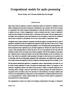
Fig. 1—(a) Solution of a four-component, 1D gas-injection problem and corresponding discrete points; (b) near-invariant path and corresponding discrete points. Reservoir temperature T 5 350 K; reservoir pressure p 5 100 bar; injection pressure pinj 5 130 bar; production pressure pprod 5 70 bar; injected composition is C4 (1%), C10 (1%), N2 (49%), CO2 (49%).

of the standard EOS-based model and two K-value models— namely, the standard (constant K-value) approach and the tie-linebased approach proposed here. Mathematical Model Conventional Compositional Approach. The full system of conservation equations that describes flow and transport of a multiphase multicomponent fluid can be written as ! X krj @ X ð/ xi; j qj sj Þ  r  xi; j qj k rp @s lj j j X xi; j qj qj ¼ 0; i ¼ 1; …; nc ;     ð1Þ þ j

xi; j 1i; j ðp; T; xj Þ  xi;k 1i;k ðp; T; xk Þ ¼ 0; i ¼ 0; …; nc ; 8j 6¼ k;                    ð2Þ nc X

xi; j  1 ¼ 0; j ¼ 1; …; np ; . . . ð3Þ

i¼1 np X

sj  1 ¼ 0: . . . . . . . . . . . . . ð4Þ

j¼1

The symbols are defined in the Nomenclature section. Here, we use the natural-variables formulation (Coats 1980), in which the nonlinear unknowns are p ¼ pressure, sj (np) ¼ vapor phase saturation, and xi, j (np  nc) ¼ phase composition of each component, i ¼ 1, …, nc in every phase j ¼ 1, …, np. The total number of unknowns (np  nc þ np þ 1) is equal to the total number of equations. Eq. 1 with p and xi, j (j is the index of an existing phase) as unknowns fully describes single-phase cells. For two-phase cells, the full system (Eqs. 1 through 4) with the complete set of nonlinear unknowns must be retained. For systems with more than two phases, the logic can be more complicated, but the idea of variable substitution remains the same. The general EOS-based compositional model has wide applicability; however, it has several disadvantages. First, rigorous phase-stability analysis and flash computations are iterative procedures that can consume significant computational time. Another problem is that the fugacity relations are highly nonlinear, and that makes it difficult to analyze the complex coupling of the thermodynamics with multiphase flow and multicomponent transport. The K-value model can improve the efficiency of the phasebehavior computation. Moreover, it provides a simpler form of December 2013 SPE Journal

the mathematical statement that facilitates detailed nonlinear analysis. Tie-Line-Based Parameterization. Here, we introduce a variable set based on tie-line (c) variables. We define the c-space as one space in which any point corresponds to one and only one tieline. It has been shown that with this variable set, we can split the problem of compositional flow simulation into thermodynamic and hydrodynamic parts (Entov 1997; Voskov and Entov 2001). Moreover, the solution of the thermodynamics problem is invariant to changes related to the hydrodynamics problem (Entov et al. 2001; Voskov and Tchelepi 2009b). Strict invariance has been proved under strong assumptions, but near-invariance was observed for more-general cases. If the thermodynamic state (chemical system and boundary conditions) is fixed, the projections of the solutions for various hydrodynamical properties, such as the permeabilities (both absolute and relative), and number of dimensions share a similar pattern in c-space (Entov 1997; Entov et al. 2001). We can take advantage of this near-invariance and generate K-value tables along the solution path to capture the important features of the displacement. To construct the path in c-space, we first solve a simple 1D problem for the given chemical system with boundary conditions (injection and initial composition and pressures) that are similar to the simulation model of interest. This full compositional solution of a 1D problem is then projected into c-space. This procedure is performed once only in a preprocessing stage. It has been shown that (Voskov and Tchelepi 2009c) for an overall composition z, we can find a unique tie-simplex (here, tie-line) that intersects the composition of interest, if we assume that the maximum number of phases is known. Here, we limit our study to two-phase hydrocarbon mixtures. Fig. 1 illustrates the approach with ci ¼ (xi þ yi)/2, i ¼ 1, 2. The solution of a four-component, 1D problem is shown in Fig. 1a; the projection of the solution into the c-space is shown in black in Fig. 1b. To illustrate the near-invariance of the c-path, we plot the solution of a 2D highly heterogeneous case [first layer of SPE10 model (Christie and Blunt 2001)] with the same chemical system and similar boundary conditions (blue dots). The figure indicates that the solutions are quite similar. The red circles on the c-path correspond to the compositions selected to build the tie-line tables. These points correspond to the major features of the solution structure (shocks and rarefactions) in Fig. 1a. K-Value Model Here, we describe the main principles of K-value approaches for two-phase systems, and we present the details of our tie-line1113

values during the simulation. The interpolation procedure is detailed in the next sections.

NC4

Subcritical Interpolation. As mentioned in the Introduction, once a set of compositions has been selected for building the Kvalue tables, there is no obvious criterion to choose which Kvalues should be used for a given gridblock. Here, the interpolation operator, LH, is constructed in two steps. First, we use a linear interpolation in pH and compute a new set of tie-lines at pressure p for all the compositions zj, j ¼ 1…Nz. Then, we find the closest two tie-lines in the set of interpolated tie-lines by computing d(z,p), which is the distance between the composition z of the gridblock and a tie-line, as follows: CO2

C10

Fig. 2—Phase envelope at low pressure (blue: T 5 470 K, p 5 30 bar) and at higher pressure (red: T 5 470 K, p 5 86 bar).

dðz; pÞ ¼ kz  x  Vðy  xÞk . . . . . . . . . . . . . . . . . . . ð6Þ Vðz; pÞ ¼

; T ðy X xÞ ðy  xÞ ; . . . . . . . . . . . . . . . . ð7Þ ðyc  xc Þðzc  xc Þ ¼ Xc ðy  xc Þðyc  xc Þ c c

based K-value method, which uses the concept of near-invariance presented in the preceeding section. Main Principles. K-value approaches use the following equation to describe the phase equilibrium: yi  xi Ki ¼ 0; i ¼ 1; …; nc : . . . . . . . . . . . . . . . . . . . . ð5Þ Here, we use the following notation: xi,g ¼ yi, and xi,1 ¼ xi, i ¼ 1, …, nc. On the basis of Eqs. 2 and 5, the K-value for the general equilibrium phase behavior is Ki ¼ fi,g/fi,1. The approach uses K-value tables that are precomputed for a discrete subset of the nonlinear unknowns (e.g., pressure and temperature) for the constant-Kvalue method. To capture the compositional dependence of the phase behavior, we need to find a way to include composition in the subset of nonlinear unknowns. A generalized K-value approach consists of the following steps:  For the full set of nonlinear unknowns, u (e.g., p, sg, and xi, j, with i ¼ 1, …, nc and j ¼ 1, …, np), introduce a new parameter space, v ¼ v(u); for the constant-K-value method, v  p; for our tie-line-based K-value method, v  p, z.  Choose a discrete subspace, vH, of the continuous space v; for the constant-K-value method, vH ¼ ( pi, i ¼ 1…Np); for our tieline-based K-value method, vH ¼ ( pi, i ¼ 1…Np; zi, i ¼ 1…Nz).  Construct K-value tables on the basis of KH ¼ K(vH) (preprocessing step).  Introduce an interpolation operator, LH, to provide a continuous representation K ¼ LH (KH). One way of defining the v space for isothermal problems is to choose v  p (constant-K-value method). This corresponds to linear boundaries of the two-phase region (Fig. 2, blue phase envelope), which is valid for hydrocarbon mixtures at low pressures. Assuming that the K-values depend only on pressure simplifies the problem; because pressure is a scalar, the interpolation of Kvalues is straightforward. However, for high pressures, the assumption of linear boundaries for the two-phase region is no longer valid (Fig. 1, red phase envelope). The critical point can appear inside the phase diagram, and the K-values become strong functions of composition, especially in the neighborhood of the critical point. The composition dependence of the K-values can no longer be ignored. This has two major consequences. First, in the subcritical region, the K-values have to be interpolated with respect to pressure and the vector of compositions, which makes the interpolation procedure complex. Second, in the supercritical region, there are no tie-lines and the Kvalues are trivial, which means that a criterion is needed to evaluate when a mixture enters or leaves the supercritical region. In the new approach, tie-line tables are generated for a uniform distribution of compositions selected along the near-invariant solution path zj, j ¼ 1…Nz. The total number of precomputed tielines is equal to NzNp. These tables are used to interpolate K1114

ðy  xÞT ðz  xÞ

where x and y are the endpoints of the interpolated tie-line at pressure p. Here, d(z, p) can be used as a weighting factor for linear interpolation of KH as a function of z; consequently, the derivatives @d/@zi can be computed and used to construct the part of the Jacobian matrix corresponding to Eq. 5. We use the two closest tie-lines to be consistent with the assumption that the solution follows a 1D path in c-space. We end up with dk ðz; pÞ ¼

rX ffiffiffiffiffiffiffiffiffiffiffiffiffiffiffiffiffiffiffiffiffiffiffiffiffiffiffiffiffiffiffiffiffiffiffiffiffiffiffiffiffiffiffiffiffiffiffiffiffiffiffiffiffiffiffiffiffiffiffiffiffiffiffiffi ½zic  xk;ic  Vðyk;ic  xk;ic Þ2 ic

vffiffiffiffiffiffiffiffiffiffiffiffiffiffiffiffiffiffiffiffiffiffiffiffiffiffiffiffiffiffiffiffiffiffiffiffiffiffiffiffiffiffiffiffiffiffiffiffiffiffiffiffiffiffiffiffiffiffiffiffiffiffiffiffiffiffiffiffiffiffiffiffiffiffiffiffiffiffiffiffiffiffiffiffiffiffiffiffiffiffiffiffiffiffiffiffiffiffiffiffiffiffiffiffiffiffiffiffiffiffiffiffiffiffiffiffiffi X " #2ffi u uX ðy  xk;c Þðzc  xk;c Þ t c k;c X zic  xk;ic  ¼ ðyk;ic  xk;ic Þ ðy  xk;c Þðyk;c  xk;c Þ ic c k;c k ¼ 1; 2;

                        ð8Þ

where x and y are the bubblepoints and dewpoints interpolated at pressure p, respectively. The index k ¼ 1 corresponds to the closest tie-line and k ¼ 2 to the second-closest tie-line; thus, d1(z,p) < d2(z, p). After the interpolation with respect to pressure, the bubblepoint composition at a given p is xk ðpÞ ¼

p2  p p  p1 x^k;p1 þ x^k;p2 ; . . . . . . . . . . . . . . ð9Þ p2  p1 p2  p1

where x^k;p1 and x^k;p2 are the tabulated bubblepoints at p1 and p2, respectively. After the interpolation with respect to composition, we have d1 ½x2 ðpÞ  x1 ðpÞ d1 þ d2 p2  p p  p1 ¼ x^1;p1 þ x^1;p2 p2  p1 p2  p1   d1 p2  p p  p1 þ x^2;p1 þ x^2;p2 d1 þ d2 p2  p1 p2  p1   p2  p p  p1 x^1;p1 þ x^1;p2 :        ð10Þ  p2  p1 p2  p1

xðp; zÞ ¼ x1 ðpÞ þ

We do the same thing for the dewpoint composition and construct K-values as follows: K(p, z) ¼ y(p, z)/x(p, z). Fig. 3a shows the solution (black) of a three-component gas displacement problem in which the phase behavior is described by a standard EOS approach. The solution was parameterized, and a discrete subspace, vH ¼ (pH, zH), was constructed. The blue and red dots correspond to stored tie-lines at pl and pu, respectively, where pl, pu 2 pH are the closest two pressures to the gridblock pressure p. The interpolated set of tie-lines (yellow circles) for p 2 (pl, pu) is shown in Fig. 3b. The black line is the phase diagram obtained by standard flash computation for pressure p. The December 2013 SPE Journal

NC4

NC4

C10

CO2 (a)

C10

CO2 (b)

Fig. 3—(a) Solution of a 1D problem and stored tie-lines at 70 bar (pl, blue dots) and 90 bar (pu, red dots); (b) interpolated endpoints of tie-line at 80 bar (yellow circles) and phase envelope at 80 bar.

TABLE 1—COST OF STABILITY VS. NUMBER OF POINTS SELECTED ALONG THE SOLUTION PATH Stability, % to EOS Number of Points Selected Along the Solution Path

Arithmetic Operations

Computation Time

5 10 20

4.9% 9.5% 18.6%

17.8% 19.3% 22.1%

interpolated tie-lines are in excellent agreement with the reference solution, even in the neighborhood of the critical point. We assume that the overall composition z of the gridblock under consideration is the green block shown in Fig. 3b, and that the pressure is p. To compute the K-value, we first interpolate a set of tie-lines at p (yellow circles), and we find the closest two tie-lines (green tie-lines). We use the distance between the composition and these two tie-lines to interpolate the K-values with respect to composition. We end up with K-values that are explicit functions of pressure and the compositions of all the components of the system. The number of points zj selected along the solution path has a direct effect on the performance of the method. Indeed, looking for the closest two tie-lines, which is performed during the phasestability analysis, requires that we go through the list of all the tielines. Thus, the cost of this operation is almost linear in the number of points zj, as shown in Table 1. The test case considered is a heterogeneous 2D miscible displacement (first layer of SPE10), and the cost of stability analysis is expressed in terms of number of arithmetic operations and computation time. Supercritical Interpolation. We now describe how our tie-linebased K-value method deals with supercritical mixtures, thus allowing for the simulation of miscible displacement processes. The approach makes use of the continuity of the tie-line length as a function of pressure and temperature for a given composition and uses the concept of the MCP suggested by Voskov and Tchelepi (2008). Any composition in the subcritical region is supported by (associated with) a tie-line, or its extension. As the pressure increases, the length l of the supporting tie-line decreases and becomes zero when the pressure reaches pmc, or the MCP for this composition, which we write as lim lðp; zÞ ¼ 0: . . . . . . . . . . . . . . . . . . . . . . . . . . ð11Þ

p!pmc

In a preprocessing step, the MCPs and the critical tie-lines for all the compositions selected to discretize v are computed. We December 2013 SPE Journal

start by flashing the composition of interest, z, at low pressure (negative flash), and we compute the tie-line length. As we increase the pressure, we monitor the length of the tie-line that supports z. When the tie-line length satisfies 1.10–3 < tie-line length < 3.10–2, the pressure is considered to be the MCP for z, and the tie-line is added to the critical-tie-line table. Note that there is only one pmc ¼ constant for the standard K(p) approach, whereas in our tie-line-based approach pmc depends on z for general nc-component mixtures. The total number of precomputed critical tie-lines is, at most, equal to Nz because some compositions can stay in the subcritical region for the entire pressure range. During a simulation run, we evaluate the distance between the gridblock composition and the closest critical tie-line. If this distance is less than a chosen e (here, we use e ¼ 510–2), we compare the pressure of the gridblock p with the MCP associated with the closest critical tie-line pmc(z). The mixture is considered supercritical if p > pmc(z), and we can use a simple correlation to determine whether the mixture is vapor- or liquid-like (CMG 2010; Schlumberger 2010). Alternatively, the critical tie-line on which z lies can be used to geometrically determine on which side of the phase envelope, liquid or gas, the composition z is. If p < pmc(z), the gridblock is subcritical, and we can use K-values to describe the phase behavior. The MCP criterion can be summarized as follows:  For all the parameters vH corresponding to changes in commc position, compute pmc H ¼ p ðvH Þ.  For a given composition z, evaluate its pmc by finding the closest critical tie-line.  If the distance between z and the closest critical tie-line is less than e, compare pmc(z) with the pressure of the gridblock. Voskov and Tchelepi (2008, 2009a) showed that interpolation close to the MCP can lead to large errors because the tie-line length changes rapidly to zero in the neighborhood of pmc. As explained in the preceding subsection, the K-value associated with z and p is interpolated by use of the closest two pressures, p1 and p2, and the closest two tie-lines in a new set of tie-lines interpolated at pressure p. When interpolating a new tie-line associated with composition zj at pressure p, large errors may be obtained if p1 < pmc(zj) < p2 because zj is subcritical at p1 but supercritical at p2 and is no longer supported by a tie-line. This error will have an effect on the final result if this interpolated tie-line happens to be one of the two closest ones, which can occur when z is in the neighborhood of the critical point. This is why the interpolation operator uses p2 ¼ pmc(zj) (Eq. 10) and the critical tie-line associated with zj when the mixture is near the critical point. The concept of MCP is closely related to the concept of convergence pressure. If we plot the K-values as a function of pressure for a given composition, we observe that they converge to unity at the so-called convergence pressure. Convergence pressures have been used to tabulate K-values in an effort to capture some of the composition dependence of phase behavior [the 1115

Saturation of the gas phase (EOS model) 60 40

NC4

0.5

20

60

50 100 150 200 Error: saturation (generalized K-value)

40

C1

60

50 100 150 200 Error: saturation (standard K-value)

40 CO2

0.2

0 0.2 0.1

20 50

(a)

0

0.1

20 C10

1

100

150

200

0

(b)

Fig. 4—(a) Case 1: solution path in compositional space (p 5 165 bar, T 5 345 K); (b) gas-phase saturation at the end of the simulation and absolute error obtained with K-value methods.

K-value tables published by the Gas Processor Suppliers Association (GPSA 2004) are considered to be the most extensive set of published equilibrium ratios for hydrocarbons]. Because the convergence pressure of a given composition is not known a priori, an iterative process or a simplified correlation is required to use such tabulated K-values (Hagoort 1988). In contrast, the MCP of a given composition is evaluated directly by finding the closest critical tie-line in the set of preprocessed critical tie-lines. Moreover, MCPs are not used to capture the composition dependence of phase behavior, but only to detect when a mixture enters or leaves the supercritical region. Numerical Implementation. The algorithms of the two main parts of our tie-line-based K-value method are given in Algorithm 1 (stability test) and Algorithm 2 (computation of fluid properties). Algorithm 1. Phase stability, tie-line-based K-value method. 1: if first Newton iteration, or gridblock in a single-phase state, then 2: find and save closest two pressures, pl and pu, 3: find distance d between z and closest critical tie-line, TLcritical, 4: save pmc(z) ¼ pmc(TLcritical); 5: if d < e and p  pmc(z), then 6: the mixture is supercritical; 7: evaluate whether the mixture is gas-like or liquid-like, 8: else 9: the mixture is subcritical 10: end if 11: if mixture is subcritical, then 12: interpolate set of tie-lines with respect to p; 13: find and save closest two tie-lines (zl and zu) and compute distances dl and du, 14: interpolate K-values with respect to composition, 15: solve Rachford-Rice equation, 16: evaluate whether a phase is stable or not by use of phase fractions, 17: compute x and y if needed, 18: end if 19: end if. Algorithm 2. Phase properties, tie-line-based K-value method. 1: if gridblock in two-phase state, then 2: extract closest two pressures (pl, pu) and tie-lines (compositions) (zl, zu) saved during stability test, 3: re-evaluate distances between z and closest two tie-lines, 4: interpolate K-values with respect to p and z, 1116

5: build equation: yi – xiKi ¼ 0, i ¼ 1, …, nc, 6: end if. Results We present results for miscible and immiscible displacements. Three different formulations are used: a standard EOS-based compositional model; our K-value model, K ¼ K( p, z), on the basis of tie-line parameterization computed from a simple 1D solution; and the standard constant-K-value model, K ¼ K( p). For the constantK-value method, the K-values are computed for an average composition of the initial and injected compositions. By doing so, we minimize the error obtained with the constant-K-value method. For the tie-line-based K-value method, a critical tie-line is considered to intersect a composition z, if the distance between z and the critical tie-line is less than 510–2. We report the total number of tie-lines precomputed, which includes the critical tie-lines. 2D Simulations. The permeability and porosity fields are taken from the top layer of the SPE10 model (Christie and Blunt 2001). Case 1: Four Components, 2D, Multicontact Miscible Displacement. A gas mixture of [C1 (11%), C10 (1%), C4 (23%), CO2 (65%)] is injected into oil made up of [C1 (55%), C10 (43%), C4 (1%), CO2 (1%)]. Injection and production wells operate at bottomhole pressure (BHP) of p ¼ 180 and p ¼ 145 bar, respectively. One injection well is at the center of the reservoir, and four production wells are in the corners. The reservoir temperature T is 345 K, and the initial reservoir pressure is p ¼ 160 bar. Fig. 4a shows the 1D solution obtained in the preprocessing stage. Fig. 4b shows the saturation of the gas phase at the end of the simulation (5,000 days) and the absolute error obtained with the K-value methods. A total of 120 tie-lines were precomputed for the tieline-based K-value method. Case 2: Four Components, 2D, Immiscible Displacement. A gas mixture of [N2 (49%), C10 (1%), C4 (1%), CO2 (49%)] is injected into oil made up of [N2 (1%), C10 (9%), C4 (89%), CO2 (1%)]. Injection and production wells operate at BHP of p ¼ 130 and p ¼ 70 bar, respectively, and are at opposite corners. The reservoir temperature is T ¼ 350 K, and the initial reservoir pressure is p ¼ 100 bar. Fig. 5a shows the 1D solution obtained in the preprocessing stage. Fig. 5b shows the saturation of the gas phase at the end of the simulation (5,000 days) and the absolute error obtained with the K-value methods. A total of 110 tie-lines were precomputed for the tie-line-based K-value method. Case 3: Nine Components, 2D, Immiscible Displacement. Two different gas mixtures are injected into oil made up of [CO2 (1%), C1 (19%), C2 (5%), C3 (5%), NC4(10%), NC5 (10%), C6 December 2013 SPE Journal

Saturation of the gas phase (EOS model) 60 NC4

40 20

60

50 100 150 200 Error: saturation (generalized K-value)

40

C10 60

0.2 0.1

20 N2

0.8 0.6 0.4 0.2 0

0

50 100 150 200 Error: saturation (standard K-value)

0.2

40 CO2

0.1

20 50

(a)

100

150

0

200

(b)

Fig. 5—(a) Case 2: solution path in compositional space (p 5 92 bar, T 5 350 K); (b) gas-phase saturation at the end of the simulation and absolute error obtained with K-value methods.

(10%), C8 (20%), C10 (20%)]. The compositions of the injected mixtures are [CO2 (83%), C1 (10%), C2 (1%), C3 (1%), NC4 (1%), NC5 (1%), C6 (1%), C8 (1%), C10 (1%)] and [CO2 (43%), C1 (50%), C2 (1%), C3 (1%), NC4 (1%), NC5 (1%), C6 (1%), C8 (1%), C10 (1%)]. Injection and production wells operate at BHP of p ¼ 120 and p ¼ 30 bar, respectively. Injection wells are close to the center of the reservoir and close enough to each other to force the streams to mix, and production wells are in the corners. The reservoir temperature is T ¼ 350 K, and the initial reservoir pressure is p ¼ 75 bar. Two 1D simulations were used to find the representative composition paths, one for each injected composition. Fig. 6 shows the saturation of the gas phase at the end of the simulation (2,000 days) and the absolute error obtained with the

K-value methods. A total of 200 tie-lines were precomputed for the tie-line-based K-value method. Case 4, Nine Components, 2D, Multicontact Miscible Displacement. A gas mixture of [CO2 (83%), C1 (10%), C2 (1%), C3 (1%), NC4 (1%), NC5 (1%), C6 (1%), C8 (1%), C10 (1%)] is injected into oil made up of [CO2(1%), C1 (19%), C2 (5%), C3 (5%), NC4 (10%), NC5 (10%), C6 (10%), C8 (20%), C10 (20%)]. Injection and production wells operate at BHP of p ¼ 130 and p ¼ 10 bar, respectively. Injection wells are close to the center of the reservoir and close enough to each other to force the streams to mix, and production wells are in the corners. The reservoir temperature is T ¼ 500 K, and the initial reservoir pressure is p ¼ 75 bar. Fig. 7 shows the saturation of the gas phase at the end of the

Saturation of the gas phase (EOS model) 60

0.8

50 40

0.6

30

0.4

20

0.2

10 20

40

60

80

100

120

140

160

180

200

220

0

Error: saturation (generalized K-value) 60

0.2

50

0.15

40 30

0.1

20

0.05

10 20

40

60

80

100

120

140

160

180

200

220

0

Error: saturation (standard K-value) 60

0.2

50

0.15

40 30

0.1

20

0.05

10 20

40

60

80

100

120

140

160

180

200

220

0

Fig. 6—Case 3: gas-phase saturation at the end of the simulation and absolute error obtained with K-value methods. December 2013 SPE Journal

1117

Saturation of the gas phase (EOS model) 60

0.8

50 40

0.6

30

0.4

20

0.2

10 20

40

60

80

100

120

140

160

180

200

220

0

Error: saturation (generalized K-value) 0.2

60 50 40 30 20 10

0.15 0.1 0.05 20

40

60

80

100

120

140

160

180

200

220

0

Error: saturation (standard K-value) 0.2

60 50 40 30 20 10

0.15 0.1 0.05 20

40

60

80

100

120

140

160

180

200

220

0

Fig. 7—Case 4: gas-phase saturation at the end of the simulation and absolute error obtained with K-value methods.

simulation (500 days) and the absolute error obtained with the Kvalue methods. A total of 100 tie-lines were precomputed for the tie-line-based K-value method. 3D Simulations. The permeability and porosity fields are taken from the top 10 layers of the SPE10 model (Christie and Blunt 2001). Two different compositions are injected, the wells perforate the 10 layers, and there is a gradient in the initial composition. The details of the test case are as follows:

Case 5: Four Components, 3D, Immiscible Displacement. As described in Fig. 8, two different gas mixtures are injected into oil made up of, on average, [C1 (30%), C10 (36%), C4 (33%), CO2 (1%)]. The distribution of the initial composition in the zdirection follows a compositional gradient, with zjl1: [C1 (40%), C10 (29%), C4 (30%), CO2 (1%)] and zjl10: [C1 (20%), C10 (43%), C4 (36%), CO2 (1%)]. The compositions of the injected mixtures are [C1 (19%), C10 (1%), C4 (1%), CO2 (79%)] at the first injection well and [C1 (79%), C10 (1%), C4 (1%), CO2 (19%)] at the

Injector 2 Injector 1 C1(79%), C10(1%), C4(1%), CO2(19%),

C1(19%), C10(1%), C4(1%), CO2(79%),

Producer 2 Producer 1

Initial compositional gradient z = 0: C1(40%), C10(29%), C4(30%), CO2(1%), z = –10: C1(20%), C10(43%), C4(36%), CO2(1%),

Fig. 8—Case 5: 3D simulation settings. 1118

December 2013 SPE Journal

60

60

40

40

20 60

20 50

100

150

01 200

40

50

100

150

60 40

20

20 50

100

150

05 200

40

02 200

50

100

150

04 200

60

0.8 0.6 0.4

50

100

150

06 200

50

100

150

08 200

50

100

150

10 200

0.2 0

40

20 60

150

20 03 200

40

60

100

40

20 60

60

50

20 50

100

150

07 200

40

60 40

20

20 50

100

150

09 200

Fig. 9—Case 5: gas-phase saturation at the end of the simulation.

second. The injection and production wells operate at BHP of p ¼ 100 and p ¼ 50 bar, respectively. Injection wells are on the left two corners, and the production wells are on the right two corners. The reservoir temperature is T ¼ 350 K, and the initial reservoir pressure is p ¼ 70 bar. Two 1D simulations were used to find representative composition paths, one for each injected composition. Fig. 9 shows the saturation of the gas phase at the end of the simulation (500 days), and Figs. 10 and 11 show the absolute error obtained with the K-value methods (the layers are ordered from top to bottom). 200 tie-lines were precomputed for the tieline-based K-value method. 60

60

40

40 20

20 60

50

100

150

01 200

60

50

100

150

03 200

60

40

40

20

20 50

100

150

05 200

150

02 200

50

100

150

04 200

60

0.2

0.1 50

100

150

06 200

50

100

150

08 200

50

100

150

10 200

0

40

40

20

20 60

100

20

20

60

50

40

40

60

Analysis of the Results. Cases 1 and 4 are multicontact miscible displacements, so the mixtures in parts of the reservoir are supercritical. Our tie-line-based K-value method uses the MCP criterion described previously to capture the transition between the subcritical and supercritical regions. The method predicts the locations of the gas front accurately and is in good agreement with the reference EOS-based results. The standard K-value model can capture the one MCP used in its construction, but is unable to capture the transition from supercritical to subcritical accurately. Case 2 is an immiscible displacement. Here, we focus on the composition dependence of phase behavior in the subcritical

50

100

150

07 200

60 40

40

20

20 50

100

150

09 200

Fig. 10—Case 5: absolute error obtained with our tie-line-based K-value method. December 2013 SPE Journal

1119

60

60

40

40

20 60

20 50

100

150

01 200

40

50

100

150

60

40

40 20 50

100

150

05 200

40

02 200

50

100

150

04 200

60

0.2

0.1 50

100

150

06 200

50

100

150

08 200

50

100

150

10 200

0

40

20 60

150

20 03 200

20 60

100

40

20 60

60

50

20 50

100

150

07 200

40

60 40

20

20 50

100

150

09 200

Fig. 11—Case 5: absolute error obtained with a constant-K-value method.

TABLE 2—MAXIMUM ERROR IN OIL-PRODUCTION RATE Case 1 2 3 4 5

K-Value Standard

K-Value Tie-Line

14.3% 15.0% 10.0% 18.7% 2.6%

1.8% 0.9% 1.9% 7.6% 0.4%

region that is significant for this system. We observe that our tieline-based approach captures accurately this composition dependence, whereas the constant-K-value approach gives large errors. Cases 3 and 5 are immiscible displacements with nine and four components, respectively. These cases show how our tie-line-based

method can be used with different injected compositions and, for Case 5, with an initial composition gradient in the reservoir. The method uses two 1D-solution paths. Here also our tie-line-based Kvalue method captures accurately the composition dependence of phase behavior, whereas the constant-K-value method does not. Table 2 compares the maximum error in oil-production rate obtained with the two K-value methods and for the five test cases considered. We observe that the tie-line-based K-value method is superior to the constant-K-value method at predicting production rates. As expected, the differences between the two K-value methods are more important for systems with stronger compositional dependence of phase behavior. Table 3 compares the performances of the different approaches considered. Here, we focus on the two parts of the code related to phase-behavior computation: phase-stability and fluid-property calculation. Table 3 presents the cost in terms of computation time and the number of nonlinear iterations of the flow and transport

TABLE 3—PERFORMANCE OF DIFFERENT APPROACHES: COMPUTATION TIME

Test Case 1, 2D

Case 2, 2D

Case 3, 2D

Case 4, 2D

Case 5, 3D

1120

Methods

Newton, Iterations

Total, seconds

Properties, seconds (Ratio)

Stability, seconds (Ratio)

EOS-Based Model K-Value Standard K-Value Tie-Line EOS-Based Model K-Value Standard K-Value Tie-Line EOS-Based Model K-Value Standard K-Value Tie-Line EOS-Based Model K-Value Standard K-Value Tie-Line EOS-Based Model K-Value Standard K-Value Tie-Line

16,467 690 593 566 577 555 256 254 243 399 272 286 1,783 1,787 1,024

28,879 496 1095 385 299 288 578 472 482 776 335 462 14,101 13,113 8,441

9,649 (33.4%) 180 (36.3%) 445 (40.7%) 85 (22.1%) 84 (28.1%) 88 (30.5%) 144 (24.9%) 142 (30.1%) 154 (31.9%) 312 (40.2%) 141 (41.9%) 211 (45.6%) 3,715 (26.4%) 3,571 (27.1%) 2,347 (27.8%)

4,798 (16.6%) 17 (3.4%) 33 (3.0%) 107 (27.8%) 18 (6.0%) 9 (3.1%) 111 (19.2%) 13 (2.7%) 9 (1.9%) 26 (3.4%) 4 (1.1%) 7 (1.6%) 982 (7.0%) 309 (2.3%) 270 (3.2%)

December 2013 SPE Journal

TABLE 4—POTENTIAL PERFORMANCE OF DIFFERENT APPROACHES: ARITHMETIC OPERATIONS

Test

Methods

Case 1, 2D

K-Value Standard K-Value Tie-Line K-Value Standard K-Value Tie-Line K-Value Standard K-Value Tie-Line K-Value Standard K-Value Tie-Line K-Value Standard K-Value Tie-Line

Case 2, 2D Case 3, 2D Case 4, 2D Case 5, 3D

Average EOS Iterations

Stability, % to EOS

Properties, % to EOS

16.7 SSI þ 2 Newton

0.6% 9.5% 0.9% 14.0% 0.9% 14.9% 0.5% 6.0% 1.3% 21.2%

2.4% 8.8% 2.4% 8.8% 1.5% 5.5% 1.5% 5.5% 2.4% 8.8%

12.6 SSI þ 2 Newton 9.4 SSI þ 2 Newton 23.4 SSI þ 2 Newton 7.1 SSI þ 2 Newton

problem, with the percentage to the total computation time in parentheses. With a K-value model, we are able to reduce the time spent on phase-behavior computation quite substantially. As expected, the computational cost increases as the complexity of the K-value model increases. However, the standard K-value model fails to capture the important features associated with the true solution. For example, in Case 2, the standard K-value method solves a completely different and wrong problem (immiscible displacement). The total simulation times of the tie-line-based Kvalue method reported in Table 3 do not include the preprocessing step, which has not been automated yet. However, the main part of this preprocessing step consists of solving a 1D problem. For all the cases presented in this paper, these 1D simulations take a few seconds: Case 1 (13.2 seconds), Case 2 (4.2 seconds), Case 3 (9.0 seconds), Case 4 (4.0 seconds), and Case 5 (5.9 seconds). The cost of the stability analysis in our tie-line-based K-value model depends on the number of points selected along the solution path(s), zj. As explained previously, we need to find the closest two tie-lines to z, and therefore, we need to evaluate d(z, p) for each zj. Our computational experience indicates that the relationship between the number of selected points, zj, and the cost of stability analysis is nearly linear, as shown in Table 1. Likewise, we observe in Tables 3 and 4 that increasing the number of components (from four to nine) does not dramatically increase the cost of the phase-stability analysis. This is because the cost of interpolation increases linearly with the number of components. The new K-value method has been implemented in our general-purpose research simulator—AD-GPRS—which is built on top of an automatic differentiation with expression templates library (ADETL), described in Younis and Aziz (2007) and Younis (2011). Automatic differentiation (AD) can generate the corresponding derivatives for the nonlinear relation of choice, which greatly simplifies the computation of the Jacobian. For the tieline-based K-value method, fluid-property calculations include bilinear interpolation of K-values, which are used in place of fugacities to construct the phase-equilibrium equation. Because their derivatives are used in the Jacobian matrix, K-values have to be interpolated as AD variables. This introduces additional overhead for K-value models caused by extra computation of these derivatives. The interpolation of K-values as AD variables consists in updating the distances d(z, p) between the composition z and the closest two tie-lines before carrying out the bilinear interpolation with respect to pressure and composition. In our current implementation, the fluid density q and viscosity l are computed by use of an EOS. However, in a K-value model, all the properties can be evaluated by linear interpolation, as well. Moreover, the interpolation coefficients used for K-values can also be used to interpolate the other properties. By doing so, we can improve the performance even more. In Table 4, we present the potential performance of the methods evaluated by the average number of arithmetic operations per nonlinear iteration and per block needed for the stability check and fluid-property calcuDecember 2013 SPE Journal

lations. Here, all the fluid properties for the tie-line-based K-value method are considered to be interpolated, and the reference is the number of operations required by the EOS-based model. In the same table, we can see that the stability analysis in a K-value model requires fewer iterations than in an EOS-based model. Indeed, whereas the stability analysis based on an EOS is an iterative process, which consists of a successive-substitution-iteration (SSI) algorithm followed by a Newton-based solver, the stability analysis in a K-value model does not require iteration. Conclusions We presented a tie-line-based K-value method for generalpurpose compositional simulation. This method can be used to improve any existing K-value-based model by introducing only one additional degree of freedom to capture complicated compositional effects. Specifically, the proposed approach captures the composition dependence of the phase behavior for multicomponent mixtures and the important features of near-miscible gas displacement processes. We compared the tie-line-based K-value model with the standard K-value approach and the fully EOSbased compositional model for several challenging examples. The results indicate that the tie-line-based K-value approach leads to robust and efficient computations of the phase behavior associated with compositional flow simulation. We introduced a criterion based on the concept of MCP that captures the transition between the super- and subcritical regions. The combination of composition-dependent K-values with this criterion allows us to use the Kvalue approach for near-miscible displacement simulation. The proposed method can be implemented in existing K-value-based simulators relatively easily, and that extends the ability of such simulators to model near-miscible displacement processes. Nomenclature d ¼ distance between a composition and a tie-line k ¼ absolute-permeability tensor [L2] KH ¼ K-value tables krj ¼ phase relative permeability l ¼ length of a tie-line LH ¼ interpolation operator p ¼ pressure [M/LT2] (bar) pmc ¼ minimal critical pressure (MCP) [M/LT2] (bar) qj, j ¼ 1, … np ¼ fluid-phase source [T1] sg ¼ vapor-phase saturation sj, j ¼ 1, … np ¼ phase saturations u ¼ nonlinear unknowns xi, i ¼ 1, … nc ¼ liquid-phase concentration of component i xi, j, i ¼ 1, … nc, j ¼ 1, … np ¼ concentration of component i in phase j 1121

yi, i ¼ 1, … nc ¼ gas-phase concentration of component i ci ¼ variable in tie-line space fi, j ¼ fugacity coefficient of component i in phase j lj ¼ phase viscosity [ML1T1] qj, j ¼ 1, … np ¼ phase molar density [NL3] / ¼ porosity

Acknowledgments Thanks to Total and the SUPRI-B Industrial Affiliates program on reservoir simulation at Stanford University for financial support. References Aziz, K. and Wong, T. 1988. Considerations in the Development of Multipurpose Reservoir Simulation Models. Proc., 1st and 2nd International Forum on Reservoir Simulation, Alpbach, Austria. Bedrikovetsky, P. and Chumak, M. 1992. Riemann Problem for TwoPhase Four- and More Component Displacement (Ideal Mixtures). Proc., Third European Conference on the Mathematics of Oil Recovery (ECMOR), Delft, the Netherlands, 139–148. Bolling, J. 1987. Development and Application of a Limited-Compositional, Miscible Flood Reservoir Simulator. Paper SPE 15998 presented at the SPE Symposium on Reservoir Simulation, San Antonio, Texas, 1–4 February. http://dx.doi.org/10.2118/15998-MS. Christie, M. and Blunt, M. 2001. Tenth SPE Comparative Solution Project: A Comparison of Upscaling Techniques. SPE Res Eval & Eng 4 (4): 308–317. http://dx.doi.org/10.2118/72469-PA. Computer Modelling Group (CMG). 2010. STARS User’s Guide. Calgary, Alberta: CMG. Coats, K. 1980. An Equation of State Compositional Model. SPE J. 20 (5): 363–376. http://dx.doi.org/ 10.2118/8284-PA. Entov, V. 1997. Nonlinear Waves in Physicochemical Hydrodynamics of Enhanced Oil Recovery. In Multicomponent Flows: Proceedings of the International Conference Porous Media: Physics, Models, Simulations, Moscow, Russia. Entov, V., Turetskaya, F. and Voskov, D. 2001. On Approximation of Phase Equilibria of Multicomponent Hydrocarbon Mixtures and Prediction of Oil Displacement by Gas Injection. Oral presentation given at the 8th European Conference on the Mathematics of Oil Recovery, Freiburg, Germany, 4–7 September. Gas Processor Suppliers Association (GPSA). 2004. Gas Processors Suppliers Association Engineering Data Book, twelfth edition. Tulsa, Oklahoma: Gas Processor Suppliers Association. Hagoort, J. 1988. Fundamentals of Gas Reservoir Engineering. Amsterdam, the Netherlands: Elsevier Science Publishers. Hand, D. 1930. The Distribution of a Consolute Liquid Between Two Immiscible Liquids. J. Phys. Chem. 34 (9): 1961–2000. http://dx.doi.org/ 10.1021/j150315a009. Iranshahr, A., Voskov, D. and Tchelepi, H. 2010. Tie-Simplex Parameterization for EOS-Based Thermal Compositional Simulation. SPE J. 15 (2): 537–548. http://dx.doi.org/10.2118/119166-PA. Landmark Graphics Corporation. 2001. VIP Technical Reference. Houston, Texas: Landmark. Orr, F. M. 2007. Theory of Gas Injection Processes. Holte, Denmark: TieLine Publications. Rannou, G., Voskov, D. and Tchelepi, H. 2010. Extended K-Value Method for Multi-Contact Miscible Discplacements. Proc., 12th European Conference on the Mathematics of Oil Recovery, Oxford, UK. Roshanfekra, M., Li, Y. and Johns, R. 2010. Non-Iterative Phase Behavior Model with Application to Surfactant Flooding and Limited Compositional Simulation. Fluid Phase Equilib. 289 (2): 166–175. http:// dx.doi.org/10.1016/j.fluid.2009.11.024.

1122

Schlumberger. 2010. ECLIPSE User’s Guide. Houston, Texas: Schlumberger. Tang, D. and Zick, A. 1993. A New Limited Compositional Reservoir Simulator. Paper SPE 25255 presented at the SPE Symposium on Reservoir Simulation, New Orleans, Louisiana, 28 February–3 March. http://dx.doi.org/10.2118/25255-MS. Todd, M. and Longstaff, W. 1972. The Development, Testing, and Application Of a Numerical Simulator for Predicting Miscible Flood Performance. J Pet Tech 24 (7): 874–882. http://dx.doi.org/10.2118/3484-PA. Van-Quy, N., Simandoux, P. and Corteville, J. 1972. A Numerical Study of Diphasic Multicomponent Flow. SPE J. 12 (2): 171–184. http:// dx.doi.org/10.2118/3006-PA. Voskov, D. and Entov, V. 2001. Problem of Oil Displacement by Gas Mixtures. Fluid Dyn. 36 (2): 269–278. http://dx.doi.org/10.1023/ A:1019290202671. Voskov, D. and Tchelepi, H. 2008. Compositional Space Parametrization for Miscible Displacement Simulation. Transport Porous Med. 75 (1): 111–128. http://dx.doi.org/10.1007/s11242-008-9212-1. Voskov, D. and Tchelepi, H. 2009a. Compositional Space Parameterization: Multicontact Miscible Displacements and Extension to Multiple Phases. SPE J. 14 (3): 441–449. http://dx.doi.org/10.2118/113492-PA. Voskov, D. and Tchelepi, H. 2009b. Compositional Space Parameterization: Theory and Application for Immiscible Displacements. SPE J. 14 (3): 431–440. http://dx.doi.org/10.2118/106029-PA. Voskov, D. and Tchelepi, H. 2009c. Tie-Simplex Based Mathematical Framework for Thermodynamical Equilibrium Computation of Mixtures with an Arbitrary Number of Phases. Fluid Phase Equilib. 283 (1–2): 1–11. http://dx.doi.org/10.1016/j.fluid.2009.04.018. Young, L. and Stephensen, R. 1983. A Generalized Compositional Approach for Reservoir Simulation. SPE J. 23 (5): 727–742. http:// dx.doi/org/10.2118/10516-PA. Younis, R. 2011. Modern Advances in Software and Solution Algorithms for Reservoir Simulation. PhD dissertation, Stanford University, Stanford, California (August 2011). Younis, R. and Aziz, K. 2007. Parallel Automatically Differentiable DataTypes for Next-Generation Simulator Development. Paper SPE 106493 presented at the SPE Reservoir Simulation Symposium, Houston, Texas, 26–28 February. http://dx.doi.org/10.2118/106493-MS. Guillaume Rannou holds master’s degrees in mechanical engineering from E´cole Nationale Supe ´ rieure d’Arts et Me ´ tiers, Paris, France, and from the Georgia Institute of Technology, Atlanta, Georgia. He spent 2 years as a visiting researcher in the Department of Energy Resources Engineering at Stanford University, Stanford, California, where he focused on new approaches for compositional simulation. Rannou now works for Schlumberger as a software engineer in Abingdon, UK. Denis Voskov is a senior research associate at Stanford University and leads the research on thermal simulation in the Department of Energy Resources Engineering at Stanford. His research covers new approaches for compositional modeling; simulation of advanced thermal processes; analysis and improvement of nonlinear solvers for complex physical systems; general-purpose simulation of multiphase multicomponent flow in porous media; multiscale compositional modeling; modeling of CO2-sequestration processes; and adjoint-based optimization. Hamdi Tchelepi is a professor at Stanford University and codirector of the Center for Computational Earth and Environmental Science. His research covers various aspects of numerical modeling of flow and transport in natural porous media. Specific interests include analysis of unstable miscible and immiscible flows in heterogeneous formations; scalable (efficient for large problems) linear and nonlinear solution algorithms of multiphase flow in highly heterogeneous systems; and stochastic moment equation methods for quantifying the uncertainty associated with predictions of flow performance in the presence of limited reservoir-characterization data.

December 2013 SPE Journal