Dec 15, 2004 - Tight-binding calculations of NMR transitions in random and ... Physics Department, University of Utah, Salt Lake City, Utah 84112, USA.
PHYSICAL REVIEW B 70, 224207 (2004)
Tight-binding calculations of NMR transitions in random and partially ordered GaInP2 C. B. Nelson and P. C. Taylor Physics Department, University of Utah, Salt Lake City, Utah 84112, USA
W. A. Harrison Department of Applied Physics, Stanford University, Stanford, California 94305, USA (Received 5 February 2004; revised manuscript received 16 August 2004; published 15 December 2004) A tight-binding method is used to obtain the average local order parameter for random and partially ordered GaInP2 from the electric field gradients (EFG’s) at Ga sites. The EFG’s are obtained from 71Ga nuclear magnetic resonance (NMR). The calculations employed a 17-atom cluster consisting of a central Ga, 4 nearestneighbor P, and 12 second-nearest-neighbor Ga or In atoms. In partially ordered GaInP2 there are 8192 such clusters. Distortions from perfect tetrahedral symmetry are obtained using a force balance method with an undistorted bond length of 2.45 Å (average lattice approximation). Comparisons with the NMR data are obtained for a sample grown by liquid phase epitaxy (LPE), which approximates a random sample, and for a sample grown by organometallic vapor phase epitaxy (OMVPE), which is partially ordered. The random assumption provides good agreement with experiment for the LPE sample, and a least-squares fit to the data for the OMVPE sample yields a local order parameter of 0.4± 0.1. DOI: 10.1103/PhysRevB.70.224207
PACS number(s): 71.15.Ap, 31.15.Ct, 76.60.Gv
I. INTRODUCTION
Partial ordering of the mixed cation or anion sublattices in ternary III-V semiconductors has been the subject of much investigation. The usual methods for determining the local order parameter have been optical measurements combined with models of the optical transitions. The atomic ordering phenomenon1–5 occurs in many ternary and quaternary semiconductors grown by the organometallic vapor phase epitaxy (OMVPE) method.6–14 GaInP2 is perhaps the best-studied, ternary III-V alloy that orders. The atoms in GaInP2 have tetrahedral configurations, and when the material is grown using the OMVPE method spontaneous ordering can occur along a specific direction, often along a 关111b兴 direction.11,15 In this case, gallium-rich [111] planes are followed by phosphorus planes, indium-rich planes, and phosphorus planes, respectively. Then the cycle repeats. In the case of perfect ordering this arrangement produces a socalled monolayer superlattice with long-range order. In practical situations the ordering occurs as atomic surfaces are formed16 and is not perfect in the sense that each gallium- or indium-rich plane always contains atoms of the other cation species. The degree of local ordering can be quantified by defining a local order parameter , which is the number of cations of the dominant type minus the number of the second cation normalized by the total number of cations in the plane. For the long-range order parameter one must average the local order parameter over many planes. The most common type of ordering that occurs in GaInP2 is the so-called copper platinum structure, which is ordered along the 关111b兴 direction and is the most studied in the literature.1 Spontaneous ordering changes many experimentally observable electronic and optical properties. Examples of these are band-gap reduction,16 valence-band splitting,17,18 optical 1098-0121/2004/70(22)/224207(10)/$22.50
anisotropy,17 pyroelectricity,19 birerefringence,20 secondharmonic generation,21 conductivity anisotropy,22 and reduction of alloy fluctuations.23 Accurate measurement of the average local order parameter for a given sample is crucial if one wishes to understand the dependences of the above properties on the degree of order. Many authors have used pseudopotential methods to calculate the order parameter. Mader and Zunger24 used a pseudopotential method and valence forces to determine that the optical band-gap reduction is proportional to the square of the order parameter, ⌬Egap ⬀ 2 ,
共1兲
where Egap is the energy gap and is the long-range order parameter. The results of Mader and Zunger24 are shown as the short-dashed line in Fig. 1. The bond lengths calculated for random GaInP2 are in excellent agreement with x-ray absorption fine structure measurements.25–27 Zhang et al.28 have made the claim that this dependence is too simple and that the band-gap reduction should also depend on higherorder terms in . These authors applied a modified empirical pseudopotential method to calculate the band structure of partially ordered GaInP2 for any given order parameter. Wei et al.29 developed a statistical description of the possible configurations of GaInP2 using an Ising model (long-dashed line in Fig. 1). The band-gap reduction as a function of shortrange order calculated by these authors has the same form as in Eq. (1) and is in agreement with the polarized photoluminescence results of Kanata et al.30 and the polarized electromodulation results of Glembocki et al.31 More recently Forrest et al.32 have employed an x-ray technique to measure directly the order parameter in highly ordered samples of GaInP2. This method is based on the idea that ordered regions produce extra x-ray reflections. For the CuPt structure ordering occurs in the 兵1 , 1 , n其 planes (see Fig. 2), producing 兵1 / 2 , 1 / 2 , n / 2其 superlattice reflections.32
224207-1
©2004 The American Physical Society
PHYSICAL REVIEW B 70, 224207 (2004)
NELSON, TAYLOR, AND HARRISON
FIG. 1. Solid circles: long-range order parameters for six samples of OMVPE grown, highly ordered GaInP2 calculated from x-ray measurements (Ref. 32). Note the maximum order is approximately equal to 0.5. Short-dashed line: model calculation from Ref. 24. Note the 2 dependence. Long-dashed line: model calculation from Ref. 29. Solid line: model calculation from Ref. 28. The solid square with the large error bar is the result from the present calculation as described in the text.
The integrated Bragg intensity from a periodic crystal is proportional to the magnitude of the crystal structure factor, I ⬀ 兩Ft兩2. The structure factor Ft for CuPt-ordered GaInP2 includes both fundamental zinc-blende reflections {113} and superstructure reflections resulting from CuPt long-range order, {1/2,1/2,3/2}. The structure factor can be written in terms of the order parameter . These authors32 calculated the degree of order by comparing the ratio of the integrated Bragg intensities of the four {1/2,1/2,3/2} superlattice peaks
to the corresponding Bragg intensities of the {113} fundamental peaks. The curve of Ref. 24 provides the best agreement with the x-ray32 data. The accuracy of this calculation depends partially on the atomic scattering factors, which were modified using standard corrections33 for dispersion and thermal vibration (using Debye-Waller factors). This method is the simplest computationally but relies on accurate knowledge of the atomic scattering factors. The results of this study are shown as the solid circles in Fig. 1. Also shown in Fig. 1 are the curves calculated using the models in Refs. 24 and 29, which differ only in the magnitude of the band-gap reduction when the order parameter is unity. Each of the above methods involves a sufficient number of assumptions so that direct comparisons are complicated. The purpose of this work is to combine NMR measurements with a tight-binding model to determine the average local order parameter. Unlike the optical experiments, this determination of the order parameter is extremely local and is independent of the modeling of the optical properties. The energy levels Em of a nuclear spin in an applied magជ = H zˆ are given by the Zeeman levels34 netic field H 0 Em = mប␥H0 ,
where I is the spin of the nucleus, ␥ is the gyromagnetic ratio, and m is the quantum number of the projection of I along the z axis, with m = −I , −I + 1 , . . . , I. Nuclear magnetic resonance (NMR) can be used to study a variety of local spin interactions that perturb the Zeeman frequency, such as the dipole interaction between nuclei, the exchange interaction, the chemical shift, and the quadrupole interaction.34 In the present case we consider the quadrupole interaction energy, defined as 1 EQ = − QijVij , 6
FIG. 2. NMR 71Ga spin echoes showing the central (broad component) and satellite (narrow component) transitions in a sample of LPE-grown GaInP2 with the applied magnetic field parallel to the 关001兴 and 关111兴 directions. Note the lack of obvious structural information in the CT component of the echo line shape.
共2兲
共3兲
where Qij is the nuclear quadrupole moment tensor, which is an intrinsic quantity characteristic of a given nucleus, and Vij is the electric field gradient (EFG) tensor. The EFG tensor is determined by the local charge distribution at a given nuclear site. In covalent semiconducting alloys the local charge distribution at a given site is principally determined by the specific geometric configuration of nearest-neighbor atoms.35 If the geometry in question is that of a perfect tetrahedron, then all of the sites are spherically symmetric, the charge distributions are symmetric, and the components of the EFG are all zero. Therefore, the energy in Eq. (3) is zero. If the geometry deviates from spherical symmetry, then the EFG has nonvanishing components and the quadrupolar energy may become large enough to significantly perturb the Zeeman energy.34 NMR studies3 of GaAs: In compounds have indicated that samples with high concentrations of In impurities have lattice distortions large enough to make the quadrupole interaction dominant over other local spin interactions. NMR can be used to probe both the first- and second-order perturbation corrections to the Zeeman frequency. The first-order perturbation affects only the so-called satellite transitions, which become shifted from the unperturbed Zeeman transi-
224207-2
PHYSICAL REVIEW B 70, 224207 (2004)
TIGHT-BINDING CALCULATIONS OF NMR…
tion 共m = 3 / 2 ↔ m = 1 / 2 , m = −1 / 2 ↔ m = −3 / 2兲. These transitions depend crucially on the values of the components of the local EFG tensor. The second-order perturbation to the Zeeman frequency produces a shift in all three transitions, including the so-called central transition 共m = −1 / 2 ↔ m = 1 / 2兲. In this paper we develop a tight-binding model to investigate correlations between bond angles and interatomic distances connecting a given atom with its nearest neighbors and the components of the local EFG tensor at the atomic nucleus, which is produced primarily by the bonding with the nearest neighbors. The model is applied to the ternary alloy GaInP2 for both the random and partially ordered cases. II. EXPERIMENTAL DETAILS AND RESULTS
The liquid phase epitaxy (LPE) sample was grown on 关001兴 GaAs substrates using a graphite slider boat. Details are available elsewhere.35 The donor concentration in the substrates was less than 1 ⫻ 1016 cm−3. Two grams of indium were baked at 900° C in flowing H2 for 10 h. Then 48 mg of InP and 18 mg of GaP were added to the indium melt to form a growth solution with a temperature of 797° C. This solution was heated at 830° C for 1 h to dissolve the charges and form a homogenous melt. The melt was covered with a quartz lid to suppress evaporation of phosphorus, and the GaAs substrate was covered by a GaAs wafer during the saturation process to minimize contamination by evaporated phosphorus. After saturation the melt was brought into contact with the GaAs substrate and cooled to 6 ° C below the saturation temperature. After a 30-min growth period the melt was wiped off and the boat cooled rapidly to avoid thermal damage to the epilayer. The thickness of the epilayer was about 12 m and the band gap was about 1.91 eV at 295 K. Samples grown by this method usually have Ga and In atoms located randomly on the cation sublattice. The second sample, which we refer to as the OMVPE sample, was grown using atmospheric-pressure OMVPE at 625° C with trimethylgallium, trimethylindium, and phosphine in a hydrogen carrier gas. The substrates were 关001兴 GaAs wafers oriented 6° towards the 关111兴 direction. The growth rate was 4 m / h and the epilayer thickness was about 8 m. These growth conditions yielded partially ordered GaInP2 with one variant of ordering dominant. The band gap of this sample was 1.81 eV at 295 K. The optical properties are similar to those of sample K-155 as discussed in Ref. 19. The NMR measurements were done in a field of 6 T on a standard pulsed NMR spectrometer. The rf pulse was generated by a Matec 525 gated amplifier and a Matec 5100 gated modulator. Two Matec 625 broadband receivers were used for the quadrature detection. A Lecroy 9400A oscilloscope was used to acquire the data. The observation frequencies were 77.930, 61.312, and 59.035 MHz for 71Ga, 69Ga, and 115 In, respectively. The In echoes were observed with a 90° --24° pulse sequence, and the Ga echoes were observed with a 90° --65° pulse sequence. The 90° pulses (intensity ⫻ duration) were determined by examining free induction decay signals in reference samples of GaAs and InP. Typical 90° pulses were 2.5 s in duration. The audio filter width of
the receivers was set at 900 kHz. Typical data averaging times for an individual spectrum ranged from 2 to 6 h. In this paper we compare 71Ga NMR spectra with tightbinding model calculations. In particular, we compare the variation of the linewidth of specific NMR transitions with the orientation of the sample in an applied magnetic field. The 71Ga nucleus has nuclear spin I = 3 / 2, which means that there are three allowed transitions in an applied magnetic field corresponding to changes in the magnetic quantum number m of ±1. The two transitions 3 / 2 ↔ 1 / 2 and −3 / 2 ↔ −1 / 2 are called the satellite transitions (ST) and the transition −1 / 2 ↔ 1 / 2 is called the central transition (CT). In this paper we compare primarily the widths of the combined satellite transitions for 71Ga with those calculated using the tight-binding method. Figure 2 shows 71Ga echoes from the LPE sample for two crystal orientations with respect to the applied magnetic field H : H储关111兴 and H储关001兴. The broad echo with a full width at half maximum (FWHM) of 60– 80 s is associated with the CT resonance and the narrow echo with a full width at half maximum (FWHM) of approximately 4 s is associated with the ST resonance. The shortest pulse width in this experiment was approximately 3 s. Therefore, the width of the ST echo is limited by this pulse width. This limitation means that much of the ST resonance extends beyond the spectral coverage of the experimental pulse. For this reason, one cannot obtain an accurate line shape for the ST resonance by Fourier transforming the time decay echo data shown in Fig. 2. On the other hand, the CT echo is much broader in time than the pulse width and therefore within the spectral coverage. The relationship between the experimental results in Fig. 2 and the calculated results will be discussed in detail in Sec. IV. III. MODEL CALCULATIONS
The local order around a central Ga atom in a sample of GaInP2 consists of the central atom surrounded by four phosphorus nearest neighbors. These phosphorus nearest neighbors are labeled 1 – 4 in Fig. 3. In turn these four phosphorus atoms are surrounded by four cation nearest neighbors, one of which is the central gallium atom. This construction yields a 17-atom cluster. We choose this cluster because we are ultimately interested in the distortions about a Ga atom as probed by 71Ga NMR. A random sample of GaInP2 consists of an ensemble of these clusters with the second nearest neighbors being either gallium or indium atoms with equal probability. To a first approximation one can calculate the electric field gradient for all possible 17-atom clusters and add them. There are 12 second-nearest-neighbor atoms, and they can be either a gallium or an indium atom so there are 212 = 4096 different second-nearest-neighbor configurations. To do the calculation it was easiest to divide these configurations into permutations of the number of gallium to indium atoms. For example, for 1 indium and 11 gallium atoms there are 12 different configurations. The question now becomes how to consider the relaxation of the phosphorus atoms as a function of the second-nearest-neighbor configurations. The interatomic distance (bond length) in GaP is 2.360 Å and in InP this distance is 2.541 Å. One may assume an
224207-3
PHYSICAL REVIEW B 70, 224207 (2004)
NELSON, TAYLOR, AND HARRISON
indium atom in terms of the displacement U as F1 = K1共d0 + U − d1兲 = K1
冉
冊 冉
冊
d1 + d2 d2 − d1 + U − d1 = K1 +U . 2 2
共5a兲
Now, if one assumes that the new distance d⬘2 after relaxing is a function of U, d2⬘ ⬇
d1 + d2 U − . 2 3
共5b兲
This is not unreasonable if one assumes the gallium atoms are approximately equally spaced, which we may do here because of the small deviations from tetrahedral symmetry. The difference in d2 after relaxation is given by
␦d2 = d2⬘ − d2 =
d1 + d2 U − − d2 . 2 3
共6兲
The force F2 exerted on P by the three gallium atoms can be written in terms of ␦d2 as F2 ⬇ 3 FIG. 3. Structure of perfectly ordered GaInP2. Ordering is in the 关111兴 direction.
d0 =
d1 + d2 , 2
共4兲
where d1 is the relaxed In-P bond length and d2 is the relaxed Ga-P bond length. The initial distance d0 is smaller than d1 and larger than d2. This means the phosphorus atom relaxes away from the indium atom and towards the gallium atoms with a displacement U. We write the force on P due to the
册 冋 冉
K2 K2 d1 − d2 U 共 ␦ d 2兲 = 3 − 3 3 2 3
To balance the forces one equates F1 and F2: K1
average lattice for GaInP2 such that the average interatomic distance is 2.450 Å. Therefore, the initial 17-atom configurations have all interatomic distances equal to this value. Initially the In-P bond lengths are compressed from their natural length, while the Ga-P bond lengths are stretched. We then allow each phosphorus atom to relax, holding all Ga and In atoms fixed. This procedure is dictated by the cluster we have chosen (which has one Ga at the center) because we wish to hold the average lattice constant unchanged. (For a cluster centered on P one would move the atoms on the cation sublattice.) We use a spring force model36 such that the net force on the atom is zero. If a phosphorus atom has all Ga or all In neighbors, there is no displacement. If it has only one Ga or one In, it is displaced along a [111] direction. If it has two Ga and two In neighbors, the phosphorus atom is displaced along a [100] direction. These are the only possibilities. Consider the relaxation of a P atom with three Ga and one In nearest neighbors. To balance the forces we assume that the In-P bond has a force constant K1 and the Ga-P bonds have a force constant K2. The force constants are obtained from Harrison.40 One starts by assuming an initial interatomic distance
冋
冉
冊 冋 冉
d2 − d1 K2 d1 − d2 U +U =3 − 2 3 2 3
冊册
冊册
.
共7兲
.
共8兲
This equation is solved for the displacement U to obtain U3Ga1In =
冉
冊
共K1 + K2兲 d1 − d2 . 2 共K1 + K2/3兲
共9兲
This equation is applicable to the configurations with three In and one Ga nearest neighbors by interchanging the values of the interatomic distance and the coupling constants K1 and K2. In this manner, we obtain two sets of displacements. As mentioned earlier the motion is away from the indium atom. If the distance changes by an amount U, the change in coordinates is given by U = 冑⌬x2 + ⌬y 2 + ⌬z2 = 冑3⌬2 .
共10兲
This procedure yields a final coordinate change of ⌬3Ga1In = 0.084 Å,
共11a兲
⌬3In1Ga = 0.073 Å.
共11b兲
The changes in coordinates are then calculated in terms of these quantities. We now consider the configuration of a P atom with two Ga and two In nearest neighbors. Again one may start with an initial interatomic distance given by Eq. (4). The displacement U is away from the indium atoms, and the initial interatomic distance d0 from the phosphorus to the gallium atoms is shortened by U. The scalar force due to the indium atoms is then FIn = 2f In cos共I兲, where the force due to one indium atom is
224207-4
共12兲
PHYSICAL REVIEW B 70, 224207 (2004)
TIGHT-BINDING CALCULATIONS OF NMR…
f In = KI关dI − 共d0 + U兲兴,
共13兲
FIn = 2KI关dI − 共d0 + U兲兴cos共I兲.
共14兲
The force on the phosphorus atom due to the two gallium atoms can be written as FGa = 2KG f g cos共G兲 = 2KG关共d0 − U兲 − dG兴cos共G兲. 共15兲 Assuming very small distortions from tetrahedral symmetry, one can make the approximation
G ⬇ I ⬇
1
共16兲
冑3 .
Using the approximation given in Eq. (16) , Eqs. (14) and (15) allow one to solve for the displacement U, 2KI关dI − 共d0 + U兲兴 = KG关共d0 − U兲 − dG兴.
共17兲
After a little algebra the displacement U becomes U2Ga2In =
KI共dI − d0兲 + KG共dG − d0兲 = 0.082 Å. 共KI − KG兲
共18兲
The actual motion is away from the indium atoms so the change in coordinates is ⌬2Ga2In = U cos G = 0.082 ⫻
1
冑3 = 0.047 Å.
共19兲
Equations (11a), (11b), (18), and (19) give the changes in a given coordinate under the appropriate configurations. Assuming all atoms have an initial interatomic distance d0 = 2.45 Å the initial value for a coordinate is
冑x20 + y20 + z20 = 冑3␣20 = 2.45 Å.
共20兲
The initial value of any coordinate is then ␣0 = 1.414 Å. So the coordinate changes due to balancing the forces can be written in terms of ␣0 and the coordinate displacements:
 = ␣0 − ⌬3Ga1In = 1.330 Å,
共21a兲
␥ = ␣0 + ⌬3Ga1In = 1.498 Å,
共21b兲
= ␣0 − ⌬3In1Ga = 1.340 Å,
共21c兲
= ␣0 − ⌬2Ga2In = 1.367 Å.
共21d兲
The new (relaxed) position of a given phosphorus atom with a specific nearest-neighbor configuration can be written in terms of the coordinates in Eqs. (21). For the copper platinum structure, the atomic positions obtained in this way are within 10% of those calculated by Wei and Zunger5 using a density functional approach. Once the positions of the phosphorus atoms in each 17-atom cluster are determined, one must next calculate the distorted charge density on the central gallium atom. Tight-binding calculations of electric field gradients for ionic materials have typically yielded values that are several orders of magnitude37 smaller than the experimental values.
Often these calculated values are corrected with an ad hoc Sternheimer antishielding factor,38 which is different for each element. The procedure has been to scale the calculated values for a specific element to the experimental values for one compound and then use the same scaling factor for other compounds containing that element.39 This procedure has worked well, but it is clearly an ad hoc approach with little physical insight. Wei and Zunger5 performed all-electron calculations using a density functional approach for two hypothetical structures of perfectly ordered GaInP2. They found that 90% of the EFG at the gallium nucleus is due to charge anisotropy within 0.2 Å of the nucleus. This is the region of the core states, but Wei and Zunger held the isotropic core states fixed. This result indicates that the antishielding factor is due to distortions of the valence states very near the core. For this reason, we calculate pseudo wave functions using tight-binding theory, and as a first approximation we orthogonalize these wave functions to the core states. As we shall see, this simple procedure yields good approximations to the antishielding factors without any ad hoc scaling. We performed a tight-binding calculation of the EFG for the same two hypothetical, ordered structures of GaInP2 as Wei and Zunger. Perfectly ordered GaInP2 in the copper platinum 共CuPt兲 structure is shown in Fig. 2. The center of each 17atom cluster consists of a gallium atom with four phosphorus neighbors. To do the calculations a coordinate system was set up with the gallium atom at the origin. Atomic sp3 hybrid angular momentum pseudo wave functions are constructed on the four phosphorus nearest neighbors (each pointing toward the central Ga atom because of the assumed symmetry). The radial parts of the central gallium valence wave functions are also represented by these pseudo wave functions. The pseudo wave functions have a simplified radial dependence Rnl共r兲 = Anre−Unlr, where n is the principal quantum number and l is the angular momentum quantum number. The parameter Unl for each pseudo wave function is calculated from a table40 of ionization energies Enl from ប2U2nl / 2m = −Enl for each element. An is a normalization constant. After the phosphorus atoms are relaxed, the hybrids no longer point directly at the central Ga atom. Therefore, we diagonalize an 8 ⫻ 8 Hamiltonian consisting of the these four hybrids and the four s and p pseudo wave functions on the central gallium atom using tight-binding matrix elements obtained from Harrison.40 For a phosphorus hybrid 兩hi典 coupling to an atomic angular momentum eigenstate 兩P j典 on the central gallium atom, the tight-binding matrix element is 具hi兩H兩P j典 =
Vsp cos共ij兲 V pp cos共ij兲 cos共ij兲 + 冑3 2 2 + 冑3
V ppsin共ij兲 sin共ij兲 . 2
共22兲
The overlap terms all depend on the electron mass and vary as 1 / d2, where d is the distance between the central gallium atom and the given hybrid. Here ij is the angle between the position vector of the hybrid 兩hi典 with respect to the central
224207-5
PHYSICAL REVIEW B 70, 224207 (2004)
NELSON, TAYLOR, AND HARRISON
gallium atom and the positive axis of the 兩P j典 atomic orbital. The angle ij is nonzero when the hybrid 兩hi典 no longer points directly at the central gallium atom. This angle is calculated using the distorted coordinates of the hybrid 兩hi典. The tight-binding matrix element between a phosphorus hybrid 兩hi典 and the 兩S典 orbital on the central gallium atom is given by the expression 具hi兩H兩S典 =
冑3Vsp cos共ij兲 2
+
Vss . 2
共23兲
The tight-binding approach has the advantages of depending only on nearest neighbors and containing no free parameters. After obtaining perturbed valence pseudo wave functions for the two hypothetical structures, the valence states were orthogonalized with respect to the core states using the Graham-Schmidt orthogonalization technique. The lowest core state 兩2P典 is written in the e−共Unlr兲 form, using the corestate energy. Then the next core state 兩3P典 of the same l is written in this form and orthogonalized to the lowest core state. This procedure is repeated until finally the valence core state 兩4P⬘典 is orthogonalized to all core states, which now have the form 兩4P⬘典 = 兩4P典 − ␣3兩3P典 − ␣2兩2P典,
共24兲
where ␣2 and ␣3 are obtained as described above. These perturbed wave functions are then used to calculate an electric field gradient tensor near the core of the central gallium atom. The Wigner-Eckhardt theorem is used to write the electric field gradient tensor operator in the form
再
具Vij典 = 具n,l,m兩共r兲 3
冎
关LiL j + L jLi兴 − ␦ijL共L + 1兲 兩n,l,m典, 2 共25兲
where Li is an angular momentum operator in the basis of the perturbed atomic wave functions. The radial term can be written in terms of the pseudo wave functions as e 具共r兲典 = 4
冕
⬁
0
1 Rn共r兲Rn共r兲 3 r2dr, r
sign. However, this discrepancy reflects more the sensitivity of Vzz on the atomic positions, a sensitivity that is exaggerated when the system is nearly symmetric. The tight-binding calculation of the hypothetical CuPt structure, for example, is so sensitive to atomic position that the sign of Vzz will change by varying any interatomic distance by as little as 0.05 Å. This sensitivity also applies to the more exact calculations. Not only is this change much too small to be measured, it is also well outside the accuracy of even the firstprinciples calculations of Wei and Zunger. For the more distorted Z2 structure, Wei and Zunger obtained Vzz = 0.327 Ry/ bohr2, while the tight-binding calculations yield Vzz = 0.386 Ry/ bohr2 using the atomic positions of Wei and Zunger. This agreement shows that our simple tight-binding approach gives a reasonable value for the principal axis component of the EFG. In fact, it is amazing that this simple tight-binding procedure, which is at best a first approximation to a self-consistent solution, works as well as it does. Probably, the method works well because the approximations made in tight-binding theory are the most accurate when describing the tightly bound core wave functions. We therefore proceed to use this simple, tight-binding approach to calculate EFG’s in partially ordered GaInP2 where the more detailed approach of Wei and Zunger cannot be used. From the calculated EFG’s we then calculate the central and satellite NMR transitions for all possible 17-atom clusters in GaInP2. First we define the central and satellite transitions for one such cluster. In an applied magnetic field the energy levels for the gallium nuclear spin will be split by an energy given by the first (Zeeman) term in Eq. (27) below. If the quadrupole interaction (second term) is small enough compared with the Zeeman term, one may treat this term as a secondorder perturbation. The quadrupole interaction couples the quadrupole moment of the nucleus to the electric field gradient produced by asymmetric valence electrons. In general, the Hamiltonian for the Zeeman and quadrupole interactions can be written as34
冋
册
2 ជ · ជI + e VzzQ 3I2 − I共I + 1兲 + 1 共I2 + I2 兲 , H = − ␥បH z 2 + − 4I共2I − 1兲
共26兲
共27兲
where e is the electronic charge. This calculation was applied to two hypothetical ordered structures: the CuPt structure, in which one of the four nearest neighbors is moved out along a [111] direction resulting in an axially symmetric electric field gradient, and the Z2 structure, in which the four nearest neighbors of the central Ga atom are compacted along the z axis. These are the only two GaInP2 structures for which electric field gradients have been calculated.5 For the copper platinum structure Wei and Zunger5 obtained for the maximum component of the EFG tensor in its principal axis system, Vzz, a value of 0.241 Ry/ bohr2. The present tight-binding calculations yield Vzz = −0.07 Ry/ bohr2 using the calculated atomic positions of Wei and Zunger. One might worry that the tight-binding calculation for this case not only is a factor of 4 smaller than the presumably more exact value of Wei and Zunger, but also is of the wrong
ជ is the applied magnetic field, ជI is the nuclear spin where H vector operator, I is the nuclear spin quantum number, I+ and I− are the raising and lowering operators of the nuclear spin operator, Q is the nuclear quadrupole moment, ␥ is the gyro magnetic ratio for the nucleus in question 共77Ga兲, and ប is Planck’s constant divided by 2. In this Hamiltonian the nuclear spin must be greater than 1/2. Vzz is the maximum component of the electric field gradient in the principal axis (diagonal) orientation. This frame is obtained by diagonalizing the electric field gradient tensor, which has six independent components, to obtain a three-component tensor with vanishing trace that satisfies Poisson’s equation Vxx + Vyy + Vzz = 0. By convention one takes 兩Vzz兩 艌 兩Vyy兩 艌 兩Vxx兩. An important quantity is the asymmetry parameter, , defined as = 共兩Vxx − Vyy兩兲 / 兩Vzz兩. This parameter describes the departure of the EFG from cylindrical symmetry.
224207-6
PHYSICAL REVIEW B 70, 224207 (2004)
TIGHT-BINDING CALCULATIONS OF NMR…
If the second term in Eq. (27) is expanded as a first-order perturbation on the Zeeman term, then the satellite transitions 共m = − 23 ↔ m = − 21 ; m = + 21 ↔ m = + 23 兲 are no longer degenerate with the central transition. The shift in frequency from the Zeeman frequency can be written as34
共1兲 = S兵Vzz cos2 pr + Vxx sin2 pr cos2 pr + Vyy sin2 pr sin2 pr其.
共28兲
The angles pr and pr are the Euler angles in the principal axis system. The frequency S is
s = −
冉 冊
1 1 eQ关3m2 − I共I + 1兲兴 . m− 2 2 4បI共2I − 1兲
共29兲
The first-order quadrupole term vanishes for the central 共m = 1 / 2 ↔ m = −1 / 2兲 transition, which therefore remains at the Zeeman frequency. Equations (28) and (29) show that to first order in perturbation theory the two satellite transitions are symmetric about the Zeeman frequency. In Eq. (29), I = 3 / 2 is the spin of the gallium nucleus. The second-order quadrupolar perturbation term is more complicated than the first-order term, but in addition to slightly changing the frequencies of the satellite transitions, it provides a nonzero shift to the central transition. In second-order perturbation theory the frequency of the central transition can be written as34
m共2兲 = C
再
3 2 sin pr关共A + B兲cos2 pr − B兴 3
+ cos 2 pr sin2pr关共A + B兲cos2 pr + B兴 2 + 关A − 共A + 4B兲cos2 pr − 共A + B兲cos22 pr 6
冎
⫻共cos2 pr − 1兲2兴 .
共30兲
The frequency C is defined as
再
3e2VzzQ C = 2I共2I − 1兲ប
冎
2
1 , 12共␥H/2兲
共31兲
where the terms A and B are defined as A = 24m共m − 1兲 − 4I共I + 1兲 + 9,
共32兲
1 B = 关6m共m − 1兲 − 2I共I + 1兲 + 3兴. 4
共33兲
In the equations for the central transition [Eqs. (30)–(33)], the quantum number m has the value 1 2 and I has the value 3/2. ជ ’ defines the The direction of the applied magnetic field H angles used to calculate the satellite and central transitions. These transitions are written by defining unit vectors in a spherical coordinate system using pr and pr. The satellite or central transition of a single 17-atom cluster depends on ជ ⬘共 , 兲 in the direction of the applied magnetic field H lab lab the laboratory frame implicitly through the angles pr and pr. These angles can be calculated in terms of the angles in
Ⲑ
FIG. 4. Calculated line shape histograms consisting of 100 bins for the satellite transition frequencies for 4096 seventeen-atom clusters with the applied magnetic field H 储 关001兴, 关111兴, and 关110兴 directions. Note that the full width at half maximum for H 储 关001兴 is wider than that for H 储 关110兴, which is in turn wider than that for H 储 关111兴.
the laboratory coordinate system using the eigenvectors of the diagonalized coordinate system. Experimentally, the 71Ga NMR can, in principle, determine the line shapes of the satellite transitions. For one cluster at a specific angle with respect to the magnetic field, this line shape would appear as two ␦ functions that are essentially symmetric about the Zeeman frequency. To approximate a random sample of GaInP2 one calculates the satellite transition frequency as a function of the angles 共lab , lab兲 for each of the 4096 seventeen-atom clusters and then forms a histogram of all 4096 frequencies using some appropriate bin size. These histograms approximate the line shapes, and they are functions of angle. Representations of the line shapes for the directions of the applied magnetic field along [001], [111], and [110] are shown in Fig. 4. Note that all the line shapes are symmetric about the central frequency due to the symmetry of the two transition frequencies about the Zeeman frequency for the two satellite transitions. The histograms of the central transition are calculated in the same way as for the satellite transitions. The full width at half maximum of the line shape is proportional to the square root of the second moment. The
224207-7
PHYSICAL REVIEW B 70, 224207 (2004)
NELSON, TAYLOR, AND HARRISON
FIG. 5. Calculated histograms of central transition line shapes at H 储 关001兴, H 储 关111兴, and H 储 关111兴. Note that the widths of the line shapes do not vary as much as those of the satellite transitions shown in Fig. 3.
square root of the second moment of the satellite transitions for a random sample of GaInP2 is defined as sqrt„M 2共lab, lab兲… =
冑兺 关 共 n
lab, lab兲兴
2
,
共34兲
n
where n is the actual transition frequency for the nth 17atom cluster written as
n =
3eQ 兵Vzz cos2 pr + Vxx sin2 pr cos2 pr 4ប + Vyy sin2 pr sin2 pr其n .
共35兲
The sum in Eq. (34) is taken over all equally probable 4096 possible clusters to approximate a random alloy. Figure 4 shows that the calculated maximum of the square root of the second moment occurs at = 0.0° ([001] directions) and that the minimum occurs at = 54.7° ([111] directions). A second, smaller maximum occurs at = 90.0° ([110] directions). The central transitions averaged over the ensemble of 4096 clusters are not symmetric about the Zeeman frequency. These line shapes are calculated using Eqs. (31)–(33). Figure 5 shows the central-transition line shapes for three orientations of the applied magnetic field. Figure 6 shows 71Ga NMR satellite-transition linewidth data (solid circles) and error bars for an LPE-grown sample as a function of the angle between the Z axis (normal to the ជ . The plane of the sample) and the applied magnetic field H rotation is about a [110] axis. Similar curves were obtained for rotations about other [110] directions. For technical reasons these data could only be obtained in arbitrary units.4 Notice the symmetry about the [001] direction. The fact that the linewidth rotation patterns are symmetric with respect to
FIG. 6. Measured square root of the second moment of the satellite transitions (solid circles with error bars) for an LPE-grown, random sample of GaInP2 as a function of , the angle between the ជ , and the perpendicular axis of the sample applied magnetic field H plane. Calculated square root of the second moment of the satellite transitions (solid line) as compared to experimental data.
the crystalline axis indicates that the Ga and In atoms appear randomly on the cation sublattice, so that the order parameter is essentially zero in this sample. We now compare these experimental data with the model calculation of the square root of the second moment, which is based on Eqs. (34) and (35). The satellite transitions were calculated for all 4096 clusters, and the square root of the second moment for the sum of these clusters was calculated as a function of the angle between the applied magnetic field and the Z axis. The LPE sample was rotated about a [110] axis, so the angle in Eq. (35) was set to 45.0°. A data point was calculated every 10° from −90.0° to +90.0°. Since the experimental data exist only in arbitrary units, the calculated curve was scaled to obtain the best fit to the experimental data. This fit is indicated by the solid line in Fig. 6. Both the experimental data and the model calculation exhibit a maximum in the linewidth when the magnetic field is along any [001] direction and a minimum along any [111] direction. It is not obvious why this symmetry is observed, but the answer must have to do with the fact that there are only a few departures from tetrahedral symmetry. The phosphorus atoms surrounding a specific Ga atom can only move along a [111] or [100] direction. The degree of local ordering is defined by the local order parameter . For a Ga-rich plane, the order parameter is given by
=
NGa − NIn , NGa + NIn
共36兲
where NGa refers to the number of gallium atoms in the plane and NIn to the number of indium atoms. We define the longrange order parameter of the system as the average of such
224207-8
PHYSICAL REVIEW B 70, 224207 (2004)
TIGHT-BINDING CALCULATIONS OF NMR…
dered sample, the central gallium atom can lie in either a gallium-rich or an indium-rich plane, so we must calculate probabilities for 8192 sites. The probability that the central Ga atom lies in a gallium-rich plane is 0.5+ / 2. Similarly, if the central Ga atom lies in an indium-rich plane, the probability is 0.5− / 2. Next we compare each second nearest neighbor atom in the 17-atom cluster to the corresponding second-nearest-neighbor atom of the CuPt cluster. For an In atom on a Ga site the probability is p = 0.5− / 2; for a Ga atom on a Ga site, p = 0.5+ / 2; and so forth for all possible combinations. Once all 12 of these probabilities are calculated we multiply them together to obtain a product probability for that particular configuration. Let Pn共a兲 be the product probability for cluster n to lie on a Ga-rich plane, and let Pn共b兲 be the product probability for cluster n to lie on an In-rich plane. The second moment of all 8192 satellite transition frequencies ⌬vn共 , 兲 is FIG. 7. NMR data (solid circles with error bars) of the square root of the second moment for an OMVPE sample of GaInP2 as compared to the calculated curve (dotted line) for = 0.4. The solid line is the calculated curve that has been shifted upwards to approximate the effect of random strain.
parameters over all Ga-rich planes. For a random alloy = 0, while for a perfectly ordered alloy = 1. The solid circles with error bars in Fig. 7 show the 71Ga NMR results for an OMVPE grown sample of GaInP2. The conditions for this sample were set to obtain the largest degree of ordering that is currently obtainable experimentally.17,18 The maximum intensity near the 关111b兴 direction is the result of the fact that the sample is locally ordered along this direction. Local ordering requires us to modify the second moment calculation. The modeling of a partially ordered sample requires the use of a probability function that depends on . As mentioned, a perfectly ordered sample of GaInP2 has the so-called CuPt structure shown in Fig. 3. In a partially or-
FIG. 8. A least-squares fit to the local order parameter . The solid dots are calculated values of the least-squares parameter S as a function of . The minimum value of S gives the most probable value of . The error in the calculated value of is determined to be ±0.1 with a 68% confidence level.
sqrt„M 2共lab, lab兲… =
冑兺 n
冋
关n共lab, lab兲兴2 Pn共a兲
册
1+ 1− + Pn共b兲 . 2 2 共37兲
Using this form of the second moment one obtains the dotted line shown in Fig. 7 for = 0.4. The solid line in Fig. 7 shows the original = 0.4 curve shifted upward by simply adding the same numerical factor to each point on the curve. This upward shift of the = 0.4 line is presumably necessary because of an isotropic broadening36 of the satellite transitions in the experimental data that may arise from the fact that the sample was grown slightly mismatched to the GaAs substrate and therefore the local structures may be randomly strained. The error in was calculated using a least squares method41 that compared the data in Fig. 7 with the model calculations for each assumed value of . Figure 8 shows the results of these fits. From Fig. 8 the most probable value for the local order parameter is = 0.4± 0.1 to within a 68% confidence level. The value of we have obtained can be compared with the x-ray estimates of by plotting both against the experimentally observed reduction in the optical band gap. This comparison is shown by the solid square in Fig. 1. It is clear from Fig. 1 that our data are in good agreement with the x-ray data. This agreement indicates that the long-range and local estimates of the order parameter yield similar results and, therefore, that variations of the local order parameter are not important in partially ordered GaInP2. We conclude with a discussion of central transition lineshapes, which can be observed experimentally using 71Ga NMR. To make an accurate comparison of the experimental line shapes for H 储 关111兴 and H 储 关001兴, which are shown in the time domain in Fig. 2, with the model calculations shown in Fig. 5 the broad CT echoes in Fig. 2 would need to be Fourier transformed. However, such a comparison does not provide an accurate estimate of because the dependence on is so weak that nearly any value of will fit the experimental data.
224207-9
PHYSICAL REVIEW B 70, 224207 (2004)
NELSON, TAYLOR, AND HARRISON IV. SUMMARY
ACKNOWLEDGMENTS
We calculated the second moment of the satellite transitions for a random sample (LPE) and a partially ordered sample (OMVPE) of GaInP2 and compared the results to 71 Ga NMR measurements of Mao et al.4 In the partially ordered sample we obtained a local order parameter of = 0.4± 0.1. Within experimental error, the measured band-gap reduction of 100 meV for the OMPVE sample in conjunction with our calculated order parameter is in agreement with x-ray estimates of Forrest et al.32 and with a model calculation of Mader and Zunger.24
This research was partially supported by the office of Naval Research (Grant No. N00140210875) and the National Science Foundation (Grant No. DMR-0073004]. We thank D. Mao, S. R. Kurtz, and M. C. Wu for providing the experimental results that motivated this work. The LPE and OMVPE samples discussed in this work were made by M. C. Wu and S. R. Kurtz, respectively. We also thank K. Martens and J.M. Viner for useful discussions of the error in .
1 A.
Zunger and S. Mahajan, in Handbook of Semiconductors, 2nd ed., edited by S. Mahajan (Elsevier, Amsterdam, 1994), Vol. 3, p. 1339. 2 C. S. Baxter, R. F. Broom, and W. M. Stobbs, Surf. Sci. 228, 102 (1990). 3 D. B. Laks, S.-H. Wei, and A. Zunger, Phys. Rev. Lett. 69, 3766 (1990). 4 D. Mao, P. C. Taylor, S. Kurtz, M. C. Wu, and W. A. Harrison, Phys. Rev. Lett. 76, 4769 (1996). 5 S.-H. Wei and A. Zunger, J. Chem. Phys. 107, 6 (1997). 6 T. S. Kuan, T. F. Kuech, W. I. Wang, and E. L. Wilkie, Phys. Rev. Lett. 54, 201 (1985). 7 H. Nakayama and H. Fujita, in GaAs and Related Compounds 1985, edited by H. Fujimoto, Inst. Phys. Conf. Ser. No. 79 (Hilger, Bristol, 1986), p. 289. 8 H. R. Jen, M. J. Jou, Y. T. Cerng, and G. B. Stringfellow, J. Cryst. Growth 85, 175 (1987). 9 M. A. Shaid, S. Mahajan, D. E. Laughlin, and H. M. Cox, Phys. Rev. Lett. 58, 2567 (1987). 10 Yeong-Eon Ihm, N. Otsuka, J. Klem, and H. Morkoç, Appl. Phys. Lett. 51, 2013 (1987). 11 A. Gomyo, T. Suzuki, K. Kobayashi, S. Kawata, I. Hino, and T. Yuasa, Appl. Phys. Lett. 50, 673 (1987). 12 O. Ueda, M. Takikawa, J. Komeno, and I. Umebu, Jpn. J. Appl. Phys., Part 2 26, L1824 (1987). 13 M. Kondow, H. Kakibayashi, and S. Minagawa, J. Cryst. Growth 88, 291 (1988). 14 P. Bellon, J. P. Chevalliev, G. P. Martin, E. Dupont-Nivel, C. Thiebant, and J. A. Andre, Appl. Phys. Lett. 52, 567 (1988). 15 S. Froyen and A. Zunger, Phys. Rev. Lett. 66, 2132 (1991). 16 A. Gomyo and T. Suzuki, Phys. Rev. Lett. 60, 2645 (1998). 17 A. Mascarenhas, S. Kurtz, A. Kibbler, and J. M. Olson, Phys. Rev. Lett. 63, 2108 (1989). 18 D. J. Mowbray, R. A. Hogg, M. S. Skolnick, M. C. Delong, S. R. Kurtz, and J. M. Olson, Solid State Commun. 88, 341 (1993). 19 R. G. Alonso, A. Mascarenhas, G. S. Horner, K. Sinha, J. Zhu, D. J. Freidman, K. A. Bertness, and J. M. Olson, Solid State Commun. 88, 341 (1993). 20 R. Worth, A. Moritz, C. Geng, F. Scholz, and A. Hangleiter, Phys. Rev. B 55, 1730 (1997).
21 B.
Fluegel, A. Mascarenhas, J. F. Geisz, and J. M. Olson, Phys. Rev. B 57, R6787 (1998). 22 F. A. J. M. Driessen, G. J. Bauhuis, P. R. Hageman, A. van Geelen, and L. J. Giling, Phys. Rev. B 50, 17 105 (1994). 23 Y. Zhang, A. Mascarenhas, S. Smith, J. F. Geisz, J. M. Olson, and M. Hanna, Phys. Rev. B 61, 9910 (2000). 24 K. A. Mader and A. Zunger, Phys. Rev. B 51, 16 (1995). 25 Y. Kashihara, N. Kashiwagura, M. Sakata, J. Harada, and T. Arai, Jpn. J. Appl. Phys., Part 2 23, L901 (1984). 26 C. Bocchi, P. Franzosi, and C. Ghezzi, J. Appl. Phys. 57, 4533 (1984). 27 K. Osamura, M. Sugahara, and K. Nakajima, Jpn. J. Appl. Phys., Part 2 26, L1746 (1987). 28 Y. Zhang, A. Mascarenhas, and L. W. Wang, Phys. Rev. B 63, 201312 (2001). 29 S.-H. Wei, D. B. Laks, and A. Zunger, Appl. Phys. Lett. 62, 1937 (1993). 30 T. Kanata, M. Nishimoto, H. Nakayama, and T. Nishino, Phys. Rev. B 45, 6637 (1992). 31 O. J. Glembocki, E. S. Snow, S. Kurtz, and J. M. Olson (private communication). 32 R. L. Forrest, T. D. Golding, S. C. Moss, Z. Zhang, J. F. Geisz, J. M. Olson, A. Mascarenhas, P. Ernst, and C. Geng, Phys. Rev. B 58, 15 355 (1998). 33 E. Warren, X-ray Diffraction (Dover, New York, 1990), pp. 10, 46, 208–209, 332. 34 A. Abragam, Principles of Nuclear Magnetism (Oxford Science, Oxford, 1982), pp. 217–263. 35 M. C. Wu, J. Appl. Phys. 58, 1537 (1985). 36 W. E. Carlos, S. G. Bishop, and D. J. Treacy, Appl. Phys. Lett. 49, 528 (1986). 37 E. A. C. Lucken, Nuclear Quadrupole Coupling Constants (Academic Press, New York, 1969). 38 R. M. Sternheimer, Phys. Rev. 84, 244 (1951). 39 T. P. Das and E. Han, Nuclear Quadrupole Resonance Spectroscopy (Academic Press, New York, 1958). 40 W. A. Harrison, Electronic Structure and the Properties of Solids (W. H. Freeman, Oxford, 1979). 41 W. R. Leo, Techniques for Nuclear and Particle Physics Experiments (Springer–Verlag, Berlin, 1993).
224207-10