Tight-binding parameterization for photonic band gap materials

Tight-Binding Parameterization for Photonic Band Gap Materials E. Lidorikis1 , M. M. Sigalas1 , E. N. Economou2 and C. M. Soukoulis1,2 1

arXiv:cond-mat/9803391v1 [cond-mat.dis-nn] 31 Mar 1998

2

Ames Laboratory-USDOE and Department of Physics and Astronomy, Iowa State University, Ames, Iowa 50011 Research Center of Crete-FORTH and Department of Physics, University of Crete,Heraklio, Crete 71110, Greece The ideas of the linear combination of atomic orbitals (LCAO) method, well known from the study of electrons, is extended to the classical wave case. The Mie resonances of the isolated scatterer in the classical wave case, are analogous to the localized eigenstates in the electronic case. The matrix elements of the two-dimensional tight-binding (TB) Hamiltonian are obtained by fitting to ab initio results. The transferability of the TB model is tested by reproducing accurately the band structure of different 2D lattices, with and without defects, thus proving that the obtained TB parameters can be used to study other properties of the photonic band gap materials. PACS numbers: 42.70Qs, 41.20Jb, 71.15-m

In this paper, we show that it is possible to extend the ideas of the LCAO method to the classical wave case. The Mie resonances of the isolated scatterer in the classical case play the role of the localized eigenstates in the electronic case. However, there exist two important differences. First, Mie resonances’ states are not localized, in fact they decay too slowly, as 1/r as r → ∞ and this may lead to divergences in some matrix elements. However, in a lattice environment they become localized, with a localization length analogous to the interparticle dimension. Second, in the classical wave case, as opposed to the electronic case, the host medium supports propagating solutions for every frequency. For large wavelengths, this is the dominant propagation mode since no resonances have been excited yet, while for wavelengths comparable to the particle dimension, transmission is achieved through coupling with the fully excited localized resonances. In that sense, we may assume that a plane wave is coupled with the lowest frequency band, while all higher bands are described solely by the higher excited resonances. This assumption is mostly justified in the case of wide gaps and narrow bands, which is the one that we will study. We find that under appropriate rescalings, all matrix elements scale well with distance, and we obtain their functional dependence. This TB parameterization of PBG materials will be very useful in studies of impurities and the effects of disorder in these materials. We will contend ourselves in the scalar wave equation case of a 2-D periodic array of N infinitely long dielectric cylinders, with periodic boundary conditions and the incident plane wave E-polarized. We assume the normalized electric field for each band to be given by

In recent years experimental and theoretical studies of artificially manufactured periodic dielectric media called photonic band gap (PBG) materials or photonic crystals, have attracted considerable attention [1,2]. PBG materials can have a profound impact in many areas in pure and applied physics. PBG materials are often considered as analogous to electronic semiconductors. The existence or not of spectral gaps in periodic PBG materials or localized states in disordered systems, in analogy with what happens to the electronic materials, is of fundamental importance. While it is by now firmly established that certain periodic arrangement of dielectric structures has a full PBG in 2D and 3D [1,2], it is not clear what mechanism is responsible for the formation of gaps. The relative importance of the roles of the two different mechanisms, single scatterer resonances and macroscopic Bragg-like resonances, in the formation of gaps and localized states is still being debated. Preliminary results [3,4] have shown that there is a direct correspondence between the gaps calculated by plane wave expansion and the Mie resonances [5] of an isolated sphere. It is surprising that the positions of the Mie resonances approximately coincide with the center of the bands. It is tempting to suggest that the Mie resonances of an isolated scatterer to play the role of the energy levels of an isolated atom in a crystal. Also, it would be possible to formulate the problem in a simpler way, similar to the tight-binding (TB) formulation of the electronic problem. It is well known that the TB method has proven to be very useful in studying the electronic properties of solids [6–8]. In an empirical TB approach, matrix elements of the Hamiltonian between orbitals centered on different sites are treated as parameters which are adjusted to obtain the band structure and the band gaps, which have been determined by other more accurate methods. The parameters obtained in this way are then used to study other properties of the systems, such as surface states, impurities and properties of disordered systems. The success of the TB formulation has been tested in the studies of Si, C and hydrogenated amorphous systems [7,9].

c1n (k) i~k~r c2n (k) X ~ i~kR~ En (~r, ~k) = √ e + √ Ψn (~r − R)e N N ~

(1)

R

where n = 0, 1, 2, ... is the resonance’s (or band) index, ~ stands for the wavefunction of the n’th resΨn (~r − R) ~ and has an angular symmetry onance localized at R, Ψ ∼ cos(nθ). c1n = 0, c2n = 1 for n 6= 0 and are functions 1

~ of the frequency (k ≡ |~k|) with |c1n |2 + |c2n |2 = 1, ~r, R, ~k are 2-D vectors, and we have assumed a unit area unit cell. We will assume a frequency R independent normal~ r= ized resonance function Ψ, with Ψ∗m (~r)Ψn (~r − R)d~ R ∗ i~ k~ r ~ ~ Rδmn∗δ(R), as well as Ψm (~r − R)e d~r = 0 so that Em En d~r = δmn in order to simplify the problem and make a better correspondence with the electronic case. This will turn to be a good approximation for our case of interest. For the lowest frequency band, we should expect c10 → 1, c20 → 0 for |~k| → 0 and c10 → 0, c20 → 1 for ~ |~k| → |G|/2. The “Hamiltonian” for the scalar wave equation is H = ~ 2 /ǫ(~r) and the eigenfrequencies ω 2 /c2 of the system −∇ can be found R ∗ by diagonalizing the Hamiltonian matrix Hmn = Em HEn d~r. Then :   X ~k|2 | ~ ~ ~ ikR  + |c20 |2 β00 + γ00 (R)e (2) H00 = |c10 |2 hǫi

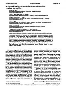
diagonal, matrix element, Hpy py is similar to Hpx px with x ←→ y and Hpy px = Hp∗x py . In this work we consider only these two bands. We have fitted the V and ε matrix elements for the E polarization case with cylinders of dielectric constant ǫ = 100 in vacuum, to the band structure of five different rectangular lattices with large/small axis ratios: 1, 1.05, 1.1, 1.15, 1.2 as well as to a hexagonal lattice, for six different filling ratios: f = .1, .2, .3, .4, .5, .6. We used a large value for the dielectric constant to ensure that we obtain large gaps and narrow bands. The quality of these fits can be seen in Fig. 1 where we plot the bands as found numerically by the plane wave expansion (PWE) method along with the TB fit, for a square and a hexagonal lattice for two filling ratios. The perfect quality of the fits is an indication of the potential usefulness of the TB method. We next plot some of the fitted matrix elements. The square root of the diagonal εpx and εpy matrix elements are plotted (Fig. 2a) as a function of the filling ratio f, while the off diagonal Vppπ matrix elements are plotted (Fig. 2c) as a function of the dimensionless separation distance dij = rij /α, where rij is the separation distance between cylinders i and j and α is the cylinders’ radius. Notice how bad the scaling is, especially for the Vppπ element. Apparently, a satisfactory TB description can not be achieved with this two-center approach, but rather, with the inclusion of the lattice environment [9] as well. The proposed simple rescaling function (Dnon )i for the diagonal matrix element that describes the lattice environment of cylinder i, and takes into account the filling ratio and the different symmetries is of the form:

~ R

where we have neglected crossing terms between the plane wave and the resonances (this is not completely justifiable, but it can be argued that they are not important for frequencies close to the gap, and so for impuR rity and disorder studies). β00 = Ψ∗0 (~r)HΨ0 (~r)d~r and R ~ = Ψ∗0 (~r)HΨ0 (~r − R)d~ ~ r , and hǫi is the averaged γ00 (R) dielectric constant. We argue that the functional form of |c20 (k)|2 is similar to the form of the scattering cross section of a single cylinder for the n = 0 (or s-wave) p case, 1 2 −λ(f )ωrµ ~ so that |c0 (k)| ≃ e . Here ωr = |k|c/(ω0 hǫi), ω0 is the single cylinder Mie resonance frequency, λ(f ) is a function of the filling ratio f of the form λ(f ) = b1 /f b2 . The power µ has to be larger than 2 in order to preserve the correct slope at |~k| → 0. For simplicity, we choose µ = 4. The second band (n = 1 or p-like) has a Ψ ∼ cos θ symmetry, and will consist of two linearly independent polarizations, px and py . There will be crossing terms between these two polarizations, but not between s-like and p-like resonances. Using the standard notation [6–8] for the matrix elements, and taking into account only first and second nearest neighbors, then the nonzero Hamiltonian matrix elements for the case of a square lattice with lattice constant a is: (1) Hss = |c10 |2 |k|2 /hǫi + |c20 |2 [εs + 2Vssσ ×

(2) ×(cos φx + cos φy ) + 4Vssσ cos φx cos φy ] (1) 2Vppπ

X τ cos2 (nθij ) 1 = on (Dn )i dνijn

where θij is the angle between the symmetry axis of the p resonance on cylinder i and the rˆij direction, n=0,1,.. for the s,p,.. resonances, and the sum runs over the nearest neighbors of cylinder i. The power on the angular function was chosen so that the px and py resonances in the hexagonal lattice be the same. The only choices were 2 and 4, and it was found that 2 gives better results. Eq. 6 is similar to what was used in Ref. [9] for the atomic orbitals, except for two differences: (a) here we take into account the resonance’s angular symmetry, and (b) the exponentially decaying part is missing, reflecting the non-localized character of the EM resonances. Fi 2 nally, τ = π/(a2 f ) is a renormalization that takes into account that different structures, with the same lattice constant a and cylinder radius α, have different filling ratios. τ is normalized so that τ = 1 for the rectangular structures and τ = 3/4 for the hexagonal. We will use this parameter only for the diagonal matrix elements. For the periodic case, the function (Dnon )i is the same for every i, and will characterize the corresponding resonance. We find the diagonal matrixn element to scale as n √ ǫn = an0 +an1 (Dnon )−a2 +an3 (Dnon )−a4 where an0 = ω0 α/c

(3)

(1) 2Vppσ

cos φy + cos φx + Hpx px = εpx +   (2) (2) cos φx cos φy +2 Vppσ + Vppπ   (2) (2) sin φx sin φy − Vppσ Hpx py = 2 Vppπ where φx = kx a, φy = ky a and |k| =

(6)

j6=i

(4) (5)

q kx2 + ky2 . V (1) ,

V (2) refer to the γ matrix elements for first and second nearest neighbors respectively, ε refers to the β, on-site or 2

b1 b2 b3 c1 c2 c3 Vssσ 0.075 0.0008 10.0 -0.108 4.00 -0.00096 Vppσ 0.100 0.00008 13.5 0.425 6.14 0.0550 Vppπ 0.700 0.0015 10.0 -0.076 5.40 -0.0044

is the corresponding dimensionless Mie resonance fre√ quency. In Fig. 2b we plot εp vs the environment √ function (1/Dpon ). We can see that εp now scales very well, having a larger value for increasing lattice density. The same dependence is found for all bands. In order to rescale the off diagonal V matrix element between two neighboring resonances i and j, we need contributions from the neighbors that are close to the line joining i and j. Contributions have to be projected on the rˆij direction for the s resonance, while for the p resonance we have to project on its symmetry axis. Only first nearest neighbors will contribute. At the end, we have to normalize with the sum of all projection weights. A simple formula that describes the environment of the n resonance on cylinder i, along the rˆij direction is: P νn 2 n 1 l (cos θilj /dil ) P (7) = 2 n (Dnof f )ij l cos θilj

c4 1.30 3.22 2.32

Next, we test our results on a nonperiodic lattice. The original periodic lattice is square with filling ratio f = 0.2 and lattice constant a. We will solve the 3×3 supercell problem. Each supercell consists of 9 cylinders, and the whole lattice is periodic in terms of this supercell. We keep all cylinders in the supercell in place, except the middle one, which we move from it’s periodic position (0, 0), a/4 towards the left, then a/4 towards the bottom, and then return to the periodic position (0, 0) along the diagonal (see insert graph in Fig. 3). Solving the supercell TB problem involves a 9×9 matrix diagonalization for the s band, and a 18×18 matrix diagonalization for the p band. We plot the 3 highest eigenvalues of the s band, and the 3 highest and 3 lowest eigenvalues of the p band. Luckily, for the 3 highest eigenfrequencies of the s band, we do not need to take into account the free plane wave, since for those frequencies the resonances are fully excited, blocking the background propagation mode. We plot the eigenfrequencies for ~ka = (0, 1/3), and directly compare our results with the ones obtained numerically by the PWE method, for the same exactly system. It is worth noting that in the PWE method, 100 plane waves per rod are needed for an acceptable numerical convergence. This is a factor of 104 more CPU time than the TB method. The agreement is excellent, so our TB parameterization works very well for the impurity case too. The photonic TB model proves to be an excellent tool for understanding and describing the band structure and properties of light in PBG structures. We hope that the calculated TB parameters will be used in studies of 2D PBG materials and can stimulate enough interest to extend these studies in 3D photonic crystals. We would like to thank C. Z. Wang and K. M. Ho for useful discussions. Ames Laboratory is operated for the U.S. Department of Energy by Iowa State University under Contract No. W-7405-Eng-82. This work was supported by the Director for Energy Research office of Basic Energy Sciences and Advanced Energy Projects, by NATO Grant No. 940647, and by a ΠENE∆ grant.

n where l runs over i’s nearest neighbors (including j). θilj is the angle between the rˆil and rˆij directions for the s resonance (n = 0), and for the p resonance (n = 1), it is the angle between the i’th resonance’s symmetry axis and the rˆil direction . Both angles are taken to have a range from −π/2 to π/2 [10]. Finally, if we include screening in our considerations, then the actual matrix element V to be used in a particular problem, can be obtained by the fully rescaled one V, by of f −1 V ij = V ij (1 − S ij )/[(Dof f )−1 )ji ] where S ij ij + (D ij is the same screening function used  in Ref. [9]: S = P b3 tanh b1 l6=i,j e−b2 [(dil +djl )/dij ] , and is different for different matrix elements. The fully rescaled matrix elements are found to scale with separation distance as 4 2 + c3 d−c V ij = c1 d−c ij . In Fig. 2d we plot the rescaled ij V ppπ matrix element. We see now that it is a smouth function of separation distance, except for the second nearest matrix elements which do not scale very well for large filling ratios (small distances). Apparently a screening function that depends on the filling ratio as well is needed, but for simplicity and to keep some accordance with the electronic models used so far, we will use this one. We find that all matrix elements now scale very well with separation distance, so a satisfactory TB description of PBG materials is in order. The rescaling parameters used and the parameters for the rescaled matrix element curves’ generation are presented in Tables 1 and 2. We have also found νn = 1.65 for all n, and b1 = .068, b2 = 1.23 for λ(f ).

TABLE I. The parameters for the ε elements. a0 a1 a2 a3 a4 √ εs 0.0804 0.0460 0.716 -0.0121 5.000 √ εp 0.2371 0.0890 1.640 0.0020 0.320

[1] a) See for example, Photonic Band Gaps and Localization, edited by C. M. Soukoulis (Plenum, New York, 1993); b) J. Opt. Soc. Am. B 10, 208-408 (1993); c) Photonic Band Gap Materials, edited by C. M. Soukoulis (Kluwer, Dordrecht, 1996). [2] J. Joannopoulos, R. D. Meade and J. Winn, Photonic Crystals, (Princeton University, Princeton, N. J. 1995).

TABLE II. The parameters for the V elements.

3

[3] S. Datta, C. T. Chan, K. M. Ho, C. M. Soukoulis and E. N. Economou in Ref. 1a p. 289. [4] M. Kafesaki, E. N. Economou and M. M. Sigalas in Ref. 1c p. 143. [5] G. Mie, Ann. Phys. 25, 377 (1908); C. F. Bohren and D. R. Huffman, Absorption and Scattering of Light by Small Particles (J. Wiley, New York, 1983, ch. 4). [6] J. C. Slater and G. F. Koster, Phys. Rev. 94, 1498 (1954). [7] D. A. Papaconstantopoulos, Handbook of the Electronic Structure of Elemental Solids, (Plenum Press, New York, 1986). [8] W. A. Harrison, Electronic Structure and the Properties of Solids, (Freeman, San Francisco, 1980). [9] M. S. Tang, C. Z. Wang, C. T. Chan, and K. M. Ho, Phys. Rev. B 53, 979 (1996). [10] Note however, that for Vppπ matrix elements, since both 1 lobes of the p resonance are involved, θilj must take all possible values, but we will have to average over the contributions to each lobe. Also note, that for the nonperiodic case, certain Hpx py and Hpy px matrix elements will not be complex conjugates if the formula is applied explicitly. In this event we have to average over the two possibilities, in order to keep the Hamiltonian matrix Hermitian. FIG. 1. The first two frequency bands for a square lattice with filling ratio f = .1 (a) and f = .4 (b), and for a hexagonal lattice with f = .1 (c) and f = .4 (d). Circles correspond to numerical results from the PWE method, while solid lines correspond to the TB fit.

FIG. 2. Fitted TB parameters for the second (p-like) fre√ √ quency band. (a) εp vs f . (b) εp vs the rescaled envion ronment function 1/Dp . Circles and squares correspond to √ √ εpx and εpy respectively of a rectangular lattice with the big axis along x ˆ, and triangles to a hexagonal lattice. (c) Vppπ vs the separation d. (d) The rescaled V ppπ vs d. Circles, squares and diamonds correspond to a rectangular lattice’s Vppπ elements along the small axis, the large axis and the diagonal, and triangles to a hexagonal lattice. All matrix elements are expressed in the dimensionless units of (ωα/c)2 .

FIG. 3. The three edge eigenfrequencies for each band for a 3 × 3 impurity system. All cylinders are identical, with the midlle one moving from the equilibrium position, as pointed in the insert graph. The wave vector is always constant ~ka = (0, 1/3). The first band gap extends approximately from ωa/c ≃ .53 to ωa/c ≃ .87, while the second starts at ωa/c ≃ 1.03

4

1.00

1.5

0.75

1.0

0.50

0.5

0.25

(a)

ωa/c

0.0

Γ

(b) Μ

X

Γ

0.00

Γ

X

Μ

Γ

Μ

Γ

1.00

1.5

0.75

1.0

0.50

0.5

0.25

(d)

(c) 0.0

Γ

X

Μ

Γ

0.00

Γ

X

Lidorikis et al. Figure 1

0.28

0.28

(a)

√εp

0.27

|

0.26

0.26

0.25

0.25

0.24

0.24 0.2

0.4

0.6

0.2

f

×10

-2

0.0

(b)

0.27

0.4

1/Dp

×10

-2

0.0

0.6

on

Vppπ

-0.1 -0.1

-0.2 -0.3

-0.2

-0.4 -0.5

(c) 2

4

6

d

(d) 8

-0.3

2

4

6

d

Lidorikis et al. Figure 2

8

1.05

0.95

ωa/c

0.85

0.75

a 0.65

0.55

0.45 (0,0)

(-a/4,0)

(-a/4,-a/4)

(0,0)

Impurity Position

Lidorikis et al. Figure 3