Tightening simple mixed-integer sets with guaranteed bounds. Daniel Bienstock and Benjamin McClosky. Columbia University. New York. July 2008. Abstract.
Tightening simple mixed-integer sets with guaranteed bounds Daniel Bienstock and Benjamin McClosky Columbia University New York July 2008 Abstract In this paper we study how to reformulate knapsack sets and simple mixed integer sets in order to obtain provably tight, polynomially large formulations.
1
Introduction
In this paper we consider 0/1 knapsack sets and certain simple fixed-charge network flow sets. The study of such sets is relevant in that a popular approach for solving general mixed-integer programs consists of selecting a subset of constraints with particular structure (such as a single-node fixedcharge flow problem) and tightening that part of the formulation through the use, for example, of classical cutting-plane families (see e.g. [14], [11]). A question of interest is in what sense the resulting stronger formulation is provably good. Motivated by questions posed in [17], and extending the study initiated in [3], we show how the use of appropriate disjunctions [1] leads to provably tight, yet polynomially large, formulations for several simple sets. Unlike the use of familiar disjunctive cuts ([2], [16] and [9], [10]) the disjunctions we employ are ‘combinatorial’, or ’structural’, that is to say, they depend on the structure of the problem at hand. Previous work [6] has shown how structural disjunctions can lead to provably good approximations of combinatorial polyhedra (also see [12], [4], [5]); we expect that many other results of this type are possible. 1.0.1
Minimum knapsack
In Section 2 we consider the “minimum” 0/1 knapsack problem,
(KMIN ) :
vZ
= min
N X
cj xj ,
j=1
s.t.
N X
j=1
wj xj ≥ b,
x ∈ {0 , 1}N ,
(1) (2)
where cj > 0 and 0 < wj ≤ b for 1 ≤ j ≤ N . We denote by v ∗ the value of the LP relaxation of KMIN . In [8], Carr, Fleischer, Leung and Phillips consider the so-called knapsack-cover inequalities, which P are different from cover inequalities. Given a set A ⊆ {1, . . . , N } write b(A) = b − j∈A wj . Then the knapsack-cover inequality corresponding to A is X
j ∈A /
min{wj , b(A)}xj ≥ b(A). 1
In [8] it is shown that the relaxation to KMIN provided by all knapsack-covers yields a lower bound vˆ to v Z such that v Z ≤ 2ˆ v . On the other hand, the price to be paid is that the algorithm used to (approximately) solve this relaxation is fairly complex – a separation procedure for knapsack-covers is not given. We show how a simple disjunction provides a polynomially large linear programming relaxation to KMIN whose value v¯ satisfies v Z < 2¯ v . In fact, we show Theorem 1.1 For� each 0 < � < 1 there is a linear programming relaxation to KMIN with � 2) O(1/� O (1/�) N 2 variables and constraints, whose value v(�) satisfies v Z < (1 + �)v(�).
Recently, Carnes and Shmoys [7] presented a primal-dual, 2-approximation algorithm for KMIN that relies on knapsack-cover inequalities. The constructions underlying Theorem 1.1 can be used to tighten the approximation factor in [7] to (1 + �) for arbitrary 0 < � < 1; as far as we know, this is the first such result for KMIN . 1.0.2
Fixed-charge sets
In Section 3 we consider the fixed-charge network flow problem. We consider the following generalization given by the following mixed-integer program: (FX N ) :
vZ
= min
X
(fij yij + cij xij ) ,
(i,j)∈A
X
(i,j)∈δ + (i)
xij −
0 ≤ xij ≤ uij yij yij = 0 or 1,
X
xji = bi ,
(j,i)∈δ − (i)
∀i ∈ I,
∀(i, j) ∈ A,
∀(i, j) ∈ A.
(3) (4) (5)
Here, • We are given a directed graph G, • A is the set of arcs; for each (i, j) ∈ A we have c ij , fij nonnegative and uij > 0, • The vertex set of G is partitioned into two classes: I (the “inner” vertices) and O (the “outer” vertices), • For each i ∈ I there is a real bi ; δ + (i) (resp., δ − (i)) is the set of arcs of the form (i, j) (resp., (j, i)), • Each vertex v ∈ O is incident with a unique arc; the other endpoint of that arc is an inner vertex. In this paper we consider the special case of this problem where the inner vertices induce a path; see Figure 1. In this case we have a generalization of the single-item lot-sizing problem. The following result holds: Theorem 1.2 Assuming I�induces a path, then for each � 0 < � < 1 there is a linear programming 2) O(1/� 3 3 relaxation to FX N with O (1/�) (1 + |O|) |I| variables and constraints, whose value v(�) satisfies v Z < (1 + �)v(�).
2
= inner
= outer
Figure 1: Fixed-charge set. Carnes and Shmoys [7] also present a 2-approximation algorithm for the single-item lot-sizing problem; our constructions can be used to tighten their results to obtain 1 + �-approximation algorithms. 1.0.3
Maximum knapsack
In Section 4 we consider the “maximum” 0/1 knapsack problem, (KMAX ) :
v
Z
= max
N X
pj xj ,
j=1
s.t.
N X
j=1
wj xj ≤ b,
x ∈ {0 , 1}N ,
(6) (7)
where pj > 0 and 0 < wj ≤ b for 1 ≤ j ≤ N . We denote by v ∗ the value of the LP relaxation of KMAX . In [17] Van Vyve and Wolsey ask whether, given an instance of KMAX , and 0 < � ≤ 1, there is a formulation of the form Ax + A0 x0 ≤ b0 , such that (a) For each vector x ∈ {0 , 1}n with
Pn
j=1 wj xj
≤ b there exists x0 such that Ax + A0 x0 ≤ b0 ,
(b) The number of variables x0 and rows of A and A0 is polynomial in n and/or �−1 , and n, (c) For every w ∈ R+
n
max wT x : Ax + A0 x0 ≤ b0
o
≤ (1 + �)v Z .
In [3] we provided a partial answer to this question: there is a formulation satisfying (a)-(c) which has polynomially many variables and constraints for each fixed �. This formulation amounts to a multi-term disjunction, which, although polynomial, is complex from a practical perspective. The result in [3] motivates several questions, in particular: 1. Is there a formulation achieving (a)-(c) but restricted to the original space of variables? 2. How about achieving (c), but restricting to the original space of variables and allowing exponentially many constraints, so long as these are polynomially separable? 3
3. In fact, what can be achieved in polynomial time? Assuming w j ≤ b for all j, it is known that v ∗ /v Z < 2, and that this bound is best possible. Is there a “simple” relaxation involving polynomially separable inequalities, whose value vˆ satisfies vˆ/v Z < θ for some θ < 2? Concerning (a), a natural question to ask is the following. Suppose we pick a fixed integer k > 0, P and we strengthen the LP relaxation of KMAX with all valid inequalities of the form j αj xj ≤ β, where the αj take values in {0, 1, . . . , k}. Is it true that the value of the resulting linear program is at most (1 + f (1/k))v Z , where f (�) → 0 as � → 0? The answer to this question is (perhaps, not surprisingly) negative. We show that for each k > 0, if N is large enough there is an example of KMAX where, after adding all valid inequalities with left-hand coefficients in {0, 1, . . . , k}, the value of linear program remains arbitrarily close to 2v Z . This is discussed in Section 4.1. Thus, valid inequalities with “small” coefficients are not enough to get an LP to IP ratio strictly bounded away from 2. At the same time, in Section 4.2 we show that using a �(polynomially separable) disjunction, one obtains � √ 19−2 v Z . Thus, question 3 above does have a positive a relaxation whose value is at most 1 + 3 answer. However, the disjunction used in Section 4.2 depends on the structure of the objective coefficients pj and is therefore not quite in the “a priori strengthening” spirit of the question of Van Vyve and Wolsey. Further, the examples in Section 4.1 have “large” constraint coefficients, that is to say we have wj ≈ b for some j. One might consider such examples “artificial” and wonder what happens when they are excluded. These issues are taken up in Section 4.3. Given a subset S ⊆ {1, 2, . . . , N } with w i + wj > b for each pair of distinct indices i, j ∈ S, the clique inequality [13] X
j∈S
xj ≤ 1
is valid for KMAX . Let v ω denote the value of the linear program obtained by augmenting the continuous relaxation of KMAX with all clique inequalities. In Section 4.3 we prove: Theorem 1.3 For each constant 0 ≤ λ < 1 there exists � = �(λ) > 0 satisfying the following property. For N large enough, if wj ≤ λb for 1 ≤ j ≤ N , then v ω ≤ (2 − �)v Z .
2
Minimum knapsack problem
In this section we consider problem KMIN and prove Theorem 1.1. Our construction is inspired by that in [18], [5] in the context of the set-covering problem, and it relies on disjunctive inequalities. Prior to our main proof, we will first show a simpler result in order to motivate our approach. In what follows we will assume without loss of generality that c1 ≥ c 2 ≥ . . . ≥ c N .
(8)
For 1 ≤ h ≤ N , let P h denote the polyhedron defined by: N X
j=1
wj xj ≥ b,
(9)
x1 = x2 = · · · = xh−1 = 0, xh = 1, 0 ≤ xj ≤ 1, h < j ≤ N. 4
(10) (11)
and write M
�
�
= conv P 1 ∪ P 2 ∪ · · · P N , n
o
v¯ = min cT x : x ∈ M .
(12) (13)
Note that M is the projection to RN of the feasible set for a system of O(N 2 ) linear constraints in O(N 2 ) variables. We have that x ∈ M for any 0/1 vector x that satisfies (9) and therefore v¯ ≤ v Z . Lemma 2.1 v Z < 2¯ v. Proof. Let x ¯ be a solution to the linear program (13). It follows that there reals λ h such that 0 ≤ λh , (1 ≤ h ≤ N ),
N X
λh = 1,
h=1
and, for each 1 ≤ h ≤ N with λh > 0, a vector xh ∈ P h , such that x ¯ =
X
λh xh .
h : λh >0
For 1 ≤ h ≤ N write o
n
v h = min cT x : x ∈ P h .
(14)
Suppose λh > 0. It is straightforward to see that there is an optimal solution to (14) with at most one fractional variable. By rounding up this variable we obtain a feasible 0/1 solution to the original knapsack problem. We therefore have by (8) and (10) v Z − v h < c h ≤ c T xh ,
(15)
where the second inequality follows since x hh = 1 again by (32). Consequently, writing Λ = {1 ≤ h ≤ n : λh > 0} , we have v Z − v¯ = ≤ =
X
λh v Z −
X
λh v Z −
X
λh v Z − v h
X
λh cT xh = v¯.
h∈Λ
h∈Λ
h∈Λ
1.] For each 1 ≤ h ≤ N , and each signature σ, define P h,σ = { x ∈ [0, 1]N :
N X
j=1
wj xj ≥ b,
(31)
x1 = x2 = · · · = xh−1 = 0, xh = 1, X
xj = σ k ,
X
xj ≥ J,
j∈S h,k
j∈S h,k
}.
∀k such that σk < J, ∀k such that σk = J
(32) (33) (34)
Lemma 2.4 ˆ h,σ feasible for KMINo such that cT x ˆh,σ ≤ o σ there is a 0/1 vector x n n For each h and (1 + �) min cT x : x ∈ P h,σ . As a result, v Z ≤ (1 + �) min cT x : x ∈ P h,σ . Proof. Let x ¯ ∈ P h,σ . We x ˆh,σ as follows. First, for each k such that σ k > 0, we obtain the values h,σ h,k by applying Lemma 2.2 with S = S h,k . Here, note that when σk < J, the we x ˆj for each j ∈ S have cmax cmax 1 ≤ min ≤ 1 + �, + 1− min σk σk c c 7
by construction of the sets S h,k . And if σk = J, we also have �
1+
cmax J cmin
�
≤ 1 + �,
(35)
by our choice for J. If on the other hand σ k = 0 we set x ˆh,σ = 0 for every j ∈ S h,k . j Finally, define T h = {j : cj ≤ (1 + �)−K }. The problem min
X
cj xj
X
wj xj ≥
(36)
j∈T h
s.t.
j∈T h
0 ≤ xj ≤ 1,
X
wj x ¯j
(37)
∀ j ∈ T h,
(38)
j∈T h
is a knapsack problem, and hence it has an optimal solution x ˜ with at most one fractional variable. h ; thereby increasing cost (from x We set x ˆh,σ = d˜ x e for each j ∈ T ˜) by less than (1+�) −K ch ≤ � ch j j by definition of K. In summary, cT x ˆh,σ − cT x ¯ =
X
k : σk >0
≤ �
X
X
cj x ˆh,σ j −
X
cj x ¯ j + � ch
j∈S h,k
X
j∈S h,k
cj x ¯j +
X
j∈T h
cj (ˆ xh,σ ¯j ) j −x
(39) (40)
k : σk >0 j∈S h,k
≤ � cT x ¯.
(41)
Here, (40) follows from Lemma 2.2, and by definition of the sets S h,k , and (41) follows from the fact that x ¯h = 1, by definition of P h,σ . Consider the polyhedron
Q = conv
[
h,σ
�
P h,σ . 2
(42)
�
Note that there are at most (J + 1)K N = O (1/�)O(1/� ) N polyhedra P h,σ , and that each P h,σ is described by a system with O(K + N ) constraints in N variables. Thus, Q is the projection to RN of the feasible set for a system with at most O
� �O(1/�2 )
1 �
N
2
!
constraints in O
� �1/� !
1 �
N 2 variables.
(43)
Furthermore, any 0/1 vector x that is feasible for the knapsack problem satisfies x ∈ P hσ for some h and σ; in other words, Q constitutes a valid relaxation to the knapsack problem. Lemma 2.5 v Z ≤ (1 + �) min{cT x : x ∈ Q}. 8
Proof. Let x ˜ ∈ Q. Then there exist reals λ h,σ , for each 1 ≤ h ≤ N and σ ⊆ {1, 2, . . . , K}, such that 0 ≤ λh,σ , ∀ h and σ,
and
XX h
λh,σ = 1,
σ
and, for each h and σ with λh,σ > 0, a vector xh,σ ∈ P h,σ , such that x ˜ =
λh,σ xh,σ .
X
h,σ : λh,σ >0
Let Λ = {(h, σ) : λh,σ > 0}. Then v Z − cT x ˜ = =
X
λh,σ v Z −
X
λh,σ
X
λh,σ � cT xh,σ
(h,σ)∈Λ
(h,σ)∈Λ
≤
(h,σ)∈Λ
�
X
λh,σ cT xh,σ
v Z − cT xh,σ
�
(44)
(h,σ)∈Λ
�
�
(by Lemma 2.4)
= � cT x ˜,
(45) (46) (47)
as desired. Note that the proofs above rely on term-by-term rounding of a solution to a linear program. As a consequence, we have the following result, whose proof we include for completeness, though it essentially follows from Lemmas 2.4 and 2.5. Corollary 2.6 For each 0 < � < 1 there is an algorithm that computes a feasible 0/1 solution to Z the minimum-knapsack � � problem, with value at most (1 + �)v . This algorithm requires the solution 2 of O (1/�)O(1/� ) N linear programs with O(N ) variables and constraints.
Proof. By Lemma 2.4, for each h and σ there is a 0/1 ˆ h,σ which is feasible for the n vector x o T h,σ T h,σ knapsack problem, and such that c x ˆ ≤ (1 + �) min c x : x ∈ P . From among the set
Z T Z ≤ of all vectors ˆh,σ select one o of minimum cost; denoting this vector by x wenhave c x o n x (1 + �) min cT x : x ∈ P h,σ for each h and σ, and as a result cT xZ ≤ (1 + �) min cT x : x ∈ Q .
3
Fixed-charge network flow problems
In this section we consider the mixed-integer programs FX N described in the introduction, in the case where the inner vertices I induce a path. In order to motivate the discussion we first discuss some special cases.
3.1
Single inner node
Let I = {1}; we then have A = δ + (1) ∪ δ − (1). To simplify notation we will index the arcs by the integers 1, 2, . . . , n = |A|. We assume that the arcs have been numbered so that fk + ck uk ≥ fk+1 + ck+1 uk+1 , for 1 ≤ k < n. 9
Problem FX N can be written as vZ
= min
n X
(fj yj + cj xj ) ,
(48)
j=1
X
j ∈ δ + (1)
X
xj −
0 ≤ x j ≤ u j yj yj = 0 or 1,
xj
= b1 ,
(49)
j ∈ δ − (1)
∀j,
(50)
∀j.
(51)
Given a vector (x, y) feasible for FX N an arc j is called slack if y j = 1 and 0 < xj < uj yj . Otherwise the arc is called tight. The following result is routine. Lemma 3.1 In any extreme point solution to (48)-(51) there is at most one slack arc. 3.1.1
Achieving a bound of 2
For each pair of indices 1 ≤ h, i ≤ n (including i = h), consider the polyhedron D h,i defined by j
X
∈ δ + (1)
xj −
j
X
xj
= b1 ;
∈ δ − (1)
0 ≤ yj ≤ 1 ∀ j ∈ A,
(52)
yi = yh = 1; if h 6= i then yg = 0 ∀ g 6= i with g < h;
(53)
0 ≤ x i ≤ u i yi ;
(55)
if h = i then yg = 0 ∀ g 6= h, x g = u g yg
∀ g 6= i.
(54)
Now as a consequence of Lemma 3.2 we have: Lemma 3.2 Let (ˆ x, yˆ) 6= (0, 0) be an extreme point solution to (48)-(51). Then there exist indices 1 ≤ h, i ≤ n such that (ˆ x, yˆ) ∈ D h,i . Proof. We have yˆ 6= 0. If there is a unique index j with yˆj = 1, then set i = h = j and we are done. Otherwise, (using Lemma 3.1) let h be the minimum index j with yˆj = 1 and x ˆj = uj yj . Again using Lemma 3.1 there is at most one index j with yˆj = 1 and 0 < x ˆj < uj ; we set i equal to that index if it exists, and we set i = h otherwise. Define:
Q =
� �S h,i h,i D conv
if b1 6= 0,
� � conv (0, 0) ∪ S D h,i otherwise. h,i
As a consequence of Lemma 3.1 we have that if (ˆ x, yˆ) is feasible for (48)-(51) then (ˆ x, yˆ) ∈ Q. Lemma 3.3 For each pair of indices 1 ≤ h, i ≤ n, v Z ≤ 2 min{cT x + f T y : (x, y) ∈ D h,i }.
10
n
o
Proof. Let (¯ x, y¯) be an optimal extreme point solution to min cT x + f T y : (x, y) ∈ D h,i , and assume by contradiction that there exist indices p 6= q with 0 < y¯p < 1 and 0 < y¯q < 1. Then p, q 6= h and p, q 6= i. Consequently, x ¯ p = up y¯p and x ¯q = uq y¯q , and therefore x ¯p > 0 and x ¯q > 0. + + Assume first that p ∈ δ (1) and q ∈ δ (1). Then for real δ small enough in absolute value, we can reset yp ← y¯p + δ, xp ← x ¯p + up δ, up δ, xq ← x ¯q − up δ, yq ← y¯q − uq
(56) (57)
maintaining feasibility for D h,i , contradicting the assumption that (¯ x, y¯) is an extreme point. The remaining cases (both p and q in δ − (1), one each in δ + (1) and δ − (1)) are similarly handled. Thus, there is a unique index i with 0 < y¯g < 1. Setting yg = 1 (and keeping all other variables unchanged) yields a feasible solution to FX N ; since g > h and all costs are nonnegative this change at most doubles the cost. As a corollary we now have v Z ≤ 2 min{cT x + f T y : (x, y) ∈ Q}. 3.1.2
Achieving a bound of 1 + �
Let 0 < � < 1. In order to improve the IP/LP ratio from 2 to 1 + �, we apply the technique used in Section 2.1 to prove the corresponding result for the minimum knapsack problem. In the context of the single inner-node problem, this works out as follows: rather than constructing a disjunction based on the polyhedra D h,i as defined above, instead we construct a disjunction using polyhedra D h,i,σ , where σ is a signature (see Definition 2.3). The polyhedra D h,i,σ are obtained by adapting the definition of D h,i given above, in particular, equation (54), in order to mirror equations (33), (34). The proof that the resulting disjunction proves the desired 1 + � bound is much like the proof of Lemmas 2.4, 3.3.
3.2
Two inner nodes
We assume I consists of nodes 1 and 2, and that the arc between 1 and 2 is (1, 2). For i = 1, 2, write ∆(i) = δ − (i) ∪ δ + (i) \ (1, 2). The following result is straightforward. Lemma 3.4 In an optimal solution to (x, y) for FX N , without loss of generality either (a) y12 = 1 and x12 = u12 , or y12 = 0 and x12 = 0; and in either case there is at most one slack arc in ∆(1) and at most one slack arc in ∆(2). (b) y1 = 1 and 0 < x1 < u1 ; and there is at most one slack arc in ∆(1) ∪ ∆(2). We now show how to generate a polynomial-size relaxation that yields an IP/LP ratio of at most 2. Using Lemma 3.4 it is straightforward to do so with a disjunction with O(n 4 ) terms relying on the results of the previous section. However, we will show how achieve the same bound with O(n 2 ) terms using a system of nested disjunctions. We number the arcs in ∆(1) ∪ ∆(2) as 1, 2, . . . , n − 1, where the indices reflect non-increasing values of fj + cj uj (we will still refer to the arc between 1 and 2 as (1, 2), however).
11
∆(1)
h,i Let h, i ∈ ∆(1). For φ = 0 or φ = 1, consider the polyhedron D 1,φ ⊆ R+ by:
X
j ∈ δ + (1)\(1,2)
xj −
X
j ∈ δ − (1)
xj − (b1 − u12 φ) α = 0,
∆(1)
× R+
× R+ defined
0 ≤ yj ≤ α, ∀ j ∈ ∆(1)
yh = yi = α; if h 6= i then yg = 0 ∀ g ∈ ∆(1) with g 6= i and g < h; if h = i then yg = 0 ∀ g ∈ ∆(1) \ h,
0 ≤ x i ≤ u i yi ; x g = u g yg 0 ≤ α.
∀ g 6= i with g ∈ ∆(1),
(58)
(59) (60) (61)
Note: The quantity α is a homogenization factor, the user should think of it as taking values either 1 or 0 (in the latter case all x and y will take value zero). Also, when φ = 1 (resp., 0) (58) corresponds to the flow conservation constraint at node 1 assuming the arc (1, 2) carries flow u 12 (resp., 0), both after homogenization. h,i Similarly, for each pair h, i ∈ ∆(2), and φ = 0 or φ = 1, consider the polyhedron D 2,φ ⊆ ∆(2)
R+
∆(2)
× R+
× R+ defined by:
X
j ∈ δ + (2)
xj −
X
j ∈ δ − (2)\(1,2)
xj − (b2 + u12 φ) β = 0,
0 ≤ yj ≤ β, ∀ j ∈ ∆(2)
yh = yi = β; if h 6= i then yg = 0 ∀ g ∈ ∆(2) with g 6= i and g < h; if h = i then yg = 0 ∀ g ∈ ∆(2) \ h,
0 ≤ x i ≤ u i yi ; x g = u g yg 0 ≤ β.
∀ g 6= i with g ∈ ∆(2),
(62)
(63) (64) (65)
Finally, writing ∆ = ∆(1) ∪ ∆(2), then for each pair of indices h, i ∈ ∆ consider the polyhedron T h,i defined by:
j
X
∈ δ + (1)\(1,2)
xj −
j
X
∈ δ − (1)
xj − b1 γ = 0,
j
X
∈ δ + (2)
xj −
j
X
∈ δ − (2)\(1,2)
xj − b2 γ = 0,
0 ≤ yj ≤ γ ∀ j ∈ ∆, y12 = γ,
0 ≤ x12 ≤ u12 y12 ,
(67)
yh = yi = γ; if h 6= i then yg = 0 ∀ g ∈ ∆ with g 6= i and g < h; 0 ≤ x i ≤ u i yi ;
if h = i then yg = 0 ∀ g ∈ ∆ \ h, x g = u g yg
(66)
∀ g 6= i.
(68) (69)
h,i Roughly speaking the Dk,δ polyhedra capture case (a) of Lemma 3.4 whereas the T h,i will be shown to capture case (b).
Our overall formulation can now be given. For k = 1, 2 we will use the notation (x(k), y(k)) to denote an (x, y) vector with entries for arcs in ∆(k). For convenience of notation, we will also assume that b1 6= 0 and b2 6= 0; we will indicate later how to handle the other cases as well. Using (somewhat abused) vector notation, the formulation is:
12
(x(1), y(1), x12 , y12 , x(2), y(2), 1) = X
X
(x(1)i,h,φ , y(1)i,h,φ , u12 φ αi,h,φ , φ αi,h,φ , x(2), y(2), αi,h,φ ) +
φ=0,1 i,h∈∆(1)
X
i,h (ˆ x(1)i,h , yˆ(1)i,h , x ˆi,h ˆ12 ,x ˆ(2)i,h , yˆ(2)i,h , γ i,h ) 12 , y
(70)
i,h∈∆ h,i (x(1)i,h,φ , y(1)i,h,φ , αi,h,φ ) ∈ D1,φ ,
∀ φ, and ∀ i, h ∈ ∆(1)
i,h (ˆ x(1)i,h , yˆ(1)i,h , x ˆi,h ˆ12 ,x ˆ(2)i,h , yˆ(2)i,h , γ i,h ) ∈ T h,i , 12 , y
(x(2), y(2), αi,h,φ ) =
X
X
0
0
0
(71)
∀ i, h ∈ ∆ 0
0
0
(72) 0
0
0
(x(2)i ,h ,φ , y(2)i ,h ,φ , β i ,h ,φ )
φ0 =0,1 i0 ,h0 ∈∆(2)
for all φ = 0, 1, and i, h ∈ ∆(1)
0 0
h ,i (x(2)i ,h ,φ , y(2)i ,h ,φ , β i ,h ,φ ) ∈ D2,φ 0 , 0
0
0
0
0
0
0
0
0
(73)
∀ φ0 = 0, 1, and i0 , h0 ∈ ∆(2).
(74)
Note that the vector equation (70) includes the condition φ=0,1 i,h∈∆(1) αi,h,φ + i,h∈∆ γ i,h = 1. Thus, (70) describes a disjunction. The second term in the right-hand side of (70) corresponds to case (b) of Lemma 3.4, whereas the first term corresponds to case (a) and we disjunct on the arcs of ∆(1) and whether y12 = 0 or 1. Moreover, for a given φ = 0, 1, and i, h ∈ ∆(1), (73) requires that P
αi,h,φ =
X
X
0
P
P
0
0
β i ,h ,φ .
φ0 =0,1 i0 ,h0 ∈∆(2)
Thus (73) is also a disjunction (more precisely: it is a disjunction when α i,h,φ > 0, after scaling the equation by 1/αi,h,φ ). Based on these observations it follows that (70)-(74) describes a valid relaxation for FX N . We can now present the rounding result. Lemma 3.5 v Z ≤ 2 min{cT x + f T y : (x, y) satisfies (70)-(74) }. Proof. Consider an extreme point optimal solution (x(1), y(1), x 12 , y12 , x(2), y(2)) to the relaxation with constraints (70)-(74) chosen in addition so that the sum of α i,h,φ is maximum. 0
0
0
0
0
0
0
0
0
Note first that for each φ0 = 0, 1, and i0 , h0 ∈ ∆(2) we can “round” (x(2)i ,h ,φ , y(2)i ,h ,φ , β i ,h ,φ ) h0 ,i0 i0 ,h0 ,φ0 for every (u, v) ∈ ∆(2), while at most to a vector feasible for D2,φ 0 such that yu,v = 0 or β doubling the cost. This is analogous to the proof of Lemma 3.3 in the single inner-node case. A similar observation applies for each φ = 0, 1, and i, h ∈ ∆(1) – the vector (x(1) i,h,φ , y(1)i,h,φ , αi,h,φ ) h,i can be rounded to a vector feasible for D 1,φ such that yu,v = 0 or αi,h,φ for every (u, v) ∈ ∆(1), while at most doubling the cost.
13
Thus, by (70), the proof of the Lemma will be complete if we can prove a similar rounding result i,h for each vector (ˆ x(1)i,h , yˆ(1)i,h , x ˆi,h ˆ12 , xˆ(2)i,h , yˆ(2)i,h , γ i,h ) where i, h ∈ ∆, and γ i,h > 0. 12 , y Following the proof of Lemma 3.3, this result would follow if we can show that there is at most one arc (u, v) ∈ ∆ such that 0 < yˆuv < γ i,h . In turn, this is clear if 0 < x ˆ 12 < γ i,h u12 . So assume i,h not. Then either 0 = x ˆ12 , or x ˆ12 = γ u12 . In the first case by nonnegativity of the costs we can assume without loss of generality that 0 = yˆ12 . But then in either case term (72) in the disjunction corresponding to (i, h) corresponds to an instance of case (a) (with φ = 0 and φ = 1, respectively). It follows that there is an equivalent representation of (x(1), y(1), x12 , y12 , x(2), y(2)) where the sum of αi,h,φ has been increased by γ i,h , a contradiction. Above we had assumed that b1 6= 0 and that b2 6= 0. If not, in order to make the construction complete we simply need to add terms to the disjunctions given above corresponding to solutions where all arcs in ∆(1) or ∆(2) are set at zero (zero flow and zero y variables). It is straightforward to show that Lemma 3.5 still holds, as the proof given above proceeded on a term-by-term basis.
3.3
General case
We only sketch the construction in the case that I induces a general path, which we denote by P. In this case one can obtain a result similar to Lemma 3.4. An extreme point solution (ˆ x, yˆ) to FX N (where by definition yˆ is a 0/1-vector) can be decomposed into intervals: we have P = P1 ∪ P2 ∪ . . . Pk , where 1. The Pi are vertex-disjoint supbaths of P. 2. For any arc j ∈ P, 0 < x ˆ j < uj if and only if both ends of j belong to the same subpath P i . The formulation of the relaxation is similar to that given by (70)-(74), with the difference that there are |I| − 1 nested levels of disjunctions. The building blocks of the disjunctions correspond to intervals; for each interval we need to specify indices i, h as above, as well as up to two values φ, φ0 , each corresponding to the condition (flow at zero or at upper bound) of each arc connecting the interval to the rest of P. As was the case for the minimum-knapsack problem, the constructions can be used to yield approximation algorithms: Corollary 3.6 Given an instance of FX N where the inner vertices induce a path, for each 0 < � < 1 there that computes a feasible 0/1 of cost at most (1 + �)v Z . This algorithm � � is an algorithm 2 solves O (1/�)O(1/� ) (1 + |O|)2 |I|2 linear programs in O(|O| + |I|) variables. There are several ways in which Theorem 1.2 and Corollary 3.6 can be generalized, always relying on the basic disjunctive technique given above. An open case is that where the inner nodes induce a graph of fixed tree-width (the fixed path-width case is an easy extension). See [15].
14
4
Maximum knapsack
In this section we will present the results on the maximum knapsack problem. First we will show that using valid inequalities with “small” coefficients then the LP/IP ratio can remain arbitrarily close to 2. Then we we will discuss our use of disjunctions, and finally we will provide our analysis of clique inequalities in the case that the coefficients w j are not “large”.
4.1
Valid inequalities with small coefficients
Consider the knapsack instance with N = n + 1 where p1 = p2 = . . . = pn = 1, pn+1 = n,
√ w1 = w2 = . . . = wn = 1, wn+1 = n2 − b nc,
b = n2 . √ Write s = b nc. Clearly,
v Z = n + s ∼ n.
The lifted cover inequality,
n X
j=1
xj + (n − s)xn+1 ≤ n
defines a facet of conv(KMAX ). This suggests that the set of valid inequalities with ’small’ coefficients may not adequately approximate conv(KMAX ), but it is not clear how large the shortfall is. Consider the valid inequalities with left-hand side coefficients 0 or 1, which are as follows: ∀ A ⊆ {1, 2, . . . , n}, ∀ A ⊆ {1, 2, . . . , n},
X
xj ≤ |A|, and
X
xj + xn+1 ≤
j∈A
j∈A
(
(75) |A| + 1, if |A| ≤ s, |A|, otherwise.
(76)
Let x∗ be the point defined by x∗j = 1 − 1/s, for 1 ≤ j ≤ n + 1. It is not difficult to show that x∗ satisfies all inequalities (76) as well as (6), for n large enough. At the same time, we have Pn+1 ∗ j=1 pj xj = n − s + n − n/s ∼ 2n. However, a stronger result can be proved. Lemma 4.1 Let 0 < � < 1. Consider the knapsack instance with N = n + 1 where p1 = p2 = . . . = pn = 1, pn+1 = n,
(77) 2
w1 = w2 = . . . = wn = 1, wn+1 = n − n/2, 2
b=n .
(78) (79)
Let n+1 X j=1
αj xj ≤ β
(80)
be a valid inequality for the knapsack polytope defined by (77)-(79), where α j ∈ {0, 1, . . . , bn1−� c} for 1 ≤ j ≤ n + 1. Consider the point x ˆ with x ˆ j = 1 − 2n−� for 1 ≤ j ≤ n + 1. Then for n large enough, x ˆ is feasible for the continuous relaxation of KMAX and satisfies (80). 15
Proof. The first assertion is clear. To prove the second, let B denote the sum of the n/2 largest α j chosen among the indices 1 ≤ j ≤ n. Then, without loss of generality, β = max
n X
αj , B + αn+1
.
j=1
Consider first the case where there are at least n/2 positive α j with 1 ≤ j ≤ n. Then n+1 X j=1 n X
j=1
αj x ˆj
(1 + r)v Z . Since wj ≤ b for each j, we have that pj < 2/(1 + r) for each j. Define Ω = {j : pj ≥ r} , and w ˜ = min{wj : j ∈ Ω}. Let j ∗ ∈ Ω be such that wj ∗ = w ˜ (if Ω = ∅ j ∗ will be irrelevant). We have that KMAX
⊆ conv( L2 ∪ L1 ∪ L0 ),
(83)
where Li , 0 ≤ i ≤ 2 are the following convex polyhedra. First, L 2 is the set of solutions to the system: N X
wj xj ≤ b,
(84)
xj ≥ 2,
(85)
0 ≤ xj ≤ 1, ∀ j.
(86)
j=1
X
j∈Ω
Similarly, L1 is the set of solutions to the system: N X
j=1
X
wj xj ≤ b,
(87)
xj = 1,
(88)
j∈Ω
xj = 0, ∀ j 6= j ∗ with wj + w ˜ > b, 0 ≤ xj ≤ 1, ∀ j.
16
(89) (90)
Finally, L0 is the set of solutions to the system: N X
wj xj ≤ b,
(91)
xj = 0 ∀ j ∈ Ω,
(92)
j=1
0 ≤ xj ≤ 1, ∀ j.
(93)
It is clear that (83) holds. Further, we can separate from conv( L 2 ∪ L1 ∪ L0 ) in polynomial time. Now, if L2 6= ∅, there exist distinct i(1), i(2) ∈ Ω with w i(1) + wi(2) ≤ b (e.g. the two indices in Ω with smallest wj ). In that case, v Z ≥ 2r, and so the LP to IP ratio is at most 2 ≤ 1 + r. 2r
(94)
In what follows we will assume L2 = ∅, and show that max
X
j
pj xj : x ∈ L k
≤ (1 + r)v Z for k = 0, 1,
(95)
as desired. nP o 1 , and suppose Consider first k = 1. Let x ˆ be an optimal solution to max p x : x ∈ L j j j P ˆj > 1 + r. Since that j pj x X
j∈Ω
pj x ˆj ≤ max pj
(96)
j∈Ω
(by (88)), and X
j∈Ω
wj x ˆj ≥ w ˜
(97)
(by (88) and the definition of w), ˜ we have X
pj x ˆj ≥ 1 + r −
X
wj x ˆj ≤ b − w. ˜
j ∈Ω / j ∈Ω /
2 , and 1+r
(98) (99)
Hence there is a set S disjoint from Ω with 1 2 pj ≥ 1+r− , and 2 1+r j∈S X
X
j∈S
�
�
wj ≤ b − w. ˜
(100) (101)
Therefore, setting xj = 1 if j ∈ S ∪ {j ∗ }, and xj = 0 otherwise, yields a feasible solution to the knapsack problem with value at least 1 2 1+r− 2 1+r �
17
�
+r ≥
2 1+r
(102)
as a simple calculation shows, as desired. o
nP
0 is simply the continuous relaxation of a Next we consider L0 . Clearly, max j pj xj : x ∈ L knapsack problem. As is well known, there is an optimal solution x ˜ to this problem with the following structure: for some set S, x ˜ j = 1 for all j ∈ S; 0 < xk < 1 for at most one additional index k (note that k ∈ / Ω, by (93)), and x j = 0 otherwise. Hence, the value of the relaxation is strictly less than v Z + max{pj } < v Z + r ≤ (1 + r)v Z , j ∈Ω /
as desired.
4.3
Knapsacks with small coefficients
In this section we prove Theorem 1.3. Let 0 ≤ λ < 1 be given. Consider the linear programming relaxation of KMAX , v ∗ = max
N X
pj xj ,
j=1
s.t.
N X
j=1
wj xj ≤ b,
(103)
x ∈ [0 , 1]N .
(104)
We can obtain an optimal solution x∗ to this linear program as follows. Assume without loss of generality that that p1 /w1 ≥ p2 /w2 ≥ . . . pN /wN . Then, for some integer n ≥ 1, we have x∗j = 1, for 1 ≤ j ≤ n, P b − nj=1 wj ∗ , xn+1 = wn+1 x∗j = 0, for n + 1 < j ≤ N. If x∗n+1 = 0 or 1 then v Z = v ∗ and there is nothing left to prove. In what follows we assume 0 < x∗n+1 < 1. Without loss of generality we assume λ > 1/2. Write κ = 2λ − 1. Note that 0 < κ < 1. We will choose � � 1−κ 1 � = min , . 4(1 + κ) 138 Note that � < 1 − κ. Our proof of Theorem 1.3 will proceed in a number of steps. We will assume by contradiction that v ω > (2 − �)v Z . Without loss of generality, we will assume that the p j have been scaled so that v ∗ = 2 (and thus v Z > 1). Likewise, we will assume the wj have been scaled so that b = 2. We next prove some structural results (Lemma 4.2 through Lemma 4.5) that follow from these assumptions. Lemma 4.2 (a) max{ x∗n+1 > 1 − 2�.
Pn
j=1 pj
, maxk {pk } } < 1 + �. (b) min{
18
Pn
j=1 pj
, pn+1 } > 1 − �. (c)
Proof. (a) Assume that pk ≥ 1 + � for some k. The solution with xk = 1 and xj = 0 for all other j is feasible, and thus 2 v∗ ≤ ≤ 2 − �, Z v 1+� (since 0 ≤ � ≤ 1) a contradiction. Similarly, 2 =
n X
Pn
j=1 pj
(105)
< 1 + �. To prove (b), note that
pj + x∗n+1 pn+1
pn+1
1−� > 1 − 2�, 1+�
(107)
thereby proving (c). Write ∆ = wn+1 − x∗n+1 wn+1 . By definition of κ, λb = 2λ = 1 + κ, so by Lemma 4.2(c), ∆ < P 2� wn+1 ≤ 2�λb = 2�(1 + κ). Also, note that 2 = nj=1 wj + x∗n+1 wn+1 , so n X
j=1
wj − ∆ = b − x∗n+1 wn+1 − ∆ = b − wn+1 ≥ 0.
Define j ∗ = min Lemma 4.3 (a)
Pj ∗ −1 j=1
pj < 2�. (b)
i :
i X
j=1
Pn
wj ≥
j=j ∗ +1 pj
n X
j=1
(108)
wj − ∆ .
< 2�.
Proof. (a) The vector x with x1 = . . . = xj ∗ −1 = 1, xn+1 = 1, and xj = 0 for all other j, is feasible, Pj ∗ −1 by definition of j ∗ , which implies j=1 pj + pn+1 < 1 + �. Together with Lemma 4.2 this yields the desired result. (b) The vector x with x j ∗ +1 = . . . = xn = 1, xn+1 = 1, and xj = 0 for all other j, is feasible, because n X
j=j ∗ +1
wj + wn+1 ≤ ∆ + wn+1 ≤ 2�(1 + κ) + 1 + κ = (1 + κ)(1 + 2�) ≤ 2,
by definition of �. Hence, we must have
Pn
j=j ∗ +1 pj
+ pn+1 < 1 + � and we conclude as in (a).
Corollary 4.4 p∗j ≥ 1 − 5� and wj ∗ + wn+1 > 2. Proof. Lemma 4.2 (b) and Lemma 4.3 yield the bound on p j ∗ . If wj ∗ + wn+1 ≤ 2 then 2 v∗ ≤ < 2 − �, Z v 2 − 6� a contradiction. Lemma 4.5 (a) wn+1 > 1 − �. (b) wj ∗ < 1 + 3�. 19
(109)
Proof. (a) By our indexing of variables in non-increasing order of values p j /wj , pn+1 p1 + . . . + p n ≥ , w1 + . . . w n wn+1
(110)
and thus, since b = 2, wn+1 ≥
1−� 1−� (w1 + . . . + wn ) > (2 − wn+1 ), 1+� 1+�
(111)
from which the result follows. (b) This follows from wj ∗ ≤ w1 + . . . + wn = 2 − x∗n+1 wn+1 < 2 − (1 − 2�)(1 − �) < 1 + 3�. Define P = {1 ≤ j ≤ N : j > n + 1 and wj + wj ∗ ≤ 2} .
In what follows we consider an arbitrary vector x ˆ that satisfies j wj x ˆj ≤ b, all clique inequalities, P Z ˆj > (2 − �)v , and show that this leads to a and 0 ≤ x ˆj ≤ 1, ∀j. We will assume that j pj x contradiction, thereby proving Theorem 1.3. P
Lemma 4.6
P
j∈P
x ˆj pj ≤ 60 �.
Proof. Assume by contradiction that such that
P
j∈P
x ˆj pj > 60�. The proof will construct a subset A ⊆ P
wj ∗ +
X
j∈A
X
wj ≤ 2, and
pj > 6�.
(112) (113)
j∈A
This will provide a contradiction since in that case v Z > 1 + � and
Since
P
j∈P
vω 2 ≤ < 2 − �. Z v 1+� wj x ˆ j ≤ 2 − wj ∗ x ˆj ∗ , it follows that there exists T ⊆ P with X
j∈T
X
wj ≤ 2 − w j ∗ x ˆj ∗ , and
(114)
pj > 30�.
(115)
j∈T
Let α, β be defined as follows. If wj ∗ ≤ 1, then α = β, whereas if wj ∗ > 1 then α = 1 − (wj ∗ − 1) and β = wj ∗ . Note that in either case α ≤ β, β − α < 6� (by Lemma 4.5(b)), β − α < α ≤ 2 − β, and wj ∗ + 2 − β = 2. Let T = {i(1), i(2), · · · , i(|T |)} . Consider a family of closed intervals I k = [ak , bk ], k = 1, · · · , |T |, where a1 = 0, k X
(116) wi(j) , k = 1, · · · , |T |,
(117)
ak+1 = bk , k = 1, · · · , |T | − 1.
(118)
bk =
j=1
Then we can partition the intervals I k into at most 5 disjoint classes (some of which may be empty), 20
(1) Intervals Ik with bk ≤ α, (2) Intervals Ik with ak ≥ β, (3) Intervals Ik with ak > α and bk < β, and (4) At most two other intervals (each constituting a class). Let A be the class with largest sum of p j – thus A satisfies (113). By definition of P and T , by Lemma (4.5)(b) and by construction of the I k , A satisfies (112). Lemma 4.3 and Lemma 4.6 imply that n X
x ˆ j pj +
X
j∈P
j=1, j6=j ∗
x ˆj pj ≤ 64 �,
In the rest of this Section we will show that the remaining terms in (3/2 + 4�)v Z . Thus, overall X j
(119) P
j
x ˆj pj amount to less than
x ˆj pj ≤ 64� + (3/2 + 4�)v Z ≤ (3/2 + 68�)v Z ≤ (2 − �)v Z ,
(by our choice of �) which is the desired contradiction. Note that the remaining terms consist of • index j ∗ , and • indices j 6= j ∗ with wj + wj ∗ > 2. Let I be the set of such indices j. Our approach will be to upper-bound the sum of remaining terms by the value of a linear program, whose constraints will primarily amount to clique inequalities, restricted to variables x j with j ∈ I ∪ {j ∗ }. We partition I into S = {j ∈ I : wj ≤ 1} and L = {j ∈ I : wj > 1} . Lemma 4.7 Suppose S = ∅. Then x ˆ j ∗ pj ∗ + Proof. By definition of I we have that
P
X
j∈I
j∈I∪{j ∗ }
x ˆj pj ≤ 1 + �.
xj ≤ 1,
is a clique inequality, and the result follows by Lemma 4.2(a). The remainder of the proof handles the case S 6= ∅, and consequently, by definition of I, w j ∗ > 1. Note that for each j ∈ I we have j > n and w j > 1 − 3� (this by Lemma 4.5(b)). Thus, since PN ˆj ≤ 2, we also have j=1 wj x X
j ∈ I∪{j ∗ }
x ˆj ≤ 2 + 4�.
(120)
Also note that if j ∈ S, pj ≤ pj /wj ≤ pj ∗ /wj ∗ < pj ∗ . Definition: 21
(121)
• s(1) = argmax{pj : j ∈ S}, • L1 = {j ∈ L : wj + ws(1) > 2}, and • L2 = L − L 1 . Lemma 4.8 Suppose |S| = 1. Then x ˆ j ∗ pj ∗ +
x ˆj pj ≤ 1 + �.
P
j∈I
Proof. Let S = {i}. Then L1 = {j ∈ L : wi + wj > 2}. The following are clique inequalities: xj ∗ +
X
X
xj +
X
xj + xi ≤ 1,
j∈L2
j∈L1
xj ∗ +
j∈L1
and thus, x ˆ j ∗ pj ∗ + x ˆ i pi + max We conclude that
ˆ j pj j∈L x
P
pj ∗ xj ∗ + p i xi +
xj ≤ 1,
(122) (123)
is upper-bounded by the value of the linear program X
pj xj : s.t. (122)-(123), each variable in [0, 1]
x ˆ j ∗ pj ∗ + x ˆ i pi +
j∈L
. (124)
j∈L
X
x ˆj pj ≤ max
(
max
k∈L1 ∪{j ∗ }
wk , wi + max{wk } k∈L2
)
≤ vZ ,
(125)
where the last inequality follows because by definition of L 2 , there is an integer feasible solution to KMAX of value precisely wi + maxk∈L2 {wk }, and there is one of maxk∈L1 ∪{j ∗ } wk . In the remainder of the proof we will assume |S| ≥ 2. Consider the linear program θ = max
X
pj xj +
j∈L1 ∪{j ∗ }
X
pj xj +
X
pj xj
(126)
j∈S
j∈L2
Subject to: (α) :
X
xj +
X
xj
X
xj +
+
j∈L1 ∪{j ∗ }
(γ) :
xj
j∈L2
j∈L1 ∪{j ∗ }
(β) :
X
j∈L1 ∪{j ∗ }
X
xs(1)
xj +
X
j∈S
j∈L2
≤
1,
(127)
≤
1,
(128)
2 + 4�,
(129)
xj ≤
x ≥ 0.
(130)
Here, (127) and (128) are clique inequalities, and (129) is the same as (120). Thus, X
j∈L∪j ∗
x ˆ j pj +
X
j∈S
x ˆj pj ≤ θ.
In the above formulation, we have indicated the names of the dual variables. Next, define: 22
• h = argmax{pj : j ∈ L1 ∪ {j ∗ }}. • s(2) = argmax{pj : j ∈ S − s(1)}. o
n
Lemma 4.9 Suppose j ∈ L : pj > ps(2) ⊆ L1 . Then θ ≤ (3/2 + 2�) v Z . Proof. By construction (and (121)), p h > ps(1) ≥ ps(2) ≥ pj for each j ∈ L2 . Thus, the following vector is a dual feasible solution to the LP (126)-(130): α = 0, β = ph −
ps(1) + ps(2) ps(1) + ps(2) , γ = . 2 2
(131)
The value of this dual feasible solution is ps(1) + ps(2) ≤ ph + (1 + 4�) 2
�
3 + 2� max{ ph , ps(1) + ps(2) }. 2 �
(132)
This concludes the proof, since we have an integer feasible solution to KMAX by setting x h = 1 (and all other xj = 0), and another by setting xs(1) = xs(2) = 1 and all other xj = 0. Lemma 4.10 Suppose there exists k ∈ L 2 with pk > ps(2) . Then θ ≤ (3/2 + 2�) v Z . Proof. Without loss of generality we can assume k = argmax{p j : j ∈ L2 }. As previously, P ph > ps(1) . Also, since k ∈ L, wk > 1. Since nj=1 wj ≤ 2, and wj ∗ > 1, we therefore have k > n and so pk /wk ≤ pj ∗ /wj ∗ .
(133)
Further, s(1) ∈ I implies wj ∗ + ws(1) > 2. But since k ∈ L2 , wk + ws(1) ≤ 2. Consequently, wj ∗ > wk , and using (133) we have pk < p j ∗ ≤ p h . As a result, if pk ≤ ps(1) , the following is a dual feasible solution to the LP (126)-(130): α = 0, β = ph −
ps(1) + pk ps(1) + pk , γ = ; 2 2
(134)
and if pk > ps(1) , the following vector is dual feasible: α = ph −
ps(1) + pk , β = 0, 2
γ =
ps(1) + pk . 2
(135)
In either case, the value of the solution is ph + (1 + 4�)
ps(1) + pk ≤ 2
�
3 + 4� max{ ph , ps(1) + pk }. 2 �
(136)
This concludes the proof, since we have an integer feasible solution to KMAX by setting x h = 1 (and all other xj = 0), and another by setting xs(1) = xk = 1 and all other xj = 0. Acknowledgment. I thank Bruce Shepherd for suggesting the questions in Section 4 during a visit to McGill University which was supported by his NSERC grant.
23
References [1] E. Balas, Disjunctive Programs: Cutting Planes from Logical Conditions, in O.L. Mangasarian et al., eds., Nonlinear Programming 2 (1975) Academic Press, 279 – 312. [2] E. Balas, S. Ceria and G. Cornu´ ejols, A lift-and-project cutting plane algorithm for mixed 0-1 programs, Mathematical Programming 58 (1993), 295 – 324. [3] D. Bienstock, Approximate formulations for 0-1 knapsack sets, Operations Research Letters 36 (2008), 317–320. ¨ [4] D. Bienstock and N.Ozbay, Tree-width and the Sherali-Adams operator, Discrete Optimization 1 (2004) 13-22. [5] D. Bienstock and M. Zuckerberg, Subset algebra lift operators for 0-1 Integer Programming, SIAM J. Optimization 15 (2004) 63-95. [6] D. Bienstock and M. Zuckerberg, Approximate fixed-rank closures of covering problems Math. Programming 105 (2006), 9 – 27. [7] T. Carnes and D. Shmoys, Primal-Dual Schema for Capacitated Covering Problems, Proc. IPCO 2008. [8] R.D. Carr, L.K. Fleischer, V.J. Leung, C.A. Phillips, Strengthening Integrality Gaps for Capacitated Network Design and Covering Problems, Proc. 2000 SODA, [9] W. Cook and S. Dash, On the matrix-cut rank of polyhedra, Mathematics of Operations Research 26 (2001), 19 – 30. [10] M.X. Goemans and L. Tunc ¸ el, When does the positive semidefiniteness constraint help in lifting procedures?, Mathematics of Operations Research 26 (2001), 796 – 815. [11] Z. Gu, G. Nemhauser and M. Savelsbergh, Lifted flow cover inequalities for mixed 0/1 integer programs, Math. Programming 85 (1999), 439 –467. [12] A.N. Letchford, On disjunctive cuts for combinatorial optimization, J. of Comb. Opt. 5 (2001) 299 –315. [13] G.L. Nemhauser and L.A. Wolsey, Integer and Combinatorial Optimization, Wiley, New York (1988). [14] M. Padberg, T. Van Roy, and L. Wolsey, Valid linear inequalities for fixed charge problems, Operations Research 33 (1985), 842 – 861. [15] N. Robertson and P.D. Seymour, Graph Minors II: Algorithmic aspects of tree-width, J. Algorithms 7 (1986), 309-322. [16] S. Sherali and W. Adams, A hierarchy of relaxations between the continuous and convex hull representations for zero-one programming problems, SIAM J. on Discrete Mathematics 3 (1990), 411 – 430. [17] M. Van Vyve and L.A. Wolsey, Approximate extended formulations, Math. Program. 105 (2006) 501 –522.
24
[18] M. Zuckerberg, A Set Theoretic Approach to Lifting Procedures for 0,1 Integer Programming PhD dissertation, Columbia University (2003).
25