Tighter Approximated MILP Formulations for Unit ... - CiteSeerX

IEEE TRANSACTIONS ON POWER SYSTEMS, VOL. 24, NO. 1, FEBRUARY 2009

105

Tighter Approximated MILP Formulations for Unit Commitment Problems Antonio Frangioni, Claudio Gentile, and Fabrizio Lacalandra

Abstract—The short-term unit commitment (UC) problem in hydrothermal power generation is a large-scale, mixed-integer nonlinear program, which is difficult to solve efficiently, especially for large-scale instances. It is possible to approximate the nonlinear objective function of the problem by means of piecewise-linear functions, so that UC can be approximated by an mixed-integer linear program (MILP); applying the available efficient general-purpose MILP solvers to the resulting formulations, good quality solutions can be obtained in a relatively short amount of time. We build on this approach, presenting a novel way to approximating the nonlinear objective function based on a recently developed class of valid inequalities for the problem, called “perspective cuts.” At least for many realistic instances of a general basic formulation of UC, an MILP-based heuristic obtains comparable or slightly better solutions in less time when employing the new approach rather than the standard piecewise linearizations, while being not more difficult to implement and use. Furthermore, “dynamic” formulations, whereby the approximation is iteratively improved, provide even better results if the approximation is appropriately controlled. Index Terms—Hydrothermal unit commitment, mixed-integer linear program formulations, valid inequalities.

Forecasted load to be satisfied at period [MWh]. Maximum ramp-up rate of thermal unit [MW/h]. Maximum ramp-down rate of thermal unit [MW/h]. Linear term of power cost function of a (unspecified) thermal unit within the th subinterval in which the feasible range is ]. subdivided [euro/ Set of hydro cascades, each comprising one or more basin units. Set of individual hydro units cascade

.

Maximum power output of thermal unit at the first hour of a commitment period, i.e., if the unit was off the previous hour [MW] (also referred to as startup ramp limit). Number of time intervals [ ].

NOMENCLATURE

Set of thermal units.

The notation used throughout this paper is stated below. For unit consistency, note that hourly intervals are considered. Constants: Quadratic term of power cost function of ]. thermal unit at period [euro/ Power-to-discharged-water efficiency of hydro unit . Linear term of power cost function of thermal ]. unit at period [euro/ Set of the immediate predecessors of hydro unit . Constant term of power cost function of thermal unit at period [euro/ ].

Left extreme of the th subinterval in which the feasible range of a (unspecified) thermal unit is subdivided [MW]. Minimum power output of thermal unit when operating in steady state [MW]. Maximum power output of thermal unit when operating in steady state [MW]. Technical maximum of discharged water of (the technical minimum is hydro unit assumed to be zero). Water time delay from plant basin feeding hydro unit [h].

to the

Set of all time periods. Minimum up-time of thermal unit [h]. Minimum down-time of thermal unit [h].

Manuscript received December 28, 2007; revised July 12, 2008. First published November 18, 2008; current version published January 21, 2009. Paper no. TPWRS-00956-2007. A. Frangioni is with Dipartimento di Informatica, Università di Pisa, Pisa, Italy. C. Gentile is with the Istituto di Analisi dei Sistemi ed Informatica “Antonio Ruberti,” C.N.R., Rome, Italy. F. Lacalandra is with pti , Pisa, Italy. Digital Object Identifier 10.1109/TPWRS.2008.2004744 0885-8950/$25.00 © 2008 IEEE

Maximum power output of thermal unit at the last hour of a commitment period, i.e., if the unit is going to be off the next hour [MW] (also referred to as shutdown ramp limit). Minimum volume for the reservoir of hydro unit .

106


Maximum volume for the reservoir of hydro . unit Natural inflows of the reservoir of hydro unit at time period . Variables: Power output of a (unspecified) thermal unit belonging to the th subinterval in which the feasible range is subdivided [MW]. Power output of thermal unit at end of period [MW]. Discharged water of hydro unit . period Status of thermal unit at period

at time .

Volume of the reservoir of hydro unit at time . period Spilled water of hydro unit .

at time period

Auxiliary variable for expressing the objective function cost of thermal unit at time period [euro]. Functions: Total power production cost function of thermal unit [euro]. Start-up costs of thermal unit (possibly time-dependent) [euro].

I. INTRODUCTION

T

HE short-term unit commitment (UC) problem in hydrothermal power generation systems requires to optimally operate a set of hydro—possibly cascade connected—and thermal generating units, over a given time horizon (typically one day or one week), in order to satisfy a forecasted energy demand at minimum total cost. The generating units are subject to some technical restrictions, depending on their type and characteristics; for hydro units typical constraints concern the discharge rate, spillage limits, reservoir storage and effect on downstream units. As for the thermal units, they must usually satisfy minimum up- and down-time constraints and upper and lower bounds over the produced power when the unit is operational, besides having complex power production and start-up costs. Closely representing the actual operating behavior of generating units within mathematical optimization models is crucial for being able to effectively coordinate the production of the generating system taking into account each unit’s characteristics [1], which is of increasing importance in the ongoing liberalization of the electricity market in many countries [2]. Indeed, while UC, in the form treated in this paper originated from the era of monopolistic producers, it has numerous applications even in the liberalized regime; furthermore, algorithmic approaches developed for the “classical” UC

can usually be easily extended to forms of the problem arising in a market environment [2]–[4]. Despite having attracted the interest of researchers for over 30 years, UC still cannot be considered a well-solved problem for all practical sizes and operating environments; this should not be surprising, since it is a large-scale mixed-integer nonlinear program. In spite of the ever-increasing availability of cheap computing power and the advances in off-the-shelf software for mixed-integer nonlinear programs, solving UC by general-purpose software, even using the most advanced approaches available, is not feasible when the number of units [5] and/or the length of the time horizon [6] grows large. Recently, approximated mixed-integer linear program (MILP) formulations of UC have been proposed [7]–[10] which exploit the efficient general-purpose available MILP solvers to compute good quality solutions in relatively small time, especially for low- to mid-size instances, although specialized approaches, e.g., based on Lagrangian relaxation, are still competitive for very-large-scale instances and/or when very fast running times are required by the operational environment [11]. In [5], it has been shown that the efficiency and effectiveness of approaches using an MIQP solver can be consistently improved by adding to the MIQP formulation a properly chosen set of valid inequalities for the UC problem, called “perspective cuts,” which “tighten” the formulation by cutting away parts of the feasible region of the continuous relaxation which do not belong to the convex hull of the integer feasible solutions. This amounts in practice to a piecewise linearization of the nonlinear part of the objective function of the problem, where the number of pieces need not to be chosen a priori. While the resulting formulations are thus reminiscent of the previously-mentioned ones [7]–[10], they differ in some relevant details, as discussed later on. We show that, at least for one “classical” formulation of rampconstrained hydrothermal UC and on a set of realistic instances, heuristics based on the new linearization obtain comparable or slightly better solutions in less time than analogous approaches using the classical linearization. This is particularly interesting in view of the fact that the new linearization is not more difficult to implement and use than the previously proposed ones, given the same underlying MILP solver. Furthermore, the new approach is better suited to exploit the tools made available by all current MILP solvers in order to construct dynamic formulations where the approximation is improved as needed during the solution process, leading to further improvements in the effectiveness and efficiency of the approach. The structure of the paper is the following. In Section II, we present the mixed-integer nonlinear program formulation of the specific form of UC problem we consider; while we focus, for our results, on a quite “classical” formulation, the idea could easily be applied to a number of other UC problems, e.g., taking into account market constraints [3], [12]. In Section III, we present the MILP approximation akin to those used, e.g., in [7], [10], and our alternative linearization based on “perspective cuts” [5]. Finally, in Section IV, we compare the linearizations within heuristic approaches to UC, and we draw some conclusions.

FRANGIONI et al.: TIGHTER APPROXIMATED MILP FORMULATIONS FOR UNIT COMMITMENT PROBLEMS

II. UC MODEL Given the constants and variables defined in the Nomenclature section, the objective function of UC, representing the total power production cost to be minimized, has the form

(1) That is, the power production cost at each hour is customarily quadratic separable form represented by a convex in the power variables , neglecting for instance the so called valve points [1]; fixed production costs are represented by the . We do not dwell further upon the specific form of the term , only (possibly time-dependent) start-up costs function assuming that it can be properly represented within an MILP; the interested reader is referred to [7] and [13] for details. The constraints of UC can be partitioned into three sets: local constraints for thermal units, local constraints for hydro units, and global (system wide) constraints. • Local constraints for thermal units: for each

(2) (3) (4) (5) (6) (7) indicates how many further periods after a Constant startup period unit must remain online, in order to avoid excessive mechanical stress due to too frequent startup/ shutdown procedures that would in the long term deteriindicates how orate the unit’s conditions; analogously, many further periods after a shutdown period unit must remain offline. The time period “0” is used for indicating the initial conditions of the power system; note that we assume knowledge of the complete state of each unit prior to the beginning of the current operation, that is, its comand its generated power . For the sake of mitment minimum up- and down-time constraints (5), (6), as well as for the computation of time-dependent startup costs (if any), it is also necessary to know for how long each unit has been on or off prior to time period 0. • Local constraints for hydro cascade units: for each and

(8) (9) (10)

107

In order for the balance (10) to be well-defined, we assume knowledge of the volume of each reservoir at time period , as well as water discharged and spilled at all time for which the water is still arriving periods prior to such to one of the downstream basins (i.e., those ). that • Global constraints: the system-wide constraints—linking the different units among themselves—are

(11) Note that the power-to-discharged-water efficiency is assumed constant, to avoid nonlinearities. We refer to UC as the problem of minimizing (1) subject to constraints (2)–(11); this is a large-scale mixed-integer nonlinear program whose nonlinearities are all contained in the objective function. This formulation is a “basic” one, and it is less accurate than several previously proposed ones in some aspects, e.g., related to hydro units modeling [8]–[10]. Also, we only model start-up and shut-down operations by allowing to limiting the thermal units output to any prescribed value (greater or equal to ) during the first and last hour of operations (cf. the constants and in (3) and (4), respectively), while more sophisticated models of the so-called start-up and shut-down power trajectories have been proposed [3], [14]. Our choice of simplifying assumptions appears to strike a balance between capturing the main aspects of practical UC problems and simplicity of the model, and is commonly accepted in the literature. For instance, spinning reserve constraints, either in the “standard” formulation (e.g., [15]) or in the more sophisticated one recently proposed in [7], could be easily included in the formulation, but they have not been used in the instances used in Section IV since they are not likely to have any significant impact on the relative efficiency of the different approximate formulations tested in this paper. Several other of the (widely accepted) simplifying assumptions in the above model can be relaxed without hindering the applicability of the proposed approach; in particular, more sophisticated models of hydro cascades, e.g., taking into account nonlinear effects of the water head on the power-to-discharged-water efficiency and/or nonzero technical minima for discharged water [8]–[10], could be used at the cost of more integer variables in the formulation. Analogously, valve points of thermal units [1] or cavitation points of hydro units can be easily modeled. Since the proposed technique is independent from all these details, it can be easily applied to these and many others UC formulations; the introduction of these further elements should not impact on the relative efficiency of the different approximate formulations tested in this paper. The UC model here considered, while having been historically motivated by the centralized decision environments prevalent in the past, is well-suited also for being employed in today’s free market regime, both at the stage where GenCos need to optimize their production schedule once that their own load profile has been established by the market procedures, and within approaches for computing optimal bidding strategies [2]–[4], [12].

108


III. PIECEWISE-LINEAR APPROXIMATIONS In order to make UC tractable by the efficient MILP solvers available, the nonlinear part of the objective function need be linearized. Since the nonlinear structure is identical for each time period and thermal unit, for notational simplicity in this section we consider both indices and fixed and we drop them. The issue is then how to best represent the quadratic objective function

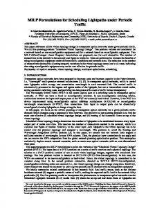
(12) by means of a piecewise-linear one. It is well-known that there are several different ways for doing this; one is represented points in the interval in Fig. 1, where are chosen (such that and ), and a convex, piecewise-linear upper approximation of , which coincides with the latter in the chosen points, is used to replace the original nonlinear objective function. This results in an MILP which differs from UC (for each and ) only in the ). following details (let new variables are introduced together with constraints •

(13) • The cost coefficient of in the objective function is changed to . representing the • Each variable is given a linear cost and value linear function with value 0 when when , i.e.,

Fig. 1. Piecewise-linear approximation of f (p) in the (p; u) space.

and lower approximations constructed in this way only work space, as in in the -space; thus, when represented in the Fig. 1, one notices that the objective function of the new problem is linear along all segments of extremes ( , 0) and ( , 1) for any feasible production level , always with the same slope (in the , , , ). figure, Although the previous linearization is quite natural, it arguably is not the best possible approximation of the objective function of UC; indeed, a different possibility is suggested in in the interval [5]. Arbitrarily choosing points , a different way for producing an MILP which approximates UC is (for each and ) as follows. • Each term of the form (12) is removed from the objective function and replaced with a corresponding new variable ; other terms in the objective function not containing and , e.g., those related to variable startup costs [13], are kept untouched. constraints of the form •

(14)

The MILP approximation of the quadratic function is therefore obtained by replacing (12) with

subject to the original constraints of the problem plus the extra constraints (13). We will refer to this approximated MILP formulation of UC as the standard piece-wise formulation (SPWF). There are different choices for the linearization; for instance, it is easy to construct a lower approximation which is tight to in both function and derivative values in points “in the middle” of the intervals. Most often, the articles where linearization is touted (e.g., [7]–[10]) do not explicitly state how exactly the linearization is constructed, although sometimes this may be deduced; for instance, [7, Fig. 1] most likely indicates the same upper approximation as in SPWF. For the purpose of the present paper, there is no substantial difference between an upper or a lower approximation, as discussed below. Indeed, both upper

, , respectively, are added to the with formulation. We will refer to the above as the perspective-cut (approximate) formulation (PCF) of UC. This choice is justified by a sophisticated theoretical analysis which for the sake of clarity cannot be repeated here; the interested reader is referred to [5] for full details. Here we will just briefly illustrate the basic ideas underlying the construction, in order to clarify in what sense the above choice is, at least in theory, preferable to others, and what are its main differences w.r.t. the previous approach. in (12) is in principle only relevant The function of its (disconnected) domain at points ; however, standard branch-and-bound approaches typically solve the continuous relaxation of the provided formulation, where is allowed to take values in [0, 1] rather than {0, 1}, in order to derive lower bounds on the optimal value of the problem. It thus makes sense to study which formulation provides the best possible (workable) convex relaxation of UC. While such a question does not admit any easy answer for the UC problem in its entirety, it can be answered if one restricts


109

Fig. 3. Piecewise-linear approximation of h(p; u).

Fig. 2. Perspective function of f (p).

himself to the “basic blocks” of the problem; in fact, the convex over , that is, the convex function with the envelope of smallest (in set-inclusion sense) epigraph containing that of , can be shown [5] to be if and if otherwise.

(15)

This function is strongly related with a well-known object in convex analysis, the perspective function of . The epigraph of defines a cone pointed in the , as depicted in origin and having as “lower shape” that of is the section of the cone corresponding to . Fig. 2; Since , it is immediate to verify that for all , that is, is a better objective function, ; indeed, elementary for a continuous relaxation, than over calculus shows that the maximum of is , attained at [ , 1/2]. However, using as the objective function has a serious drawback: it is even a , which we already aim “more nonlinear” function than at making “less nonlinear.” Yet, it is well-known that every convex function is the pointwise supremum of affine functions; for our case these can be easily characterized. Indeed, [5, Theorem 1] shows that the episatisgraph of is composed of all and only triples , and the infinite system fying . We refer of linear inequalities (14), for all to each inequality in (14) as a perspective cut (P/C); as illustrated in Fig. 3, it defines the unique supporting hyperplane to the function passing from (0, 0) and ( , 1). Note that the epigraph of is a cone, i.e., differently from the previous case (cf. Fig. 1) the function is linear along all segments of extremes (0, 0) and ( , 1) for any feasible production level (with varying slope), as it is easy to verify algebraically. Thus, the PCF formulation corresponds to choosing supporting hyperplanes tangent both in (0, 0) and in the points ( , 1), to the graph of and using as objective function the polyhedral function which is the point-wise maximum of the corresponding linear functions; this better describes the true behavior of the actual nonconvex objective function, up to the extent possible to a convex approximation.

Given the standard mixed-integer nonlinear program formulation of UC, PCF is even slightly simpler to implement than SPWF. The differences between SPWF and PCF can be summarized as follows. • Assuming pieces are constructed for each and , SPWF more continuous variables and has more constraints (counting box constraints) than UC, more continuous variables while PCF has only more constraints than UC; thus, PCF has and significantly fewer variables and constraints than SPWF, especially as grows, although the constraints (14) are slightly denser than box constraints. • Since the objective function of PCF underestimates , solving the continuous relaxation of PCF provides a valid lower bound to the optimal value of UC, and therefore the global lower bound provided by a branch-and-bound approach using PCF is valid for UC; this is not true for SPWF if, as in our experiments, its objective function is constructed to be an upper estimate of . This would make a difference, in theory, if the stopping criterion of the branch-and-bound would be computed by evaluating feasible solutions with the value of the “true” objective function (1); in this case, in fact, the solution found would be guaranteed to be optimal to the prescribed accuracy for PCF, but not for SPWF. This could be easily solved by using a lower approximation in SPWF, but anyway it is immaterial for the current approach, that in both cases is a heuristic one, as discussed below. • PCF is well-suited to work with a dynamic , the number of constraints controlling how accurately the objective function is represented. In fact, one can choose a small set of initial constraints, solve the continuous relaxation of PCF , check whether the solution satand, if isfies the P/C (14) for ; if not, the thus obtained cut can be added to the formulation, using the standard mechanisms that MILP solvers make available for implementing the so-called “branch-and-cut” approaches with user-defined cuts. Thus, any required degree of approximation of the original objective function to UC can be obtained without starting with a formulation with a very large . A similar process could in theory be implemented for SPWF; however, while dynamically adding constraints to a formulation during a Branch&Bound is now possible in all current MILP solvers, adding variables is not usually supported. Thus, while a dynamic version of PCF is easily and effectively implemented with current software, imple-

110


menting a dynamic version of SPWF would require a much larger effort. Apart from these differences, the two formulations share the largest part of their variables and constraints, and therefore once one of the two has been programmed, the other can be quite easily obtained with a few modifications, especially if using a high-level algebraic modeling system. Also, because the approach applies to a “very basic” portion of the UC problem, it can be easily applied to the numerous variants of the problem developed in the vast literature on the subject. Finally, the new formulation can be easily applied to the case where the cost function is piecewise-quadratic but non-convex, like for instance the case when valve points need to be taken into account; simply, the approach is applied separately to each segment where the function is convex. IV. COMPUTATIONAL EXPERIENCES In this section we present some numerical results aimed at testing the effectiveness of the P/C-based formulations within heuristic approaches to UC. For this, we implemented three different approaches. equidistant • SPWF: the MILP formulation, with points, is constructed and passed to an MILP solver. • PCF: same as before, but the P/C formulation is used. : initially, the P/C formulation with only two • and , is pieces, the ones corresponding with constructed; additional cuts, up to a maximum of (a user-configurable parameter) per variable are then dynamically generated when needed as described in the previous paragraph. The tests have been performed on an Opteron 246 (2 GHz) computer with 2 GigaBytes of RAM, running Linux Fedora Core 3, and using the highly regarded commercial solver Cplex 9.1. As all current commercial solvers, Cplex offers mechanisms (the cut callback functions) allowing easy implementation of the approach. A crucial parameter to be tuned for this kind of approaches is the prescribed relative accuracy obtained which the solver is allowed to stop: we tested all methods with two settings, a relatively “relaxed” one of 0.5% (the value used in [7], [11]), and the “tighter” 0.01% (the default value for Cplex, considered a very high accuracy). We should mention that for none of the approaches there is an a priori guarantee that the obtained integer solution will in fact be accurate with that precision; this is because the MILP solver stops when its perceived gap is less than the given threshold, but that gap does not accurately measure the true one. In fact, for SPWF the lower bound is not a priori valid, being the objective function of the MILP an upper approximation of (1); by the same token, however, the upper bound is a valid one. The converse obviously happens for PCF, since in that case the objective function of the MILP is a lower approximation of (1). All this is immaterial in practice, since the difference between the actual function value and its (both upper and lower) approximations was always very small, to the tune of 0.01%. However, to make the comparison absolutely fair the gaps reported in the following Tables have been computed by reevaluating the objective function value of the integer solution

provided by the solver using the “true” quadratic objective function (1), and comparing it with the best valid lower bound we know for each instance; since the same lower bound is used for both formulations (note that SPWF does not provide any valid lower bound for (1)), any difference in gaps is only due to the quality of the corresponding feasible solutions. For our tests, we have used two sets of randomly generated realistic pure thermal and hydrothermal instances, with a number of thermal units ranging from 10 to 200 and a number of hydro . units ranging from 10 to 100, on a daily problem These have been generated with a modified version of the procedure described in [16], which produces a generating set with “small,” “medium,” and “large” thermal units in realistic proportions; the characteristics of each unit are then randomly generated within a set of realistic parameters, depending on the type of the unit. The procedure has only been modified to also randomly generate realistic ramping restrictions, resulting in large units to require between two and three hours to ramp from the technical minimum to the technical maximum. For simplicity, all the instances have time-invariant start-up costs; introducing time-dependent startup costs in the MILP formulations is done in the same way for both, and results in the same increase of the number of constraints, thereby it should not materially impact on the comparison between SPWF and PCF. The UC instances are freely available at the OR-Library [17], and have already been used in [6] and [11] for testing Lagrangian relaxation approaches and MIQP- and MILP-based ones. The size of the different MILP formulations tested is reported in Table I; column “ ” reports the total number of thermal generating units, while column “ ” reports the total number of hydro , is therefore comunits. The first half of the table, with posed by “pure thermal” instances; each row reports averaged results of five instances of the same size. Column “bvar” reports the number of binary variables (equal for all formulations), while columns “cvar” report the number of continuous variables for, respectively, SPWF and all the P/C-based formulations. Then, columns “const” report the number of (nonbox) forconstraints for, respectively, SPWF, PCF, and the mulations; for the latter, this is the initial number, i.e., comprising only two P/Cs for each variable. Finally, columns “P/Cs” report the number of P/Cs dynamically generated by and , respectively, when the optimality tolerance is set to the “tight” value of 0.01% (the number is clearly lower with the “relaxed” tolerance of 0.5%). A. Comparing Static Formulations at Lower Accuracy We first analyze the results obtained by comparing SPWF and PCF with stopping criterion at 0.5%. The results are displayed in Table II; columns “SPWF” report results for the SPWF formulation, while columns “PCF” report results for the PCF formulation. In both cases, column “time” reports the required running time (in seconds), column “nd” reports the number of visited nodes in the enumeration tree, and column “LPs” reports the total number of LP solved; this is much larger than the number of nodes because Cplex 9.1 employs a sophisticated “branch-and-cut” approach where valid inequalities are automatically derived and added to the formulation to improve


TABLE I DIMENSIONS OF THE DIFFERENT MILP FORMULATIONS

TABLE II COMPARING SPWF AND PCF FOR LOW ACCURACY

TABLE III COMPARING PCF, PCFD , AND PCFD

111

FOR

LOW ACCURACY

hydrothermal instances typically have smaller gaps than pure thermal ones; this has always been the case in our experience (e.g., [11]). Intuitively, the reason is likely to be that hydro units give the model more flexibility to adapt to the discontinuities caused by the combinatorial nature of thermal units’ operations. B. Static versus Dynamic Formulations at Lower Accuracy

the lower bound. Furthermore, column “gap” reports the obtained gap (in percentage) between the (true) objective function value of the integer feasible solution reported by the formulation and the best valid lower bound we know for each instance. Finally, column “rgap” reports the obtained gap (in percentage) between the lower bound obtained at the root node of the enumeration tree (solving the continuous relaxation of the MIP formulation), compared to the best valid upper bound we know for each instance; since the same upper bound is used for both formulations, the gaps can be compared. The table shows that both SPWF and PCF obtain good quality solutions; most often, PCF attains solution of slightly better quality than SPWF. Furthermore, PCF most often terminates significantly faster. This is partly due to the fact that solving the continuous relaxation of PCF is slightly but noticeably faster than solving that of SPWF (this fact is not reported in the table due to space reasons), and to a larger extent due to the better root node gap (cf. column “rgap”). Although the difference may look minor, the reduction in root node gap is significant enough to diminish the total number of LPs solved, and often the number of branch-and-bound nodes, too, finally yielding a consistently reduced running time. This confirms the better quality of the lower bound produced by the PCF formulation w.r.t. that produced by the SPWF formulation, despite the fact that the latter is not even a guaranteed lower bound since the original objective function is upper approximated. The table also shows that

Having proven that PCF is a worthy competitor for SPWF, we now proceed at testing the impact of dynamic versus static generation of the P/C. For this, we compare PCF with two variants of , for and , respectively. has the same maximum size as PCF, but cuts are generated only when needed, and therefore can “concentrate” on some “critical” variables, while leaving others (e.g., those that always attain zero value in the continuous relaxation) with a less accurate, but still sufficient, approximation of the objective function; furthermore, the points where the cuts are evaluated are chosen dynamically allows for arbiby the approach instead of a priori. trarily accurate approximations of the objective function, possibly paying a high price in terms of the size of the linear programs that need be solved at each node of the enumeration tree. The results are displayed in Table III, where the meaning of the columns is the same as in the previous one. The table shows interesting results. Both dynamic approaches are competitive with the static one. In particular, it appears that is remarkably effective for small- to mid-scale inis more effective on the large-scale ones; stances, while for the largest hydrothermal instances it provides slightly better solutions in half of the time required by PCF. This is probably due to the fact that for moderate size instances the more accurate approximation leads to finding a better solution quicker, but as the size of the instances grows large the increase in the computational cost of the solution of the linear programs corresponding to the many more P/C added overbalances the improvements in accuracy of the objective function. All in all, however, the results clearly show that an appropriate choice of the parameter leads to substantially better results w.r.t. the static formulation. C. Results With Higher Accuracy Finally, we analyze the impact of the optimality threshold by presenting the results for all four approaches (SPWF and the three P/C-based ones) with the “tighter” stopping tolerance of 0.01%. Since attaining such a high accuracy may require a

112


TABLE IV COMPARING SPWF AND PCF FOR HIGH ACCURACY

V. CONCLUSIONS AND DIRECTIONS FOR FUTURE WORK In this paper, we have proposed a new way for constructing MILP approximated formulations for hydrothermal unit commitment problems. While being not more difficult to implement than previously proposed formulations, the new approach significantly improves the performances of MILP-based heuristics to the problem, either in terms of required running time, or in terms of quality of the obtained solutions. With a limited additional implementation effort dynamic versions of the approach can be implemented which may lead to further significant improvements of the results. While the formulation is tested only on a “standard” form of the UC problem, the underlying concept can be applied to many other variants of the problem, where analogous results should be expected. All in all, these results show that appropriate formulations of UC problems can be used to find good-quality solutions in relatively short time by using off-the-shelf, general-purpose optimization software.

very long time, the search is stopped after 10 000 s and the best solution obtained so far is returned. The results are displayed in Table IV; the meaning of the columns in this table is the same as in the previous ones. As the table shows, allowing the search to continue decreases the final gap by a significant factor; it does not necessarily bring it down to 0.01%, even in the (few) instances that are solved up to the prescribed accuracy, due to the fact that the MILP formulations are only approximations of the “true” MIQP one. However, the improvement in accuracy comes at the expense of a dramatic increase of running times; all but the smallest instances are stopped by the time limit, not a surprising result in view of the experiments reported in [5]. All the formulations attain similar results; however, for the small-scale instances that are solved up to the prescribed accuracy within the allotted time limit the P/C-based formulations are most often (slightly but noticeably) faster, while providing comparable or better solutions. For the other instances, within the same total running time the P/C-based formulations are able to attain slightly better final solutions on large-scale pure thermal instances, and are competitive on all other cases. The P/C-based formulations are also competitive for hydro-thermal instances, which however are solved with a very high degree of accuracy by both methods; the final gaps are only fractionally larger than 0.01%, and the algorithms cannot stop only because the lower bound computed by the MILP formulations is not as accurate as the one used for computing the table, which is based on sophisticated Lagrangian techniques [11]. Among the P/C-based formulations, appears to be the more “robust,” as it almost always reports—for a given running time—solutions of equivalent or (slightly) better quality than all the others. In general, the results show that the PCF formulation provides, with the same effort, a better description of the feasible region (objective function) of the “true” MIQP problem, which finally leads, ceteris paribus, to shorter running times and/or better feasible solutions. Allowing the number of P/Cs used, and the points where they are generated, to be dynamic further significantly improves the efficiency of the approach, especially if the allowed maximum number of cuts is properly managed.

REFERENCES [1] A. J. Wood and B. F. Wollemberg, Power Generation Operation and Control. New York: Wiley, 1996. [2] B. F. Hobbs, M. Rothkopf, R. P. O’Neill, and H. P. Chao, The Next Generation of Unit Commitment Models. Boston, MA: Kluwer, 2001. [3] J. M. Arroyo and A. J. Conejo, “Optimal response of a thermal unit to an electricity spot market,” IEEE Trans. Power Syst., vol. 15, no. 3, pp. 1098–1104, Aug. 2000. [4] A. Borghetti, A. Frangioni, F. Lacalandra, C. Nucci, and P. Pelacchi, “Using of a cost-based unit commitment algorithm to assist bidding strategy decisions,” presented at the Proc. IEEE 2003 Powertech Bologna Conf., 2003, Paper no. 547, Borghetti, A., Nucci, C.A., and Paolone, M., Eds., unpublished. [5] A. Frangioni and C. Gentile, “Perspective cuts for a class of convex 0–1 mixed integer programs,” Math. Program., vol. 106, no. 2, pp. 225–236, Apr. 2006. [6] A. Frangioni and C. Gentile, “Solving nonlinear single-unit commitment problems with ramping constraints,” Oper. Res., vol. 54, no. 4, pp. 767–775, Jul.–Aug. 2006. [7] M. Carrión and J. M. Arroyo, “A computationally efficient mixed-integer linear formulation for the thermal unit commitment problem,” IEEE Trans. Power Syst., vol. 21, no. 3, pp. 1371–1378, Aug. 2006. [8] G. W. Chang, M. Aganagic, J. G. Waight, J. Medina, T. Burton, S. Reeves, and M. Christoforidis, “Experiences with mixed integer linear programming based approaches on short-term hydro scheduling,” IEEE Trans. Power Syst., vol. 16, no. 4, pp. 743–749, Nov. 2001. [9] O. Nilsson and D. Sjelvgren, “Mixed-integer programming applied to short-term planning of a hydro-thermal system,” IEEE Trans. Power Syst., vol. 11, no. 1, pp. 281–286, Feb. 1996. [10] Z. Yu, F. T. Sparrow, B. Bowen, and F. J. Smardo, “On convexity issues of short-term hydrothermal scheduling,” Elect. Power Energy Syst., vol. 22, no. 6, pp. 451–457, Aug. 2000. [11] A. Frangioni, C. Gentile, and F. Lacalandra, “Solving unit commitment problems with general ramp constraints,” Int. J. Elect. Power Energy Syst., vol. 30, no. 5, pp. 316–326, Jun. 2008. [12] S. de la Torre, J. M. Arroyo, A. J. Conejo, and J. Contreras, “Price maker self-scheduling in a pool-based electricity market: A mixedinteger LP approach,” IEEE Trans. Power Syst., vol. 17, no. 4, pp. 1037–1042, Nov. 2002. [13] M. P. Nowak and W. Römisch, “Stochastic Lagrangian relaxation applied to power scheduling in a hydro-thermal system under uncertainty,” Ann. Oper. Res., vol. 100, no. 1–4, pp. 251–272, Dec. 2000. [14] J. M. Arroyo and A. J. Conejo, “Modeling of start-up and shut-down power trajectories of thermal units,” IEEE Trans. Power Syst., vol. 19, no. 3, pp. 1562–1568, Aug. 2004. [15] A. Borghetti, A. Frangioni, F. Lacalandra, and C. Nucci, “Lagrangian heuristics based on disaggregated bundle methods for hydrothermal unit commitment,” IEEE Trans. Power Syst., vol. 18, no. 1, pp. 313–323, Feb. 2003.


[16] A. Borghetti, A. Frangioni, F. Lacalandra, A. Lodi, S. Martello, C. Nucci, and A. Trebbi, “Lagrangian relaxation and tabu search approaches for the unit commitment problem,” presented at the Proc. IEEE 2001 Powertech Porto Conf., 2001, Paper no. PSO5-397, Saraiva, J. T. and Matos, M. A., Eds., unpublished. [17] J. Beasley, [Online]. Available: http://www.people.brunel.ac.uk/~mastjjb/jeb/orlib/info.html, 1990

Antonio Frangioni received the Computer Science degree with honors and the Ph.D. degree in computer science from the University of Pisa, Pisa, Italy, in 1992 and 1996, respectively. He was a Research Associate at the Computer Science Department of the University of Pisa from 1996 to 2004, where he is now an Associate Professor. His main research interests are in models and algorithms for large-scale continuous and combinatorial optimization problems, using such techniques as decomposition algorithms, interior-point methods, reformulation techniques, and network flow approaches. He is author and coauthor of more than 25 publications among journal papers and book articles, plus several conference presentations.

113

Claudio Gentile received the Computer Science degree with honors from the University of Pisa, Pisa, Italy, in 1995 and the Diploma from the Scuola Normale Superiore of Pisa. In 2000, he received the Ph.D. degree in operations research from the University “La Sapienza” of Rome, Rome, Italy. Since 1999, he has been a Researcher at the Institute of System Analysis and Computer Science “Antonio Ruberti” of the Italian National Research Council (IASI-CNR), Rome. His main research interests are in combinatorial optimization, polyhedral theory for linear and nonlinear integer programming problems, interior point methods, and network flow problems. He is coauthor of more than ten publications among journal papers and book articles, plus some in conference proceedings.

Fabrizio Lacalandra received the Electrical Engineering degree from the Polytechnic of Bari, Bari, Italy. He also studied at the Tampere University of Technology (SF), Tampere, Finland. Since 2000, he has worked as a Quantitative Analyst with different companies in various fields. At the present time, he is Head of the Quantitative Unit of Titian Global Investments LLP, London, U.K.. Prior to joining Titian, he , Pisa, has been a Technical Director with pti Italy, in charge of the ower ched suite, and he has also been an External Consultant for RIE-srl (Bologna) as a “Matter Expert.” His primary research interests are in continuous and combinatorial optimization, mainly applied to electricity operation problems, the broader electricity market, and advanced finance portfolio models. He is coauthor of some publications published on reviewed journals, plus some publications in conference proceedings.