Time Algorithm for the Restricted Scaffold Assignment Problem

An O(n log n)-Time Algorithm for the Restricted Scaffold Assignment Problem Justin Colannino Mirela Damian Ferran Hurtado John Iacono Henk Meijer Suneeta Ramaswami Godfried Toussaint

Abstract The restriction scaffold assignment problem takes as input two finite point sets S and T (with S containing more points than T ) and establishes a correspondence between points in S and points in T , such that each point in S maps to exactly one point in T , and each point in T maps to at least one point in S. In this paper we show that this problem has an O(n log n)time solution, provided that the points in S and T are restricted to lie on a line (linear time, if S and T are presorted).

1

Introduction

Consider two finite sets of points S and T with the cardinality of S greater than the cardinality of T , and total cardinality n. The objective of the restriction scaffold assignment problem is to establish a correspondence between the points in S and the points in T , such that each point in S corresponds to exactly one point in T , and each point in T corresponds to at least one point in S. This correspondence is measured by a cost function δ that assigns a cost δ(s, t) to each assigned pair (s, t). The cost of an assignment is the sum of the costs of all assigned pairs. The goal of this assignment problem is to find an assignment of minimum cost. This assignment problem is also known as the many-to-one assignment problem. The one-to-one version of the assignment problem requires that each point in S be assigned to exactly one point in T and each point in T be assigned exactly one point from S. Throughout the paper, whenever we write about the assignment problem, we refer to the many-to-one version of the problem. The simplest version of the assignment problem assumes that the points in S and T lie on a line and the cost function is the distance betwen pairs of points in the L1 metric. In this setting, the one-to-one assignment problem has a simple 1

O(n log n) time solution when |S| = |T |: first sort the points in O(n log n) time, then assign the k th point in S to the k th point in T in O(n) time [5], [14]. However, the situation |S| < |T | arises in many practical applications. This situation was first addressed by Karp and Li [9], who provided an O(n log n) time algorithm for the one-to-one assignment problem (O(n) time, if S and T are given in sorted order). Simpler and equally efficient solutions have later been provided in [1, 3, 16]. Eiter and Mannila [7] studied the assignment problem in the context of measuring the distance between two theories expressed in a logical language. They showed that for points in arbitrary dimensions, this problem has an O(n 3 ) time solution that uses the Hungarian method [11]. When the points are restricted to a line, a minimum cost assignment can be used in measuring the similarity between musical rhythms. In this context, Toussaint [15] proposed the use of the swap distance as a similarity measure when S and T have equal cardinalities. For the case of unequal cardinalities he generalized the swap distance to the directed swap distance, where the “direction” of the assignment (surjection) is from the larger set to the smaller set. This similarity measure has since been successfully applied to a phylogenetic analysis of Flamenco metric patterns [5]. If the onsets of a rhythm are represented as points on a line separated by “silence” intervals, the directed swap distance between two rhythms represented by the sets S and T is precisely the cost of an optimal assignment between S and T , with underlying cost function L 1 . The preceeding assignment problem has also been solved as a more general instance of bibranchings first instroduced by Schrijver [12]. Let D = (V, E) be a directed graph, and let V be partitioned into two disjoint sets, the source vertices S and the target vertices T . A bibranching in D with respect to S is a set of edges B in E such that: for each v in S, B contains a directed path from v to a vertex in T , and for each v in T , B contains a directed path from a vertex in S to v. For the special case when D is a bipartite graph with color classes S and T , and all the edges in D are directed from S to T , the bibranching is a bipartite edge cover. Furthermore, the minimum weight bipartite edge cover in this setting corresponds to our assignment problem. Keijsper and Pendavingh [10] describe an O(|E|) time algorithm attributed to J. F. Geelen for reducing the minimum weight bipartite edge cover problem to the maximum weight matching problem. They also describe a solution for the latter problem that uses shortest path algorithms from [6] and [13] sped up with Fibonacci heaps [8]. Their algorithm runs in time O(n0 (|E| + n log n)), where n0 = min{|S|, |T |}. In our problem this complexity is O(n3 ) in the worst case, matching the complexity of the approach of Eiter and Mannila. However, the algorithm of Eiter and 2

Mannila is simpler. The preceeding assignment problem also appears as the restriction scaffold assignment problem in computational biology [2]. The goal here is to establish a correspondence between sparse experimental data and a restricted set of known structural building blocks. Ben-Dor et. al. [2] model the restriction scaffold assignment as an assignment problem for points on a line, and suggested an O(n log n) time algorithm to solve this problem. However, Colannino and Toussaint [4] showed that this algorithm sometimes fails to yield a minimum cost assignment. Thus, the best existing solution to the assignment problem in one dimension is the O(n2 ) algorithm given in [4]. In this paper, we show that the many-to-one assignment problem with underlying cost function L1 in one dimension can be solved in O(n log n) time (O(n) if the points in S and T are given in sorted order). Our algorithm is a simple extension of the O(n log n) time algorithm of Karp and Li [9] for finding the minimum cost one-to-one assignment.

2

Background

Let S = {s0 , s1 , s2 , . . .} and T = {t0 , t1 , t2 , . . .} be two finite sets of points that lie on a horizontal line, with |S| + |T | = n and |S| > |T |. For any s ∈ S and t ∈ T , the cost δ(s, t) of an assigned pair (s, t) is the absolute value of the difference between the x-coordinates of s and t. To avoid overloading the notation, we use the same symbol for a point and its x-coordinate. Thus, δ(s, t) = |s − t|. We assume that si < si+1 , 0 ≤ i < |S| − 1 and tj < tj+1 , 0 ≤ j < |T | − 1. An assignment A between S and T consists of pairs of points (s, t) (henceforth edges), with s ∈ S and t ∈ T , such that each point in S belongs to exactly one edge in A, and each point in T belongs to at least one edge in A. The cost of A is X cost(A) = δ(s, t) (s,t)∈A

Our goal is to find an assignment A of minimum cost. If two points in S ∪ T have the same x-coordinate, we can slightly shift one of them to the left or right. If the minimum cost assignment is unique and the change is sufficiently small, this change will not affect the optimal assignment. If there are several assignments with the same optimal cost, at least one of them will be the optimal solution of the new point set. So we may assume without loss of generality that all points in S ∪ T are distinct.

3

2.1

Preliminaries

For any s ∈ S and t ∈ T , the value |s − t| can be expressed in a different way as follows. Define a function fs,t to be 1 in the interval between s and t and 0 R +∞ at any other point (see Figure 1). Then |s − t| = −∞ fs,t (x)dx. y=1

y=0

s

t

Figure 1: Function fs,t . Shaded area represents the cost |s − t|. The cost of an assignment A is therefore Z X Z +∞ fs,t (x)dx = cost(A) = fA (x) =

X

fs,t (x)dx

−∞ (s,t)∈A

(s,t)∈A −∞

If we define

+∞

X

fs,t (x)

(s,t)∈A

then the value fA (a) is simply the number of edges in A pierced by the vertical line x = a, and the cost of A is Z +∞ fA (x)dx (1) cost(A) = −∞

Our definition of fA is similar in nature to the height function H : R → Z introduced by Karp and Li [9]. Informally, they define H(a) at each point a as the difference between the number of points in S and the number of points in T restricted to the interval (−∞, a] (or equivalently, to the left of the vertical line x = a). Thus H remains constant throughout each interval that does not contain a point in S ∪ T . Figure 2 shows the stair-shaped curve of H for a small example. Note that up transitions in the curve correspond to points in S and down transitions correspond to points in T . We refer to the value H(x) as the height of x. Note that H(∞) = |S| − |T |. R +∞ Lemma 1 If |S| = |T |, then −∞ |H(x)| dx is the cost of the assignment that assigns the k th largest element of S to the k th largest element of T . Proof: Follows immediately from (1) and the fact that, for this particular assignment, fA (x) = |H(x)| at each point x. Figure 3a shows an assignment for two sets S and T , with |S| = |T |. The cost of this assignment is equal to the area shaded in Figure 3b, which is precisely R +∞ the value of the integral −∞ |H(x)| dx. 4

2 0

3

1

11 4

6

12

13

14

10

8

15

16 17

Figure 2: Height function for sets S = {0, 3, 4, 6, 13, 14, 15, 16} and T = {1, 2, 8, 10, 11, 12}. 4

0

6

13

14

16

(a) 1

2

2 0

1

8

4 6

10

11

12

10

11

12

13

14

16

(b)

8

Figure 3: (a) One-to-one assignment for sets S = {0, 4, 6, 13, 14, 16} and T = {1, 2, 8, 10, 11, 12} (b) Shaded area represents the cost of the assignment.

3

Properties of a Minimum Cost Assignment

Our algorithm for computing a minimum cost assignment A exploits several important properties of A, which we discuss next. A crossing is defined by a pair of edges (a, d) and (b, c) such that a < b in S and c < d in T . Lemma 2 There exists a minimum cost assignment with no crossings. Proof: Let A be a minimum cost assignment between S and T with a minimum number of crossings. If A has zero crossings, the proof is finished. Otherwise, pick two crossing edges (a, d) and (b, c) in A, with a < b in S and c < d in T . We show that A0 = A \ {(a, d), (b, c)} ∪ {(a, c), (b, d)} is an assignment with cost(A0 ) ≤ cost(A), a contradiction. In particular, we show that f A0 (x) ≤ fA (x) at each point x; then cost(A0 ) ≤ cost(A) follows immediately from (1). First note that fA0 (x) ≤ fA (x) is true for any x such that the vertical line L at x intersects neither of (a, d) and (b, c). Suppose now that L intersects (a, c). Then L must also intersect either (a, d) (see Figure 4a) or (b, c) (see Figure 4b) or both (see Figure 4c). Similarly, if L intersects (b, d), then L also intersects at least one of (a, d) and (b, c). Furthermore, if L intersects both (a, c) and 5

(b, d), then L also intersects both (a, d) and (b, c) (see Figure 4c). It follows that fA0 (x) ≤ fA (x). a

a

b

L

c

c

d

(a)

b

a

d

L

c

d

(b)

b

L

(c)

Figure 4: (a) Vertical line L intersects (a, c) and (a, d) (b) L intersects (a, c) and (b, c) (c) L intersects (a, c), (b, d), (a, d) and (b, c). An assignment A can also be regarded as a function A : S → T such that A(s) = t for each (s, t) ∈ A. For any t ∈ T , let A −1 (t) denote the set of elements s ∈ S such that A(s) = t. For each point s ∈ S, define the nearest neighbor N (s) to be point in T closest to s, i.e, |N (s)−s| ≤ |t−s| for any t ∈ T . In the case of a tie, N (s) is arbitrarily picked from among the two candidate neighbors. Lemma 3 Let A be optimal and let t ∈ T be such that A −1 (t) contains two or more elements. Then for each s ∈ A−1 (t), t is a nearest neighbor of s. Furthermore, T contains no points in between s and t. Proof: Assume to the contrary that there is s ∈ S with A(s) = t, |A −1 (t)| > 1, and N (s) 6= t. Refer to Figure 5. Define a new assignment A 0 with A0 (s) = N (s) and A0 (x) = A(x) for x 6= s. Note that A0 is also an assignment: A−1 (t) contains at least one point. Also cost(A 0 ) = cost(A) − |s − t| + |s − N (s)| (see Figures 5a and 5b). Since |s−N (s)| < |s−t|, it follows that cost(A 0 ) < cost(A), s

s

S

S

T

T N(s)

t

N(s)

(a)

t

(b)

Figure 5: (a) Assignment A with A(s) 6= N (s) (b) Assignment A 0 with A0 (s) = N (s) contradicting the fact that A is of minimum cost. Thus, t is a nearest neighbor of s. 6

The claim that T contains no points in between s and t is immediate: if such a point t1 ∈ T existed, then |s − t1 | < |s − t|, contradicting the fact that N (s) = t. Observe that for any subset R ⊂ S of size |R| = |S| − |T |, there is a unique minimum cost assignment (with no crossings) from S \R to T . Let A S\R denote the edges of such an assignment, and define a new assignment A R : S → T as follows: ( N (x) if x ∈ R, (2) AR (x) = y if x ∈ S \ R and (x, y) ∈ AS\R Lemma 3 implies that there always exists a subset R such that A R defines a minimum cost assignment from S to T . Furthermore, R satisfy a special height condition, stated in the lemma below. Lemma 4 There exists a subset R ⊂ S with |R| = |S| − |T | such that A R defines a minimum cost assignment from S to T , and the k th smallest element of R has height k. Proof: Let A : S → T define a minimum cost assignment. We prove the existence of AR by constructing a set R ⊂ S with the properties stated in this lemma. Initially R is empty. If |A−1 (t)| = 1 for all t ∈ T , then R is empty and the proof is finished. Otherwise, we process points t ∈ T for which A −1 (t) has two or more elements. For each such point we consider two cases, as depicted in Figure 6. If all points in A−1 (t) are less than t, then we add to R all but the largest (rightmost) point in A−1 (t) (see Figure 6a). Otherwise, we add to R all points in A−1 (t) except for the smallest (leftmost) point greater than t (see Figure 6b). Insert in R

Insert in R

S

S

T (a)

T

t

t

(b)

Figure 6: (a) All points in A−1 (t) are less than t. (b) Some points in A −1 (t) are greater than t. We now define AR as in (2). Since AR is identical to A, AR is a minimum cost many-to-one assignment from S to T . 7

It remains to show that the k th smallest element of R has height k. To see this, first consider the smallest element of a nonempty set A −1 (t) ∩ R. Call this element r and suppose it is the k th smallest element of R. It follows then that (i) R contains k − 1 points less than r, and (ii) T and S \ R contain an equal number of elements less than r. This latter claim follows from Lemma 3, which tells us that T contains no elements in between r and t, and the following observation: the way in which we have selected R ensures that if t lies to the left of r (i.e., t < r), the assigned item for t in S/R lies to the left of r, and if t lies to the right of r (t > r), the assigned item for t in S/R lies to the right of r. These together imply that H(r) = k. We now show that the points in A−1 (t) \ {r} have height values k + 1, k + 2, . . ., in order from smallest to largest. By Lemma 3, T contains no points in between s and t, for each s ∈ A−1 (t). Then the points in R ∩ A−1 (t) have incrementally increasing height values. It follows that the height of the k th smallest element of R is k. Let HR represent the height function restricted to sets S \R and T . This means that for each x, HR (x) is the difference between the number of points in S \ R and the number of points in T restricted to the interval (−∞, x]. Lemma 5 The cost of assignment AR is Z +∞ X |HR (x)|dx |r − N (r)| +

(3)

−∞

r∈R

Proof:R By Lemma 1 we have that the contribution of S \ R to the cost of +∞ AR is −∞ |HR (x)|dx. Since each point inP R maps to its nearest neighbor, the contribution of R to the cost of A R is r∈R |r − N (r)|. These together conclude the lemma. Theorem 6 Let R ⊂ S be a subset of size |R| = |S| − |T | with two properties: i. The k th smallest element of R has height k. ii. R minimizes the quantity from (3). Then AR defines a minimum cost assignment from S to T . Proof: By Lemma 4, we know that there exists a set R that satisfies (i). By Lemma 5, R satisfies (ii). It follows that A R is a minimum cost assignment from S to T . 8

4

Computing a Minimum Cost Assignment

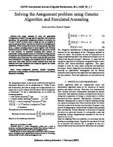
Theorem 6 gives an exact description of the set R that yields a minimum cost assignment AR . We now turn to the problem of efficiently determining this set. With this goal in mind, we introduce the following notation. For any point x and any integer k, define the relative height of x with respect to k as  1, if H(x) ≥ k hk (x) = −1, if H(x) < k Observe that when a point s is removed from S, H(x) decreases by 1 for all x > s. Suppose that H(s) = k, and let m be the largest point in S ∪ T . The removal of s causes the area R m under the height function between s and m to decrease by the quantity s hk (x)dx. We use this observation to define the profit of removing s from S and placing it in R (recall that A R assigns each item in R to its nearest neighbor), as follows: Z m P (s) = hk (x)dx − |s − N (s)| (4) s

2 0

_ _ _ _ _ _ _ _ _ _ _ _

3

1

4

6

+ + + + + + + + + + 10

8

12

13

_ _ _ _ 15

16 17

Rm Figure 7: A depiction of the integral s hk (x)dx for s = 4. The integral represents the effect of excluding 4 from the one-to-one assignment from S to T. The profit function quantifies the benefit of placing s in R, the goal being to minimize the cost of the assignment defined by A R . The integral term in (4) represents the effect of excluding s from the one-to-one assignment from S \ R to T , as depicted in Figure 7. The term |s − N (s)| in (4) represents the cost of assigning s to its nearest neighbor. We minimize the cost of the assignment defined by AR by choosing items s that maximize P (s). This is formalized in the following lemma. Lemma 7 Let R ⊂ S be a set with elements r 1 < r2 . . . < r|S|−|T | such that H(rk ) = k and rk maximizes P (s) among all points s ∈ S of height k. Then R minimizes Z +∞ X |HR (x)|dx |r − N (r)| + −∞

r∈R

9

Proof: Karp and Li [9] proved that any set R of size |S| − |T | whose k th smallest element has height k satisfies the equality Z +∞ Z m XZ m |HR (x)|dx = |H(x)|dx − hk (x)dx −∞

0

r∈R r

Summing up the cost contribution of R to both sides of the equality yields Z m Z +∞ XZ m X X hk (x)dx |H(x)|dx− |HR (x)|dx = |r−N (r)|+ |r−N (r)|+ −∞

r∈R

0

r∈R

r∈R

r

This is equivalent to X

|r − N (r)| +

Z

+∞

|HR (x)|dx =

−∞

r∈R

Z

m

|H(x)|dx −

0

X

P (r)

r∈R

Since P (rk ) is maximized at each height kP and there is only one element in R at each height, we have that R maximizes r∈R P (r), which in turn minimizes X

|r − N (r)| +

r∈R

Z

+∞

|HR (x)|dx

−∞

as required (refer to Lemma 5). The following algorithm uses the preceding lemma to determine the optimal set R, and then compute the minimum cost assignment.

4.1

The Assignment Algorithm

Initially R is the empty set. 1. Sort S and T . 2. Calculate H(x) for each x ∈ S ∪ T . In between consecutive points, H is constant. 3. Calculate P (s) for each s ∈ S. 4. For k = 1, 2, . . . |S| − |T | 4.1 Find the leftmost point rk of height k that maximizes P (rk ). 4.2 Add rk to R. 5. Return AR . 10

Lemma 8 The assignment algorithm computes a minimum cost assignment from S to T . Proof: Let rk be the element of R of height k returned by the algorithm. If we show that r1 < r2 < . . . < r|S|−|T |, then it follows by Lemma 7 that AR is a minimum cost assignment. We prove below, by contradiction, that indeed r1 < r2 < . . . < r|S|−|T |. Let m be the largest point in S. Assume that there exists some k(1 ≤ k ≤ |S| − |T | − 1) for which the algorithm returns r k and rk+1 , with rk > rk+1 . Let sk be the maximal element at height k in S \ R which is less than r k+1 . By continuity, such an sk must exist. Similarly, let sk+1 be the minimal element at height k + 1 in S \ R which is greater than r k . Such an sk+1 must exist since the height at ∞ is H(∞) = |S| − |T |. Refer to Figure 8. rk+1 sk

sk+1 rk

hk (x) > 0

hk+1(x) < 0

Figure 8: sk (sk+1 ) is the closest point at height k(k + 1) to the left (right) of rk+1 (rk ). Since H(rk+1 ) = H(sk+1 ) and rk+1 < sk+1 , we have that Z m Z sk+1 Z m k+1 k+1 hk+1 (x)dx h (x)dx + h (x)dx = sk+1

rk+1

rk+1

From this and equation (4), we can derive the following relation between the profit functions of rk+1 and sk+1 : Z sk+1 P (rk+1 ) = P (sk+1 )+ hk+1 (x)dx−|rk+1 −N (rk+1 )|+|sk+1 −N (sk+1 )| (5) rk+1

Note that equality (5) is the result of breaking up the integral corresponding to P (rk+1 ) into two parts, and taking into account the distance from each element to its nearest neighbor. Similarly, we can derive the following relation between P (rk ) and P (sk ): Z rk hk (x)dx − |sk − N (sk )| + |rk − N (rk )| (6) P (sk ) = P (rk ) + sk

The nearest neighbor of sk cannot be farther than N (rk+1 ). This translates into: |sk − N (sk )| ≤ |rk+1 − N (rk+1 )| + |sk − rk+1 | 11

Also note that hk (x) is positive on the interval (sk , rk+1 ), which allows us to rewrite the previous equation as: Z rk+1 |sk − N (sk )| ≤ |rk+1 − N (rk+1 )| + hk (x)dx (7) sk

Similar arguments lead to the following relationship between nearest neighbors of rk and sk+1 : Z sk+1 hk+1 (x)dx (8) |rk − N (rk )| ≥ |sk+1 − N (sk+1 )| + rk

Finally, on the interval (rk+1 , rk ) note that Z rk Z k+1 h (x)dx ≤ rk+1

rk

hk (x)dx

(9)

rk+1

Let Mk = |sk −N (sk )|−|rk −N (rk )|. Simple arithmetic that involves inequalities (7), (8) and (9) yields Z rk Z sk+1 k h (x)dx − Mk ≥ hk+1 (x)dx + Mk+1 sk

rk+1

This along with (5) and (6) implies that P (sk ) − P (rk ) ≥ P (rk+1 ) − P (sk+1 ) Since rk+1 was picked by the assignment algorithm, we have that P (r k+1 ) ≥ P (sk+1 ). This implies that P (sk ) ≥ P (rk ), but since sk lies to the left of rk , the assignment algorithm would have picked s k instead of rk , a contradiction.

4.2

Complexity Analysis

Sorting in step 1 takes O(n log n) time. All other steps run in O(n) time. The only steps where this is not obvious are steps 2 and 3 that involve computing H(x) and P (x) respectively. H(x) can be computed for all s ∈ S by conducting a sweep of the sorted points in S ∪T , adding one when we encounter an element of S and subtracting one when we encounter an element of T . Since all nearest neighbors of the elements of S can easily be computed in linear time, to show that we can compute the profit function for all elements of S in linear time we concern ourselves only with computing the integral of relative height function hk . This integral can be computed in linear time for all 12

points in S at heightR k in a sweep from right to left. For the rightmost element m sr of S at height k sr hk (x)dx = |sr − m|, where m is the largest point in S. Rm Suppose that we know s hk (x)dx for some item s at height k. Let s 0 < s be the largest element in S also at height k, and let t < s be the largest element in T at height k. Note that by continuity, t exists and must be greater than s 0 . Also note that hk (x) is positive for all s0 ≤ x ≤ t, and hk (x) is negative for all t < x < s. Thus we can derive the following equation: Z m Z m k hk (x)dx + |s0 − t| − |t − s| (10) h (x)dx = s0

s

This value can be computed in constant time for each s 0 ∈ S. Thus we can compute P (s) for all s ∈ S in linear time. It follows that the assignment algorithm runs in O(n log n) time. Furthermore, if S and T are given in sorted order, the assignment algorithm runs in O(n) time.

5

Conclusion

We have shown that the one-to-one assignment algorithm in [9] can be extended to produce a minimum cost many-to-one assignment. The algorithm runs in O(n log n) time, if the input points are given in arbitrary order, and in O(n) time, if the input points are presorted. To our knowledge, this is the first solution to the assignment problem that achieves this time complexity.

References [1] A. Aggarwal, A. Bar-Noy, S. Khuller, D. Kravets, and B. Schieber. Efficient minimum cost matching and transportation using the quadrangle inequality. J. Algorithms, 19(1):116–143, 1995. [2] A. Ben-Dor, R.M. Karp, B. Schwikowski, and R. Shamir. The restriction scaffold problem. Journal of Computational Biology, 10(2):385–398, 2003. [3] S. R. Buss and P. N. Yianilos. Linear and o(n log n) time minimumcost matching algorithms for quasi-convex tours. SIAM J. of Computing, 27(1):170–201, 1998. [4] J. Colannino and G. Toussaint. An algorithm for computing the restriction scaffold assignment problem in computational biology. Information Processing Letters, 95(Issue 4):466–471, 2005. 13

[5] Miguel D´ıaz-Ba˜ nez, Giovanna Farigu, Francisco G´omez, David Rappaport, and Godfried T. Toussaint. El comp´as flamenco: a phylogenetic analysis. In Proceedings of BRIDGES: Mathematical Connections in Art, Music and Science, Southwestern College, Winfield, Kansas, July 30 - August 1 2004. [6] J. Edmonds and R. M. Karp. Theoretical improvements in algorithmic efficiency for network flow problems. Journal of the Association for Computing Machinery, 19:248–264, 1972. [7] Thomas Eiter and Heikki Mannila. Distance measures for point sets and their computation. Acta Informatica, 34(2):109–133, 1997. [8] M. L. Fredman and R. E. Tarjan. Fibonacci heaps and their uses in improved network optimization algorithms. Journal of the Association for Computing Machinery, 34:596–615, 1987. [9] R.M. Karp and S.-Y.R. Li. Two special cases of the assignment problem. Discrete Mathematics, 13(46):129–142, 1975. [10] J. Keijsper and R. Pendavingh. An efficient algorithm for minimumweight bibranching. Journal of Combinatorial Theory, 73(Series B):130– 145, 1998. [11] H. W. Kuhn. The Hungarian method for the assignment problem. Naval Research Logistics, 2:83–97, 1955. [12] A. Schrijver. Min-max relations for directed graphs. Annals of Discrete Mathematics, 16:261–280, 1982. [13] N. Tomizawa. On some techniques useful for the solution of transportation network problems. Networks, 1:173–194, 1972. [14] Godfried Toussaint. A comparison of rhythmic similarity measures. In Proc. 5th International Conference on Music Information Retrieval, pages 242–245, 2004. [15] G.T. Toussaint. Classification and phylogenetic analysis of african ternary rhythm timelines. In Proceedings of BRIDGES: Mathematical Connections in Art, Music and Science, pages 25–36, 2003. [16] M. Werman, S. Peleg, R. Melter, and T. Kong. Bipartite graph matching for points on a line or a circle. J. Algorithms, 7:277–284, 1986.

14