Time-Aware VM-Placement and Routing with. Bandwidth Guarantees in Green Cloud Data Centers. Aissan Dalvandi, Mohan Gurusamy, and Kee Chaing Chua.
2013 IEEE International Conference on Cloud Computing Technology and Science
Time-Aware VM-Placement and Routing with Bandwidth Guarantees in Green Cloud Data Centers Aissan Dalvandi, Mohan Gurusamy, and Kee Chaing Chua Department of Electrical and Computer Engineering, National University of Singapore, Singapore 117583 e-mail: {aissan dalvandi, elegm, eleckc}@nus.edu.sg
For data center cloud applications such as video on-demand, data back-up, gaming and high performance scientific applications, tenants could request different amounts of resources for the various specified durations (estimated by long term average bandwidth requests) [4]. This also enables current cloud providers to guarantee the required bandwidth of their tenants. Further, it makes tenancy cost more predictable, since this cost is based on pay-as-you-go and implicitly depends on bandwidth availability in network [1]. For service providers, it also reduces their revenue loss by increasing resource efficiency in data centers [4], [5]. Apart from performance guarantee, energy consumption is a major concern of large-scale data centers, as it significantly affects the ability to maximize economic benefits and support a growing number of tenants. The total energy consumption of a data center can be divided into two main categories: server and network. In the past few years, considerable effort of researchers has resulted in the adoption of virtualization technology such as server consolidation to share the physical resources. However, server consolidation would decrease the number of active servers without considering their network traffic. This causes network power usage to account for a considerable fraction of the overall power budget. Other than network elements which directly affect the network cost, servers also play an important role in networkaware problems. Since servers host the VMs, they will generate the traffic through the network and consequently influence the network cost such as power. Therefore, network-aware VM-placement has become an important and challenging issue for the current virtualization-based data centers [6]–[9]. According to the above factors, cloud providers have to deploy power efficient time-aware resource allocation which provides bandwidth guarantees for tenants. To accomplish this, a proper resource allocation approach should turn on as few resources as possible and maximize the utilization of each one. We term this as Least-Active-Most-Utilized policy. Therefore, we study the TVPR problem for dynamically arriving tenants’ requests where each one requires a specified amount of server resources (VMs’ source and destination) and network resources (bandwidth) for a given time duration. The TVPR problem allocates required resources for as many tenants as possible by mapping their VMs and routing their traffic so as to minimize the total power consumption. It is important to note that any change in duration and required resource could be submitted as a new demand by a tenant. Also, for
Abstract—Variation in network performance due to the shared resources is a key obstacle for cloud adoption. Thus, the success of cloud providers to attract more tenants depends on their ability to provide bandwidth guarantees. Power efficiency in data centers has become critically important for supporting larger number of tenants. In this paper, we address the problem of time-aware VM-placement and routing (TVPR), where each tenant requests for a specified amount of server resources (VMs) and network resource (bandwidth) for a given duration. The TVPR problem allocates the required resources for as many tenants as possible by finding the right set of servers to map their VMs and routing their traffic so as to minimize the total power consumption. We propose a multi-component utilization-based power model to determine the total power consumption of a data center according to the resource utilization of the components (servers and switches). We then develop a mixed integer linear programming (MILP) optimization problem formulation based on the proposed power model and prove it to be N P-complete. Since the TVPR problem is computationally prohibitive, we develop a fast and scalable heuristic algorithm. To demonstrate the efficiency of our proposed algorithm, we compare its performance with the numerical results obtained by solving the MILP problem using CPLEX, for a small data center. We then demonstrate the effectiveness of the proposed algorithm in terms of power consumption and acceptance ratio for large data centers through simulation results. Keywords-Green cloud data centers, VM-placement, Bandwidth guarantees, Optimization, Energy efficiency.
I. I NTRODUCTION Despite the increasing number of cloud service providers, drawbacks such as unpredictable tenancy costs and performance concerns have deterred many potential tenants from adopting cloud services [1]. Nevertheless, as adoption of cloud computing services increases, energy consumption in a cloud data center will increase [2]. Therefore, in order to support a large number of tenants and continue to attract greater enterprise adoption, cloud providers need efficient resource allocation methods which not only provide performance guarantee, but also minimize the total power consumption in their data centers. Providing guaranteed performance to tenants is a major concern of current cloud providers. A root cause of the performance issues is network performance variability [1], [3]. Since the network is the shared resource which connects all servers, it indistinguishably carries traffic for all customers. Therefore, without providing bandwidth guarantees, the bandwidth available for traffic between VMs can significantly vary over time [3]. 978-0-7695-5095-4/13 $31.00 © 2013 IEEE DOI 10.1109/CloudCom.2013.36
212
We model the data center as a weighted directed graph G (V, E), where V and E are the sets of nodes and edges in the network, respectively. Each edge, denoted as (o, p) ∈ E, has a specific capacity Co,p which corresponds to its maximum supported rate. A node v ∈ V represents a server, switch or external client (external server). The node representing an external client is denoted as v ∗ . Further, S and W denote the sets of servers and switches in the data center, respectively. The servers are assumed to have identical capacities. Here, capacity of a server is defined as the maximum number of VMs that can be hosted, denoted as Cv where v ∈ S.
,QWHUQHW
&RUH� /D\HU
&RUH
&RUH
������������
������������
$JJUHJDWLRQ �/D\HU
(GJH� /D\HU
Fig. 1.
Three-tire hierarchical topology
determining the total power usage of a data center, we develop a multi-component utilization-based power model. This model adds power consumption of all servers and switches, where the power consumption of each switch depends on the number of its active ports. Since our focus is more on network side, we assume that servers are homogeneous. Therefore, the power consumption of each server can be defined based on the number of its assigned VMs and their estimated worst case power consumption. To the best of our knowledge, there is no previous work which considers both time-aware and network-aware VMplacement in order to minimize power consumption of the cloud data centers and also guarantees required resources for the entire duration of admitted demands. Although in [7] and [8], the authors formulated the VM-placement and routing of traffic demands for reducing network power, they do not consider time-awareness and do not provide the bandwidth guarantees for tenants. In addition, their definition for power consumption is just based on the network elements without considering the impact of servers on the network power. More importantly, they do not define the power consumption of each element according to its utilization. We note that, in [8], the authors assume that at most one VM or a super VM can be mapped to a server; on the other hand, we support VM consolidation, multiple VMs can be separately mapped to a server and behave without dependency on others. The rest of this paper is organized as follows: In Sec. II, we present the multi-component utilization-based power model. In Sec. III, we define the TVPR problem based on the proposed power model. We then, formulate it as a MILP optimization problem and prove it to be N P-complete. In Sec. IV, we develop TVPR heuristic algorithm. In Sec. V, we carry out performance study and discuss the results.
B. Power Model We consider a multi-component utilization-based power model, which models the energy usage of a cloud data center based on utilization of its all components, i.e., servers and switches. Since the energy consumption of the data center is directly related to the resource utilization of its components [12], we define the power consumption of the components according to their resource utilization. As a result, we define the total power consumption of the each node v based on its idle power and power consumption per resource usage as follows, ¯ v + nv P∗v , Pv = P
∀v ∈ V
(1)
¯ v and P∗v are defined as total power, idle power where Pv , P and power consumption per resource usage of the node v, respectively. Here, nv defines the number of the used resources in v. The power consumption due to resource utilization of a node can be calculated as the difference between its power consumption in fully utilized and idle states [2], [13]. As a result, if node v ∈ S, then P∗v is its power consumption per VM placed, while nv is the number of the assigned VMs to the server v. However, if node v ∈ W, then P∗v and nv determine the power consumption of the switch per active port and the number of active ports in switch v, respectively. The idle power of each node is defined by its average power consumption in the idle state. Finally, in order to determine the total power of data center, we add the power consumption of its switches and servers, where each of them is defined based on (1). More importantly, we consider on/off power because current switches are non energy-proportional. III. T IME -AWARE VM-P LACEMENT AND ROUTING In this section, we define the TVPR problem. We then, formulate it as a MILP optimization problem and prove it to be N P-complete.
II. S YSTEM MODEL In this section, we briefly describe data center network topology. We then, present our proposed multi-component utilization-based power model.
A. Problem Definition We consider a weighted directed graph G (V, E) which models the data center as described in the previous section. We define M = {m1 , . . . , mM } as the set of M VMs, where the network traffic source or end at one of the M VMs or external server v ∗ . To support time-ware problem, the time line is divided into T uniform time slices (intervals), denoted as set T where t = 1, . . . , T determining tth time slot.
A. Topology Model In order to have a scalable, easily manageable, and faulttolerant data center, current data centers like PortLand and VL2, usually adopt a three-tier hierarchical topology [10], [11]. As can be seen in Fig.1, these topologies connect the switches in 3 layers (Core-Aggregation-edge).
213
Definition 1: We are given a set K of K demands, where k th demand requires a rate (bandwidth) of rk for duration [τks , τke ] from source sk ∈ M to destination dk ∈ M, and is denoted by k = (sk , dk , rk , τks , τke ) where τks , τke ∈ T. The TVPR problem is to provision the required bandwidth for the entire duration of the demands by VM-placement and routing so as to minimize the total power consumption while accepting as many demands as possible. Note that VM-placement is a (multiple-to-one) mapping � : M → S that specifies the mapping of VM mi to server v ∈ S. We classify the K demands into two different sets, external and internal, denoted by Kx and KI , respectively. External demands refer to the demands that communicate between VMs and external server while internal demands carry traffic between servers within a data center.
value of the consumed power is defined by (1). Using (1), we define the T otalP ower as bellow, � t∈T, v∈V
P enalty
= P×
K−
�
p: (v,p)∈E
rk dtk lko,p ≤ Co,p ,
k∈K
�
�
lkv,p =
p:(v,p)∈E
�
t∈T, v∈S
k∈K, i=0,1
lkp,v ,
lkv,p =
�
∀t ∈ T, ∀(o, p) ∈ E
(5)
∀v ∈ W, ∀k ∈ K
(6)
∀k ∈ K, ∀v ∈ S
(7)
p:(p,v)∈E k f0,v
p:(v,p)∈E
lkp,v =
p:(p,v)∈E
⎫ ⎪ ⎪ ⎬
k ⎪ f1,v ⎪ ⎭
For VM-placement, we define the following constraints. �
k fi,v
≤ 1,
∀k ∈ K, ∀i ∈ {0, 1}
(8)
∀v ∈ {S ∪ v ∗ }, ∀k ∈ K
(9)
v∈S
�
k fi,v ≤ 1,
i=0,1
�
k f1,v =
v∈S
�
k f0,v ,
∀k ∈ KI
(10)
v∈S
where constraints (8)-(10) guarantee that each satisfied demand will have one source and one destination which are mapped to different servers. Note that due to the space limitation, we omit the VM-placement constraints of external flows which follow (10). Also, in each time slot, the number of the VMs assigned to each server cannot exceed the capacity of the server which can be expressed by (11).
(2)
� �
k dtk fi,v ≤ Cs ,
∀t ∈ T, ∀v ∈ S
(11)
k∈K, i=0,1
Due to the adverse effect of reordering on TCP throughput, each demand must select at most one of the outgoing links (unsplitable flow assignment), which can be formulated by (12). Finally, through (13)-(15), we define the decision variables, t Yo,p , Xtv , and Ztk , which respectively determine the status of each link and node (on/off) and demand (accepted/rejected).
�
Zk
�⎜ ∗ � t ⎟ � ∗⎜� t k ⎟ Yv,p ⎠ + Pv ⎜ dk fi,v ⎟ ⎝Pv ⎝ ⎠ (4)
t∈T, v∈W
�
where P enalty is the total cost associated with rejected demands, while T otalP ower determines the total power consumption of all components used by the accepted demands. To elaborate, we formulate them as follows, �
⎞
where the first term defines the total idle power consumption, while the next two terms are utilization-based power of the switches and servers, respectively. 3) Constraints: Since our problem is a type of MultiCommodity Network Flow problem, it must satisfy the following constraints: capacity constraints, flow conservation and demand satisfaction [11]. These three constraints can be respectively formulated as follows,
B. Problem Formulation 1) Notations: To formulate the TVPR problem as an MILP problem, we consider Multi-commodity flow formulation, augmented with binary variables, which determine the power state of the nodes and edges for different time slots. We define the following variables: k • fi,v ∈ {0, 1} indicating whether server v ∈ S selected for demand k ∈ K as source (i = 0) or destination (i = 1) k • lo,p ∈ {0, 1} indicating whether link (edge) (o, p) ∈ E is selected for demand k ∈ K t • Yo,p ∈ {0, 1} indicating whether link (edge) (o, p) ∈ E is active in time slot t ∈ T t • Xv ∈ {0, 1} indicating whether node v ∈ V is active in t∈T • Zk ∈ {0, 1} indicating whether demand k ∈ K is satisfied Further, we consider D, where dtk as an element of � t parameter � the binary matrix dk K×T indicating whether demand k ∈ K has traffic in time slot t ∈ T. 2) Objective Function: To minimize the total power consumption and accept as many demands as possible, the objective function of the TVPR should minimize following: P enalty + T otalP ower
¯ v Xtv + P
⎛
⎞
⎛
(3)
k∈K
where P is the penalty cost per rejected demand, while the latter term of the product determines the total number of rejected demands. It is important to note that P enalty is considered to minimize the number of the rejected demands and consequently maximize the number of accepted demands. To ensure this, the value of P is chosen to be a constant larger than the maximum power consumption of one demand in one time slot. The value of the T otalP ower is the sum of the consumed power for all active nodes during all time slots, where the
�
lkv,p ≤ dtk ,
∀k ∈ K, ∀v ∈ V, ∀t ∈ T
(12)
∀k ∈ K, ∀v ∈ S, ∀i ∈ {0, 1}
(13)
∀k ∈ K
(14)
∀k ∈ K, ∀t ∈ T, ∀(o, p)∈E
(15)
p:(v,p)∈E
Zk
≥
Zk
≤
k fi,v , �
k fi,v ,
v∈S, i=0,1
Xto ≥ Xtp ≥ t Yo,p ≥
214
dtk lko,p dtk lko,p dtk lko,p
�
�
1: function TVPR � 2: build auxiliary weighted graph G 3: for all t ∈ T do 4: KTerminate = {k| k ∈ K and τke = t} 5: for all k ∈ KTerminate do � 6: update auxiliary weighted graph G 7: end for 8: KArrival = {k| k ∈ K and τks = t + 1} 9: for all k ∈ KArrival do � k 10: assign priority index τ er−τ s k
the TVPR algorithm uses graph G to find a path with sufficient capacity which can satisfy the required resources of a given demand with minimum power consumption. The power consumption of each satisfied demand can be defined as the total additional power usage which is consumed by all the components on its assigned path due to satisfying it. Therefore, the total weight of a path which satisfies a demand should account for the power consumption of its assigned demand. In order to have minimum power consumption, we need to follow Least-Active-Most-Utilized policy. Therefore, we determine the weight of each edge (o, p) ∈ E, denoted as e(o, p), according to (16).
k
11: end for 12: for all k ∈ KArrival do 13: K = demand with next highest index in KArrival 14: P LACEMENT-ROUTING (K) 15: end for 16: end for 17: end function 18: function P LACEMENT-ROUTING (K) � 19: for all possible pairs of servers in G do 20: find minimum cost path with sufficient resources 21: end for 22: if there exist more than one pair then 23: select the pair with less available resources 24: elseif no path available 25: reject demand 26: end if � 27: update auxiliary weighted graph G 28: end function Fig. 2. TVPR Heuristic
⎧ ¯�p + P ¯�o,p + P∗o , ¯� + P ⎪ P ⎪ ⎨ o � � ¯p + P ¯o,p + P∗p , e(o, p) = P ⎪ ⎪ ⎩P ¯�o,p , ¯�p + P
if o ∈ S if p ∈ S otherwise
(16a) (16b) (16c)
¯� o,p are the current idle power of node v ∈ V ¯� v and P where P and link (o, p) ∈ E, respectively. We set this value as zero for all active (on) nodes and links, while the current idle power of all powered-off components is equivalent to their original ¯ o,p ). More importantly, after ¯ v and P idle power (given as P terminating and accepting any demand, the TVPR algorithm updates not only the capacity of the components on its assigned path, but also their current idle power, which results � in updating the weight of the edges in graph G . We consider the demands at the end of each time slot. A demand specifies the required resources (VMs and bandwidth) and the duration in terms of number time slots. We assume that each newly-arrived demand is to be scheduled at the next time slot for the specified number of time slots. We use the TVPR algorithm to satisfy the newly-arrived demands. For each time slot, the TVPR algorithm does the following steps (see the pseudocode in Fig.2). It considers demands which � terminates during the current time slot and updates graph G . Next, it applies Placement-Routing algorithm for the newlyarrived demands, where the selection order is defined based on the Shortest-Highest-BW policy as bellow, For a given set of demands, the Shortest-Highest-BW policy assigns a priority index to each demand based on the ratio of the required bandwidth and duration which is given by rk /(τke −τks ). Then we consider the demands in the decreasing order of this priority index. The rationale of using the above metric is described as below. Since high bandwidth demands are prone to high rejection, giving more priority to those demands can reduce the probability of their rejection due to capacity limitation. This also reduces the likelyhood of using long path and hence large bandwidth consumption. Further, satisfying high bandwidth demands with longer duration could result in link capacity starvation. Therefore, to have higher efficiency and demand acceptance, we adopt the ShortestHighest-BW selection policy which gives priority to shortest high bandwidth demands. For a given demand, algorithm Placement-Routing considers all possible pairs of servers. It first uses the minimum cost path selection algorithm to find the minimum weighted path which
C. Complexity Theorem 1: The TVPR optimization problem for cloud data centers is N P-complete. Proof: We prove this theorem by using restriction techniques presented in [14]. We consider a special case of TVPR problem, where the number of time slots is one. This problem as a special case of the TVPR, is a combination of two problems, VM-placement and routing. Since, VM-placement subproblem maps VMs of the demands to servers, it affects the routing sub-problem. Therefore, the solution of the optimization problem TVPR can be found by the following steps. We first enumerate all possible mapping sets of VMs where each mapping set is one VM-placement candidate. Then, for each VM-placement candidate, we consider a power-aware routing problem to find its flow-assignment with minimum power consumption. Finally, among all such candidates, we select the one with minimum power consumption. According to the above process, for solving any kind of TVPR problem with any size, solving the routing optimization problem is essential. More importantly, the routing is a known N P-complete problem which has been proved by a reduction from the MultiCommodity Flow Problem [11], [14]. Therefore, based on the restriction techniques, the TVPR problem is proved as N P-complete, since the routing problem is inevitable in this problem. IV. TVPR A LGORITHM To solve the TVPR problem, the TVPR algorithm constructs � an auxiliary weighted graph G (V, E) to represent the data center (see Sec. II-A), where the weight of the edges is chosen based on their power consumption. For each demand,
215
100
Acceptance Rate (%)
has sufficient capacity to allocate the required resources (VMs � and bandwidth) for a given demand in graph G . Then, among them, it chooses the minimum cost one. If there exists more than one with the same minimum cost, it selects the one with the least available resources to maximize the utilization. Then, � it updates the auxiliary weighted graph G . A. Complexity
95 90 85 80 75 70 65
TVPR−Optimization TVPR−Algorithm Modified−VMflow
60 55
The computation time of the TVPR algorithm in each time slot depends on the number of its newly-arrived demands and complexity of the minimum cost path selection algorithm (e.g. Dijksta’s). By using heap data structure, the time for finding all-to-all paths is given by, � complexity � � O |S| . |E| + |V| . log |V| where E, V and S are, respec-
50 0
Power per accepted demand (W)
Fig. 3.
�
tively, the set of edges and nodes and servers in graph G and | · | returns the cardinality of its corresponding set. To calculate the complexity of the TVPR algorithm in each time slot, we multiply mentioned expression with the number of� the demands in a given time slot, which is given by � � � � O �KtArrival � . |S| . |E| + |V| . log |V| , where KtArrival is the set of newly-arrived demands in t ∈ T. Fig. 4.
V. P ERFORMANCE S TUDY
2
4
6
8
Load (Avg. No. of demands per slot)
10
Acceptance rate (%) vs. load (Avg. No. of demand per slot) 300 275 250 225 200
TVPR−Optimization TVPR−Algorithm Modified−VMflow
175 150 0
2
4
6
8
10
Load (Avg. No. of demands per slot)
Power per accepted demand vs. load (Avg. No. of demand per slot)
We consider VL2 network topology [10] where the number of ToR, aggregation and core switches is 4, 4, 2, respectively. We also consider 2 servers per ToR switch where each server has 2 units of VM capacity. The capacity of each link is 1 Gbps. Power consumption per active port of the ToR, aggregation and core switches is 0.87W, 0.9W and 0.9W, respectively [2]. We set the power values for the switches based on the number of their ports, chassis, and linecards. The switches have 4 ports and the idle power of ToR, aggregation and core switches is 4W, 6.5W and 10.5W, respectively. The power consumption of the server in idle and fully utilized states, respectively, is 170W and 220W and accordingly, power consumption per VM placed is 25W. We use CPLEX to solve the optimization problem. Then, to evaluate the performance of our proposed TVPR algorithm and Modified-VMflow, we compare their results and optimal results in the following scenario. We fix the total number of the time slots and vary the mean value of the number of demands per slot which is denoted as load. Fig.3 and Fig.4 plot the effect of varying the load, where Fig.3 compares results achieved by TVPR algorithm and Modified-VMflow with the optimal one in terms of average percentage of accepted demands per time slot (acceptance rate), and Fig.4 shows this comparison in terms of average power per accepted demand. As can be seen from these figures, our proposed TVPR algorithm performs very close to the optimum one. Also, it performs significantly better than the Modified-VMflow algorithm.
We first solve the optimization problem for a small data center and compare this result with TVPR heuristic’s performance. Also, for a fair comparison, we modified the algorithm developed in [8] to include the features of time-awareness and bandwidth guarantees. We term this algorithm as ModifiedVMflow. We compare our TVPR algorithm with ModifiedVMflow for large data centers. A. Input and simulations configuration In the simulations, we use a three-tier hierarchical topology shown in Fig.1. For the input traffic, we use 3:1 ratio for the external and internal flow demands as in [15]. Demand arrival and demand duration follow Poisson and exponential distributions, respectively. The bandwidth (rate) required by each demand follows normal distribution with the mean value of 50% of egress/ingress bandwidth, where its standard deviation is set to 5% of its mean value. In addition, we consider power values of network elements according to [11]. However, we scale down the idle power, based on the size of the switches considered in our simulations [2]. We evaluate the performance of the TVPR heuristic based on the two metrics: average power per accepted demand in each time slot, average demand acceptance percentage per time slot (Acceptance Rate). We carry out the experiments for a sufficiently long time to get a small 95% confidence interval. We plot the 95% confidence intervals in the figures, which may not be visible in some figures as they are very small. B. Optimization results
C. TVPR performance for large data centers
Since the TVPR optimization problem is computationally prohibitive, we consider a small data center and compare the performance of our proposed TVPR algorithm with the TVPR optimization results and also with Modified-VMfow algorithm.
In this section, we consider a large data center and compare the performance of our proposed TVPR algorithm with Modified-VMfow. We consider VL2 topology with 64, 16 and
216
Power per accepted demand (W)
Acceptance Rate (%)
100 90 80 70 60
TVPR−Algorithm Modified VMflow
50 40
2
4
6
8
10
Avg. No. of demand duration (slot)
Fig. 5.
Acceptance rate (%) vs. Avg. demand duration (slots)
300 275 250 225
TVPR−Algorithm
200
Modified−VMflow
175 150 2
4
6
8
Avg. No. of demand duration (slot)
10
Fig. 6. Power per accepted demand vs. Avg. No. of demand duration (slots)
ACKNOWLEDGMENT
8 number of ToR, aggregation and core switches. The ToR, aggregation and core switches, respectively, have 4, 16 and 16 ports, with idle power consumption of 6.5W, 15W and 41W, respectively. We consider 2 servers per ToR switch where each server has 2 units of VM capacity. Power consumption of a server in idle and fully utilized states is 170W and 220W, respectively, which results in 25W power consumption per VM placed. We fix the mean demand arrival rate and vary the mean demand duration. Fig.5 and Fig.6 consider different average demand duration where Fig.5 shows the average acceptance percentage per time slot (acceptance rate), and Fig.6 depicts power per accepted demand. As can be seen from these figures, our proposed TVPR algorithm shows significant improvement when compared to the Modified-VMflow algorithm. From Fig.6, we observe that, when the load increases, the power consumption per demand decreases. This is because, additional demands tend to use the already-powered-on devices. This demonstrates the rationale behind the Least-Active-MostUtilized policy. We also observe that, beyond a certain load, the power remains constant because all the devices have been already powered-on.
This work was supported by Singapore A*STAR-SERC research grant No: 112-172-0015 (NUS WBS No: R-263-000-665-305).
R EFERENCES [1] H. Ballani, P. Costa, T. Karagiannis, and A. I. Rowstron, “Towards predictable datacenter networks.” in Proc. of ACM SIGCOMM’11, 2011, pp. 242–253. [2] P. Mahadevan, P. Sharma, S. Banerjee, and P. Ranganathan, “Energy aware network operations,” in Proc. of IEEE INFOCOM Workshops, 2009, pp. 25–30. [3] J. Zhu, D. Li, J. Wu, H. Liu, Y. Zhang, and J. Zhang, “Towards bandwidth guarantee in multi-tenancy cloud computing networks,” in Proc. of 20th IEEE Int. Conf. on Net. Protocols (ICNP), 2012, pp. 1– 10. [4] W. Guo, W. Sun, Y. Jin, W. Hu, and C. Qiao, “Demonstration of joint resource scheduling in an optical network integrated computing environment,” Communications Magazine, IEEE, vol. 48, no. 5, pp. 76– 83, May 2010. [5] Q. He, S. Zhou, B. Kobler, D. Duffy, and T. McGlynn, “Case study for running HPC applications in public clouds,” in Proc. of the 19th ACM Int. Symposium on High Performance Distributed Computing, 2010, pp. 395–401. [6] M. Gurusamy, T. N. Le, and D. Divakaran, “An integrated resource allocation scheme for multi-tenant data-center,” in in Proc. of 37th IEEE Conf. on Local Computer Networks (LCN) 2012, 2012, pp. 496 – 504. [7] W. Fang, X. Liang, S. Li, L. Chiaraviglio, and N. Xiong, “VMPlanner: optimizing virtual machine placement and traffic flow routing to reduce network power costs in cloud data centers,” Computer Networks, vol. 57, no. 1, pp. 179–196, January 2013. [8] V. Mann, A. Kumar, P. Dutta, and S. Kalyanaraman, “VMFlow: leveraging VM mobility to reduce network power costs in data centers,” in Proc. of the 10th Int. IFIP TC 6 Conf. on Networking - Volume Part I, ser. NETWORKING’11. Springer-Verlag, 2011, pp. 198–211. [9] N. Tziritas, C.-Z. Xu, T. Loukopoulos, S. U. Khan, and Z. Yu, “Application-aware workload consolidation to minimize both energy consumption and network load in cloud environments,” in Proc. 42nd IEEE Int. Conf. on Parallel Processing (ICPP), 2013. [10] A. Greenberg, J. R. Hamilton, N. Jain, S. Kandula, C. Kim, P. Lahiri, D. A. Maltz, P. Patel, and S. Sengupta, “VL2: a scalable and flexible data center network,” in Proc. of ACM SIGCOMM ’09, 2009, pp. 51–62. [11] B. Heller, S. Seetharaman, P. Mahadevan, Y. Yiakoumis, P. Sharma, S. Banerjee, and N. McKeown, “ElasticTree: saving energy in data center networks,” in Proc. of 7th Conf. on Networked systems design and implementation USENIX Association, 2010, pp. 17–17. [12] P. Padala, K. G. Shin, X. Zhu, M. Uysal, Z. Wang, S. Singhal, A. Merchant, and K. Salem, “Adaptive control of virtualized resources in utility computing environments,” in Proc. of the 2nd ACM SIGOPS/EuroSys European Conf. on Computer Systems, 2007, pp. 289–302. [13] E. Feller, L. Rilling, and C. Morin, “Energy-aware ant colony based workload placement in clouds,” in Proc. of 12th IEEE/ACM Int. Conf. on Grid Computing, 2011, pp. 26–33. [14] M. R. Garey and D. S. Johnson, Computers and Intractability: A Guide to the Theory of NP-Completeness. W. H. Freeman, 1979. [15] Y. Chen, S. Jain, V. Adhikari, Z.-L. Zhang, and K. Xu, “A first look at inter-data center traffic characteristics via yahoo! datasets,” in Proc. of IEEE INFOCOM, 2011, pp. 1620–1628.
VI. C ONCLUSION In this paper we addressed the problem of time-aware VMplacement and routing (TVPR), where each tenant requests for a specified amount of server resources (VMs) and network bandwidth for a given duration. We propose a multicomponent utilization-based power model to determine the total power consumption of data centers according to the resource utilization of the components (servers and switches). We developed a MILP optimization problem formulation based on the proposed power model and proved it to be N P-complete. The TVPR optimization problem allocates required resources for as many tenants as possible by finding the right set of servers to map VMs and routing their traffic so as to minimise the total power consumption. Since the TVPR problem is computationally prohibitive, we developed a fast and scalable heuristic algorithm. We showed that the proposed algorithm is effective by comparing its performance with the numerical results obtained by solving the MILP problem using CPLEX for small data centers. We then demonstrated the effectiveness of the proposed algorithm in terms of power consumption and acceptance ratio for large data centers through simulation results.
217