for the deployment and execution of service-based business processes (SBPs). Among other properties, cloud provides elasticity in order to guarantee ...
Time-based Evaluation of Service-based Business Process Elasticity in the Cloud Mourad Amziani⇤† , Ka¨ıs Klai⇤‡ , Tarek Melliti† , Samir Tata⇤ Mines-Telecom, TELECOM SudParis, UMR CNRS Samovar, Evry, France † IBISC, University of Evry Val d’Essonne, Evry, France ‡ LIPN, CNRS UMR 7030, University of Paris 13, Villetaneuse, France
⇤ Institut
Abstract—Cloud environments are being increasingly used for the deployment and execution of service-based business processes (SBPs). Among other properties, cloud provides elasticity in order to guarantee provisioning of necessary resources that ensure a smooth functioning of cloud services despite changes in solicitations. Provisioning of elastic infrastructures and platforms is not sufficient to provide elasticity of the deployed SBP. Therefore, SBPs should be provided with elasticity mechanisms to ensure their adaptation to the workload changes. In this paper, we propose a formal model, using timed Petri nets, for SBPs elasticity considering temporal constraints and an approach for time-based evaluation of SBPs elasticity strategies.
I. I NTRODUCTION Cloud computing is a new model, based on the pay-asyou-go business principle, for provisioning of dynamically scalable and often virtualized IT services. Several types of services are delivered at different levels: infrastructure, platform, software, etc. These services use cloud components (such as databases, containers, VMs) which themselves use cloud resources (such as CPU, memory, network). One of the most important properties that cloud environments provide is the elasticity at different levels. The principle of elasticity is to ensure the provisioning of necessary and sufficient resources such that a cloud service continues running smoothly even as the work load scales up or down, thereby avoiding under-utilization and overutilization of resources [11]. Provisioning of resources can be made using vertical or horizontal elasticity [19]. Vertical elasticity increases or decreases the resources of a specific cloud service while the horizontal elasticity replicates or removes instances of cloud services [17]. Our work is mainly concerned with providing horizontal elasticity for Service-based Business Processes (SBPs). Cloud environments are increasingly being used for deploying and executing business processes and particularly SBPs. One of the expected facilities of Cloud environments is elasticity at the service and process levels. It is obvious that provisioning of elastic platforms, e.g. based on elasticity of process engines or service containers [23], is not sufficient to provide elasticity of the deployed business process. Therefore, SBPs should be provided with elasticity so that they would be able to adapt to the workload
changes while ensuring the desired functional and nonfunctional properties. Performing elasticity consists of providing Cloud environments with mechanisms that allow deployed SBPs to scale up or down. To scale up a SBP, these mechanisms have to create, as many copies as necessary, of some business services (part of the considered SBP). To scale down a SBP, they have to remove unnecessary copies of some services. In this paper, we define two operations (duplication/consolidation) that operate at both process and service levels to ensure SBPs’ elasticity. Many strategies that decide on when and how to use these mechanisms can be proposed. They use the load in each business service, in terms of the number of current invocations, as a metric to make elasticity decisions. Some of them are reactive and some others are predictive. In this paper, we define also a framework for the definition and evaluation of SBPs’ elasticity strategies. There are two main approaches for describing the elasticity of SBPs. For a given SBP model, the first approach consists of producing a model for an elastic SBP which is the result of the composition of the SBP model with models of mechanisms for elasticity. This approach dedicates a controller for each deployed SBP but changes the nature of these latter. The second approach that we adopt in this paper consists in setting up a controller that enforces elasticity of deployed SBPs. One can assign a single controller for all deployed processes, a controller for each subset (that corresponds to an enterprise) or even a controller for each deployed process. Actually, we have introduced a generic controller for stateless SBP elasticity [1]. In addition, we have formally described the controller and shown how it is used to perform workload-based and resource-based evaluation of stateless [2] and stateful [3] SBPs elasticity strategies. Nevertheless, these approaches are based on the resource consumption and the workload as metrics to evaluate SBP elasticity strategies and do not consider the temporal aspect (processing times). This can result in misinterpreting the evaluation’s results. To resolve this, we propose in this paper to go further in considering temporal constraints in modeling SBPs elasticity. In addition, we provide an approach for time-based evaluation of SBPs elasticity strategies. The rest of this paper is organized as follows. In section II
we propose a formal model for SBP elasticity which includes temporal constraints. In section III we propose a framework for the definition and evaluation of elasticity strategies. In section IV we propose an approach for time-based evaluation of SBP elasticity. An example, for a proof of concept, is also detailed. Section V presents the state of the art and Section VI concludes and suggests some future work. II. F ORMAL M ODEL FOR SBP S E LASTICITY A SBP is a business process that consists of assembling a set of elementary IT-enabled services. These services carry out the business activities of the considered SBP. Assembling services into a SBP can be ensured using any appropriate service composition specifications (e.g. BPEL). Elasticity of a SBP is the ability to duplicate or consolidate as many instances of the process or some of its services as needed to handle the dynamics of the received requests. Indeed, we believe that handling elasticity does not only operate at the process level but it should operate at the level of services too. It is not going to be helpful to duplicate or consolidate all the services of a considered SBP if the bottleneck comes from some services of the SBP. A. SBP Modeling In order to have information about temporal properties on the SBP execution, we model SBPs using Timed Petri Nets (TdPN) [15]. Classical Petri nets do not allow the modeling of time. TdPN have been proposed to extend Petri nets by modeling time information. TdPN are Petri nets where tokens are annotated with a real value that represents the age of the tokens in their current places, arcs connecting places to transitions are annotated with time intervals that represent the values that the age of tokens must have to be consumed by a transition firing. In our model, each service is represented by a place. The transitions represent call transfers between services according to the behavior specification of the SBP. Tokens represent the calls (invocations) of services. Ages of tokens represent the duration of calls treatment in their current services. In our model, instead of focusing on the execution model of the process and its services, we focus on the dynamic (evolution) of loads on each basic service participating in the SBP. Definition 1: (TdPN) A SBP model is a Timed Petri Net (TdPN) N =< P, T, P re, P ost, ⌘P , ⌘T >: • • •
•
P : a set of places (represents the set of services/activities involved in a SBP). T : a set of transitions (represents the call transfers between services in a SBP). P re ✓ P ⇥I ⇥T : a finite set of input arcs where I is the set of time intervals defined by I ::= [a, a]|[a, b]|[a, 1) where a, b 2 N and a < b. P ost ✓ T ⇥ P : a finite set of output arcs.
⌘P ✓ P ⇥ P : an equivalence relation over P . An equivalence relation between copies of the same place: [p]⌘P = {p0 |(p, p0 ) 2⌘P }. • ⌘T ✓ T ⇥ T : an equivalence relation over T . An equivalence relation between copies of the same transition: [t]⌘T = {t0 |(t, t0 ) 2⌘T }. For a place p and a transition t we give the following notations: • • p = {t 2 T |(p, I, t) 2 P re} • • p = {t 2 T |(t, p) 2 P ost} • • t = {p 2 P |(t, p) 2 P ost} • • t = {p 2 P |(p, I, t) 2 P re} In the following, we define the behaviors (the dynamics) of a TdPN system. Definition 2: (TdPN Marking) Let N be a Timed Petri Net. A marking M on N is a function M : P ! B(R>=0 ) that associates to each place a finite multiset of nonnegative real numbers that represent the age of tokens that are currently at a given place. The set of all markings over N is denoted by M (N ). Definition 3: (TdPN system) A Timed Petri Net system (TdPN system) is a pair S = hN, M i where N is a TdPN and M a marking. The marking of a TdPN represents a distribution of calls and the age of these calls over the set of services that compose the SBP. A TdPN system models a particular distribution of calls over the services of a deployed SBP. A marked TdPN is a net system S = hN, M0 i where N is a TdPN and M0 is an initial marking on N where all tokens have the age 0. Definition 4: Given a net system S = hN, M i and a transition t, we say that t is fireable in the marking M by tokens v = {(p, xp )|(p, Ip , t) 2• t ^ |v| = |• t|}, noted by M [tiv , if: • For all input arcs there is a token in the input place with an age satisfying the age guard of the arc, i.e. 8(p, xp ) 2 v, np 2 Ip where (p, xp ) refers to a token in the place p of age xp and Ip is the interval of the arc between p and t As a consequence to this restriction: • If the age of the token matches a value of the time interval associated to an arc connecting its place to a transition, the token can be used to fire the transition. Nevertheless, the transition is not forced to fire unless the age of the considered token reaches the upper limit of the time interval (urgency in firing). • If the age of the token is lower than the lower limit of the time interval associated to an arc connecting its place to a transition, the token cannot be used to fire the transition and must wait for its age to increase. • If the age of the token is higher than the upper limit of the time interval associated to an arc connecting its place to a transition, the token will never be used to fire the transition. If the token can never be used to fire •
any transition, it will be considered as an outdated and unusable token. Definition 5: Let M be a marking and t a transition, with M [tiv for some v. The firing of the transition t in M , v 0 noted by marking to M 0 s.t. 8 M [ti M , changes the • < M (p) \ {xp } 8p 2 t M (p) [ {0} 8p 2 t• M0 = : M (p) 8p 2 / ( • t [ t• ) Where \ and [ are operations on multisets. Note that the firing of transitions does not cause aging of tokens. B. Elasticity Operations Place Duplication: Definition 6: Let S = hN, M i be a TdPN system and let p 2 P , the duplication of p in S by a new place pc (62 P ), noted as D(S, p, pc ), is a new TdPN system S 0 = hN 0 , M 0 i s.t 0 c • P = P [ {p } 0 00 00 c • • c • T = T [ T with T = {t |t 2 ( p [ p ) ^ t = ⌘(t)} (⌘(t) generates a new copy of t which is not in T ). 0 0 0 0 0 0 • P re (resp. P ost ): P ⇥ I ⇥ T (resp. T ⇥ P ) 0 0 c 0 0 • ⌘P ✓ P ⇥ P with ⌘P =⌘P [{(p, p )}. The place p and its copy are equivalent. 0 0 c c 00 • ⌘T 0 ✓ T ⇥ T with ⌘T 0 =⌘T [{(t, t )|t 2 T }. Each transition is equivalent to its copy. 0 0 0 0 0 0 c • M : P ! B(R>=0 ) with M (p ) = M (p ) if p 6= p and ; otherwise. The P re0 (resp. P ost0 ) functions are obtained by extending the P re (resp. P ost) to the new added places and transitions as follows: 8 P re(p0 , I, t0 ) p0 2 P ^ t0 2 T > > > > P re(p0 , I, t) t 2 T ^ t0 2 (T 0 \ T ) > > > > ^t0 2 [t]⌘T 0 < 0 0 0 ^p0 2 (P \ {p}) P re (p , I, t ) = > > P re(p, I, t) t 2 T ^ t0 2 (T 0 \ T ) > > > > ^t0 2 [t]⌘T 0 ^ p0 = pc > > : ; otherwise. P ost can be obtained by replacing P re by P ost. 0
Place Consolidation: Definition 7: Let S = hN, M i be a TdPN system and let p, pc be two places in N with (p, pc ) 2⌘P ^p 6= pc , the consolidation of pc in p, noted as C(S, p, pc ), is a new TdPN system S 0 = hN 0 , M 0 i s.t 0 c • N : is the net N after removing the place p and the transitions (pc )• [• pc 0 0 0 c • M : P ! B(R>=0 ) with M (p) = M (p) + M (p ) and M 0 (p0 ) = M (p0 ) if p0 6= p. Example 1: Figure 1-(a) represents a SBP model (empty marking) composed of 4 services. Figure 1-(b) is the resulting system from the duplication of the service s2 1 in (a),
Figure 1.
An example of the elasticity of SBP
D((a), s2 1, s2 2). Figure 1-(c) is the consolidation of the service s2 1 in its copy s2 2, C((b), s2 2, s2 1). We define the following notations to represent the four types of actions that can be performed during the execution of the SBP model: • T (x): action for the elapse of x unit of time. 0 • x R(t): action that fire x time the transition t . • D(s): action that duplicate the service s. 0 0 • C(s, s ): action that consolidates the service s in its copy s. A possible execution of the SBP of Figure 1-(a) with an initial marking M0 = ((s1 1, 0)) (one token with the age 0 in the place s1 1) is given bellow: T (2)
! (s1 1, 2)
•
(s1 1, 0)
•
(s1 1, 2)
•
(s2 1, 0), (s3 1, 0)
•
(s2 1, 2), (s3 1, 2)
•
(s3 1, 0)
•
(s3 1, 3)
10 R(t1 1)
! (s2 1, 0), (s3 1, 0) T (2)
! (s2 1, 2), (s3 1, 2)
10 R(t2 1)
T (3)
! (s3 1, 3)
! (s3 1, 0)
10 R(t3 1)
! ()
III. F RAMEWORK FOR THE D EFINITION AND E VALUATION OF SBP S E LASTICITY Duplication and consolidation operations have been defined to allow structural adaptation of SBPs (creation and deletion of copies of services) in order to ensure elasticity. To use these mechanisms, elasticity strategies must be defined. The elasticity strategy is responsible of making decisions on the execution of elasticity mechanisms i.e., deciding when and how to use these mechanisms. The abundance of possible strategies [12], [10], [22] requires their evaluation and validation before using them to guarantee their effectiveness. In this context, we proposed in our
previous work a generic controller for workload-based and resource-based evaluation of stateless [2] and stateful [3] SBPs elasticity strategies. This generic controller was able to perform three actions in order to ensure SBPs elasticity (Routing, Duplication and Consolidation). In this work, we model SBPs using timed Petri nets (TdPN) in order to perform time-based evaluations of SBPs elasticity strategies. Nevertheless the generic controller is not compatible with our TdPN model since it does not take into account the time dimension. For this reason, we propose to extend our generic controller with a fourth action (Time elapse) to be able to manage TdPN model. Our generic controller will have the capability to perform four actions: • Time elapse: Is about the elapse of time on all tokens (calls) over the services of the considered SBP. • Routing: Is about the way a load of services is routed over the set of their copies. It determines under which condition we transfer a call. We can think of routing as a way to define a strategy to control the flow of the load e.g., transfer a call iff the resulting marking does not violate the capacity of the services. • Duplication: Is about the creation of a new copy of an overloaded service in order to meet its workload. • Consolidation: Is about the deletion of an unnecessary copy of a service in order to meet its workload decrease. We model our generic controller using high-level Petri nets (HLPN) [16]. As classic Petri nets, HLPN is a placetransition bipartite graph where the places are typed, the arcs are labeled and the transitions can be guarded by a condition. A general overview of our generic controller is shown in Figure 2. The controller contains one place (SBP) of type TdPN system. The marking of this place evolves either by calls transfer (Routing), by the elapse of time (Time elapse), by the duplication of an overloaded service (Duplication) or by the consolidation of an underused service (Consolidation). These four transitions (actions) are guarded by conditions that decide when and how to perform these actions. In our controller, the conditions (Ready D, Ready C, Ready R) are generic to allow the use of different elasticity strategies while the condition Ready T is implemented to increment time. By instantiating our generic controller, one can analyze and evaluate time-based behaviors and performances of the implemented strategies. IV. T IME - BASED E VALUATION OF SBP S E LASTICITY In this section we will show how we can use the generic controller to perform time-based evaluations of elasticity strategies. To do so, we have to instantiate the controller with the elasticity strategies we want to evaluate and then generate its reachability graph. This graph will contain all the possible evolutions of the SBP with respect to time constraints, calls arrival and implemented strategies. Using this reachability graph, many properties can be checked and many indicators can be calculated according to the evolution of the controller
Figure 2.
General overview of generic controller HLPN
i.e., each state of the reachability graph will contain the values of the indicators. In this work we are interested in performing time-based evaluation of elasticity strategies. For this, we define two indicators: • Call processing time: The time required for the processing of calls received by the SBP. This time depends on the SBP (time constraints, service capacities), on the elasticity strategy and on the calls arrival. We calculate the time required for the processing of each received call. This indicator provides us with information about the time necessary for SBP calls processing. With this indicator we can observe the influence of the implemented strategy on the SBP processing time according to the evolution of calls arrival. • Loss of calls: As explained previously, it is possible to have loss of SBP calls during the SBP execution. This loss is due to the outdated calls that can be caused by the temporal constraints on the SBP during its execution (expired calls that will never be treated). We calculate for each execution, the number of lost calls according to calls arrival. This indicator provides us with information about the proportion of lost calls. With this indicator we can observe the influence of the implemented strategy on the proportion of lost calls according to the evolution of calls arrival. For the proof of concept, we present hereafter an example of time-based evaluation of elasticity strategies with our controller. The controller is implemented using the SNAKES toolkit. SNAKES is a Python library that allows the use of arbitrary Python objects as tokens and arbitrary Python expressions in transitions guards, etc [18]. Note that in our implementation we consider only natural numbers as extremes of the time intervals. 1) Experimental Setup: We propose here to instantiate our generic controller with four elasticity strategies. Two strategies are inspired from the literature [14], [6] and two strategies are defined by us in order to illustrate the feasibility of our evaluation approach. For each implemented strategy we execute our instantiated controller with the SBP system of Figure 1-(a) and we calculate the indicators
defined previously (time processing and lost calls). We assume in this example that each service of the SBP is provided with a maximum and minimum threshold capacities. Above the maximum threshold the QoS would no longer be guaranteed and under the minimum threshold we have an over allocation of resources. Here are the thresholds: • • • •
Max Max Max Max
t(s1 t(s2 t(s3 t(s4
1) 1) 1) 1)
= = = =
20. Min t(s1 1) = 1 3. Min t(s2 1) = 1 15. Min t(s3 1) = 1 15. Min t(s4 1) = 1
Note here that these thresholds represent the maximum number of running instances (calls) on each service. These thresholds are used as scaling indicators by the strategies in order to make their elasticity decisions. In our experiment, we want to observe how the load variation affects the call processing time on the SBP. The load variation represents the variation in the number of SBP invocation. An invocation (a call) of the SBP is represented by adding a token to a copy of the place s1 1, the invocation ends by removing a token from a copy of the place s4 1 While the duplication is a time-consuming operation (time required to create a new copy of a service), the consolidation is not (no consumption of time for the removal of an empty copy of a service). We assume in this example that the temporal costs of duplication/consolidation are as follows: T dup = 1 and T con = 0. 2) Elasticity Strategies: As we explained previously, the definition of a strategy consists of instantiating the three generic predicates ready R, ready D and ready C (the predicate ready T is already instantiated to increment the age of SBP tokens). In our experiments we use thresholdbased scaling algorithms that use the concept of maximum and minimum thresholds to make elasticity decisions. Hereafter the strategies: Strategy 1: In [14] an algorithm is proposed to scale up or down an application instance by replication in response to a change in the workload. •
•
•
Ready D(S, s) : M (s) > M ax t(s) ^ @s0 2 [s] : M (s0 ) < M ax t(s0 ) ^ 9t 2• [s] : M [ti. It duplicates a service s if all copies of this service have already reached their maximal threshold. In addition, there is a call waiting to be transferred to this service s. Ready C(S, s0 , s) : M (s0 ) = 0 ^ M (s) 6 M in t(s) ^ @t 2• [s] : M [ti. It consolidates a copy s0 of service if this copy does not contain calls (empty copy) and there is another copy s of the service that has not reached its minimum threshold. In addition, there is no call waiting to be transferred to this copy s. Ready R(S, t) : 8s 2 P : M 0 (s) < M ax t(s) with M [tiM 0 . It routes a call if this call transfer does not cause a violation of the maximum thresholds of services.
Strategy 2: In [6] a scaling algorithm is proposed to scale up or down the number of instances according to a threshold in each instance. 0 • Ready D(S, s) : M (s) > M ax t(s) ^ @s 2 [s] : 0 0 M (s ) < M ax t(s ). It duplicates a copy s of service if all copies of this service have already reached their maximal threshold. 0 0 • Ready C(S, s , s) : M (s ) = 0 ^ M (s) 6 M in t(s). 0 It consolidates a copy s of service if this copy does not contain calls and there is another copy s of the service that has not reached its minimum threshold. 0 • Ready R(S, t) : 8s 2 P : M (s) < M ax t(s) with 0 M [tiM . Same routing strategy as strategy 1. Strategy 3: We define a third strategy that implements only a routing strategy. 0 • Ready R(S, t) : 8s 2 P : M (s) < M ax t(s) with 0 M [tiM . Same routing strategy as strategies 1 and 2. Strategy 4: We define also a fourth strategy that implements an algorithm which takes its elasticity decision depending on the load of services and the way the load can be transferred between services. 0 • Ready D(S, s) : 9s 2• (• s) : M ([s0 ]) > M ax t([s]) M ([s]). It duplicates a copy s of service if there is a service s0 2• (• s) where the load of all copies of this service can overload the copies of service s when this load will be transferred to these copies. 0 0 • Ready C(S, s , s) : M (s ) = 0 ^ M (s) 6 M in t(s) ^ 00 • • 0 00 @s 2 ( s ) : M ([s ]) > M ax t([s]) M ([s]). It consolidates a copy s0 of service if this copy does not contain calls and there is another copy s that has not reached its minimum threshold. In addition, we check that there is not a service s00 2• (• s) where the load of all its copies can overload the copies of the service s when this load will be transferred to these copies. 0 • Ready R(S, t) : 8s 2 P : M (s) < M ax t(s) with 0 M [tiM . Same routing strategy as all other strategies. 3) Evaluation of Strategies: Figure 3 represents the evolution of the minimal calls processing time according to load variations. The Figure 4 represents the evolution of the average calls processing time according to load variations. Figure 5 represents the evolution of the proportion of lost calls according to load variations. From these Figures we can differentiate two phases: • We observe at the beginning of the execution (load: 0-3 calls) that the number of calls does not create an overload on services. In this case, we can see that the SBP reacts the same way with the four strategies (in terms of processing time and proportion of lost calls). This is explained by the fact that no duplication/consolidation is needed to handle the calls arrival. The four strategies are going to use only their routing strategy. • We observe that from a load value greater than 3 calls (load: 4-15 calls) the number of calls creates an
Figure 3. the evolution of the minimal calls processing time according to load variation
Figure 4. the evolution of the average calls processing time according to load variation
load will be transferred to service s2 1. We can see that this strategy is more suitable for ensuring the elasticity of the considered SBPs than the other strategies. We can observe that the SBP processing time with the strategy 3 is constant from a load greater than 3. We explain this by the fact that the strategy will only treat the first calls and will lose all other calls (which explains the high proportion of loss). We can also observe that the processing time with the strategy 4 is higher than the other strategies (especially with highest loads). We explain this by the fact that this strategy is the most reliable, which means that it successfully treats more calls compared to other strategies thereby increasing the overall processing time. Hereafter, we give some possible executions of the SBP with the four strategies. These executions result from an initial marking M0 = 40 (s1 1, 0) Strategy 3: This strategy does not implement duplication/consolidation mechanisms. So, when the service s2 1 reached its maximum load threshold (max t(s2) = 3) we cannot transfer a call to this service. It is necessary in this case to wait until the service is done with one of its current calls in order to receive a new one. Nevertheless, in the considered SBP if we wait until the service s2 1 finishes processing one of its calls and transfer it to another service (s3 1), the call waiting to be transferred to the service s2 1 will be expired (outdated call). Hereafter we give a possible execution of the SBP with strategy 3: •
overload on the service s2 1 (max t(s2) = 3). In this case, we can see that the process reacts in a different way according to the implemented strategy. In fact, the strategy 3 does not allow duplication of the overloaded service causing an important loss of calls. Strategies 1 and 2 react only when the service s2 1 becomes overloaded by duplicating it. We can see that these strategies are not suitable for ensuring the elasticity of SBPs with temporal constraints because of their late reactions. This delay in the reaction can cause a loss of calls. Strategy 4 prevents the overload of the service s2 1 by duplicating it when the load of the service s1 1 (the service that will transfer its calls to the service s2 1) may cause the overload of service s2 1 when its
! 40 (s1 1, 2) 30 R(t1 1)
40 (s1 1, 2) (s1 1, 2)
•
30 (s2 1, 0), 30 (s3 1, 0), (s1 1, 2) 30 (s3 1, 2), (s1 1,4)
•
the evolution of the proportion of lost calls according to load
T (2)
•
•
Figure 5. variation
40 (s1 1, 0)
!
30 (s2 1, 2), 30 (s3 1, 2) 30 (s3 1, 0)
30 (s2 1, 0), 30 (s3 1, 0), T (2)
!30 (s2 1, 2),
30 R(t2 1)
T (3)
! 30 (s3 1, 3)
30 R(t3 1)
! 30 (s3 1, 0)
30 (s3 1, 3) ! () We can see in this execution that we lost a call which represents 25% of lost calls. Strategies 1 and 2: Both strategies use duplication/consolidation mechanisms that react when a service is overloaded. In the considered SBP, when the service s2 1 reached its maximum load threshold (max t(s2) = 3) both strategies duplicate it. The duplication of service s2 1 can generate two types of execution (favorable or unfavorable execution). The favorable execution solves the problem of overloaded service s2 1 while ensuring the treatment of all calls. Whereas, the unfavorable execution results in the loss of calls in spite of the duplication of the overloaded service. Hereafter we give two possible executions (a favorable and an unfavorable one) of the SBP with the strategies 1 and 2. The favorable possible execution: •
•
40 (s1 1, 0)
T (2)
! 40 (s1 1, 2)
•
40 (s1 1, 2)
30 R(t11 )
! 30 (s2 1, 0), 30 (s3 1, 0), (s1 1, 2) D(s2 1)
•
30 (s2 1, 0), 30 (s3 1, 0), (s1 1, 2) 30 (s3 1, 1), (s1 1, 3)
•
30 (s2 1, 1), 30 (s3 1, 1), (s1 1, 3) 30 (s2 1, 1), (s3 1, 1), (s2 2, 0), (s3 1, 0)
•
30 (s2 1, 1), 30 (s3 1, 1), (s2 2, 0), (s3 1, 0) 30 (s2 1, 2), 30 (s3 1, 2), (s2 2, 1), (s3 1, 1)
•
30 (s2 1, 2), 30 (s3 1, 2), (s2 2, 1), (s3 1, 1) 30 (s3 1, 0), (s2 2, 1), (s3 1, 1)
•
30 (s3 1, 0), (s2 2, 1), (s3 1, 1) (s2 2, 2), (s3 1, 2) 0
•
3 (s3 1, 1), (s2 2, 2), (s3 1, 2) (s3 1, 0)
•
30 (s3 1, 1), (s3 1, 0) (s3 1, 0)
• •
•
(s3 1, 3)
10 R(t1 1)
!
T (1)
!
30 R(t2 1)
!
30 (s3 1, 1),
!
10 R(t2 1)
0
! 3 (s3 1, 1), 30 (s3 1, 1),
!
! 30 (s3 1, 3), (s3 1, 2)
30 R(t3 1)
! (s3 1, 2)
T (1)
! (s3 1, 3)
10 R(t3 1)
! ()
The unfavorable possible execution: •
40 (s1 1, 0)
T (3)
! 40 (s1 1, 3) 30 R(t1 1)
•
40 (s1 1, 3) (s1 1, 3)
•
30 (s2 1, 0), 30 (s3 1, 0), (s1 1, 3) 30 (s3 1, 1), (s1 1,4)
• • • • •
!
30 (s2 1, 1), 30 (s3 1, 1) 30 (s2 1, 2), 30 (s3 1, 2) 30 (s3 1, 0)
C(s2 2,s2 1)
30 (s3 1, 0)
T (3)
30 (s3 1, 3)
30 (s2 1, 0), 30 (s3 1, 0), D(s2 1)
! 30 (s2 1, 1),
T (1)
! 30 (s2 1, 2), 30 (s3 1, 2)
30 R(t2 1)
! 30 (s3 1, 0)
! 30 (s3 1, 0)
! 30 (s3 1, 3)
30 R(t3 1)
! ()
We notice that in the favorable execution we handle all SBP calls without any loss while in the unfavorable execution we lose a call (25% of loss). We observe that we have an average of 16, 82% loss with strategy 1 and 17, 15% loss with strategy 2. Strategy 4: The strategy uses duplication/consolidation mechanisms that react when there is a possibility in the future, that a transfer of calls from a service to an another one creates an overload on the second service. In the considered SBP, before transferring calls to the service s2 1 the strategy duplicates the service s2 1 in order to have as many copies as necessary of the service according to the load that it may receive from another service (s1 1). The strategy allows adaptation of the SBP in advance according to load that each service may receive in the future. Hereafter we give a possible execution with the strategy 4: •
40 (s1 1, 0)
D(s2 1)
! 40 (s1 1, 1)
40 (s1 1, 1)
T (2)
! 40 (s1 1, 3) 30 R(t1 1)
•
40 (s1 1, 3) (s1 1, 3)
•
30 (s2 1, 0), 30 (s3 1, 0), (s1 1, 3) 30 (s2 1, 0), (s2 2, 0), 40 (s3 1, 0)
•
30 (s2 1, 0), (s2 2, 0), 40 (s3 1, 0) (s2 2, 3), 40 (s3 1, 3)
•
30 (s2 1, 3), (s2 2, 3), 40 (s3 1, 3) (s3 1, 3), 30 (s3 1, 0)
• • • •
!
30 (s2 1, 0), 30 (s3 1, 0),
(s2 2, 3), (s3 1, 3), 30 (s3 1, 0) 40 (s3 1, 0) 40 ((s3 1, 0) 40 (s3 1, 3)
10 R(t1 2)
!
T (3)
! 30 (s2 1, 3),
30 R(t2 1)
10 R(t2 2)
C(s2 2,s2 1)
! 40 (s3 1, 0)
T (3)
! (s2 2, 3),
! 40 (s3 1, 0)
! 40 (s3 1, 3)
40 R(t3 1)
! ()
V. R ELATED W ORK
T (2)
30 (s3 1, 3), (s3 1, 2) (s3 1, 2)
T (1)
C(s2 2,s2 1)
30 (s3 1, 1), (s3 1, 0)
•
! 30 (s2 1, 1),
•
Elasticity is the ability to determine the amount of resources to be allocated as efficiently as possible according to user requests. Many predictive or reactive strategies have been proposed to address this issue [10], [22]. Reactive strategies [6], [14], [5] are based on Rule-Condition-Action mechanisms. While predective strategies [20], [9] are based on predictive-performance models and load forecasts. At the Infrastructure level, generally two approaches are used to perform elasticity: Vertical elasticity which consists of adding or removing resources to virtual machines (VMs) to prevent over-loading and under-loading [7], [20], [9]. Horizontal elasticity on the other hand consists of adding or removing instances of VMs according to demands variations [13], [4], [9]. These approaches ensure the elasticity at the infrastructure level, but they are not sufficient to ensure the elasticity of deployed process. At the platform level, elasticity mechanisms have been proposed to ensure containers elasticity [5], [23]. Nonetheless, provisioning of elastic platforms is not sufficient to provide elasticity of deployed SBPs since they do not take into account the nature of the application e.g., SBPs. At the Software level, SBPs mechanisms must be provided to ensure the elasticity of SBPs. In [8], the authors propose an approach to ensure elasticity of processes in the Cloud by adapting resources and their non-functional properties with respect to quality and cost criteria. Nevertheless, the authors addressed elasticity of applications in general rather than processes particularly. In [21], the authors consider scaling at both the service and application levels in order to ensure elasticity. They discuss the elasticity at the service level as we did in our approach. Nevertheless, the proposed approach is not based on a formal model. In [17], the authors present ElaaS, a service implemented as a SaaS application for managing elasticity in the Cloud. While the idea of pushing elasticity management to the applications is in line with our approach, the proposed approach is difficult to use since it
requires an effort from the application designer to provide the necessary information for elasticity enforcement. In [1] we considered the elasticity of stateless SBPs and provided a duplication and consolidation mechanisms. In [2] we formally proved the correctness of our elasticity mechanisms. In addition, we have provided a framework to evaluate strategies based on duplication/consolidation. In [3] we considered the elasticity of stateful SBPs. In this work we went further by considering temporal constraints on SBPs elasticity. We also proposed an approach for time-based evaluation of elasticity strategies. VI. C ONCLUSION In this paper, we proposed a time-based evaluation of SBPs elasticity strategies. We model SBPs using timed Petri nets and formalized elasticity mechanisms that operate at both process and service levels in order to ensure SBPs elasticity while considering temporal constraints. In addition, we have proposed an approach for time-based evaluation of elasticity strategies and we presented an example for the proof of concept. Actually, we are using strategies that are based on the load in services, in terms of the number of current invocations, as a metric to make elasticity decisions. In our future work, we plan to implement strategies that are based on time (service processing time, temporal constraints) as metric to make elasticity decisions (time-based strategies). We consider also the implementation of the elasticity operations into Cloud. VII. ACKNOWLEDGEMENTS The work presented in this paper was partially funded by the French FUI CompatibeOne, the French FSN OpenPaaS and the European ITEA Easi-Clouds projects. R EFERENCES [1] M. Amziani, T. Melliti, and S. Tata. A generic framework for service-based business process elasticity in the cloud. In BPM, 2012. [2] M. Amziani, T. Melliti, and S. Tata. Formal modeling and evaluation of service-based business process elasticity in the cloud. In WETICE, 2013. [3] M. Amziani, T. Melliti, and S. Tata. Formal modeling and evaluation of stateful service-based business process elasticity in the cloud. In CoopIS, 2013. [4] J. Bi, Z. Zhu, R. Tian, and Q. Wang. Dynamic provisioning modeling for virtualized multi-tier applications in cloud data center. IEEE CLOUD, 2010. [5] R. N. Calheiros, C. Vecchiola, D. Karunamoorthy, and R. Buyya. The aneka platform and qos-driven resource provisioning for elastic applications on hybrid clouds. Future Gener. Comput. Syst., 2012. [6] T. C. Chieu, A. Mohindra, A. A. Karve, and A. Segal. Dynamic scaling of web applications in a virtualized cloud computing environment. In ICEBE, 2009.
[7] T. N. B. Duong, X. Li, and R. S. M. Goh. A framework for dynamic resource provisioning and adaptation in iaas clouds. CloudCom, 2011. [8] S. Dustdar, Y. Guo, B. Satzger, and H.-L. Truong. Principles of elastic processes. IEEE Internet Computing, 2011. [9] S. Dutta, S. Gera, A. Verma, and B. Viswanathan. Smartscale: Automatic application scaling in enterprise clouds. In IEEE CLOUD, 2012. [10] G. Galante and L. de Bona. A survey on cloud computing elasticity. In IEEE International Conference on Utility and Cloud Computing (UCC), 2012. [11] J. Geelan, M. Klems, R. Cohen, J. Kaplan, D. Gourlay, P. Gaw, D. Edwards, B. de Haaff, B. Kepes, K. Sheynkman, O. Sultan, K. Hartig, J. Pritzker, T. Doerksen, T. von Eicken, P. Wallis, M. Sheehan, D. Dodge, A. Ricadela, B. Martin, B. Kepes, and I. W. Berger. Twenty-One Experts Define Cloud Computing. [12] H. Ghanbari, B. Simmons, M. Litoiu, and G. Iszlai. Exploring alternative approaches to implement an elasticity policy. In IEEE CLOUD, 2011. [13] R. Han, L. Guo, Y. Guo, and S. He. A deployment platform for dynamically scaling applications in the cloud. CloudCom, 2011. [14] S. He, L. Guo, Y. Guo, C. Wu, M. Ghanem, and R. Han. Elastic application container: A lightweight approach for cloud resource provisioning. AINA, 2012. [15] L. Jacobsen, M. Jacobsen, M. H. Moller, and J. Srba. Verification of timed-arc petri nets. SOFSEM 2011: Theory and Practice of Computer Science, pages 46–72, 2011. [16] K. Jensen. Coloured Petri Nets, Basic Concepts, Analysis Methods and Practical Use. Springer, USA, 1997. [17] P. Kranas, V. Anagnostopoulos, A. Menychtas, and T. A. Varvarigou. ElaaS: An Innovative Elasticity as a Service Framework for Dynamic Management across the Cloud Stack Layers. In CISIS, 2012. [18] F. Pommereau. Nets in nets with snakes. In Int. Workshop on Modelling of Objects, Components, and Agents, 2009. [19] B. P. Rimal, E. Choi, and I. Lumb. A taxonomy and survey of cloud computing systems. In International Joint Conference on INC, IMS and IDC, NCM, 2009. [20] N. Roy, A. Dubey, and A. Gokhale. Efficient autoscaling in the cloud using predictive models for workload forecasting. IEEE CLOUD, 2011. [21] W.-T. Tsai, X. Sun, Q. Shao, and G. Qi. Two-tier multitenancy scaling and load balancing. In ICEBE, 2010. [22] L. M. Vaquero, L. Rodero-Merino, and R. Buyya. Dynamically scaling applications in the cloud. SIGCOMM Comput. Commun. Rev., 2011. [23] S. Yangui, M. Mohamed, S. Tata, and S. Moalla. Scalable service containers. In CloudCom, 2011.