Time complexity of genetic algorithms on ... - Fernando Lobo

Time complexity of genetic algorithms on exponentially scaled problems

Fernando G. Lobo ADEEC, UCEH Universidade do Algarve Campus de Gambelas 8000-062 Faro, Portugal [email protected]

David E. Goldberg Dept. General Engineering University of Illinois Urbana, IL 61801 [email protected]

Abstract This paper gives a theoretical and empirical analysis of the time complexity of genetic algorithms (GAs) on problems with exponentially scaled building blocks. It is important to study GA performance on this type of problems because one of the difficulties that GAs are generally faced with is due to the low scaling or low salience of some building blocks. The paper is an extension of the model introduced by Thierens, Goldberg, and Pereira (1998) for the case of building blocks rather than single genes, and the main result is that under the assumption of perfect building block mixing, both population size and time to convergence grow linearly with the problem length, giving an overall quadratic time complexity in terms of fitness function evaluations. With traditional simple GAs, the assumption of perfect mixing only occurs when the user has knowledge about the structure of the problem (which is usually not true). However, the assumption is well approximated for advanced GAs that are able to automatically learn gene linkage.

1

INTRODUCTION

Genetic algorithm performance is usually measured by the number of fitness function evaluations done during the course of a run. For fixed population sizes, the usual case in GA implementations, the number of fitness function evaluations is given by the product of population size by the number of generations. As far as scaling is concerned, it is useful to investigate how the GA behaves on problems where the building block scaling is extreme. Two extreme cases are when the building blocks are (1) uniformly scaled, and (2) exponentially scaled. An analysis for case 1 has been done both in terms of population

Martin Pelikan Dept. General Engineering University of Illinois Urbana, IL 61801 [email protected]

sizing (Goldberg, Deb, & Clark, 1992), (Harik et al., 1999) and run duration (M¨ uhlenbein & SchlierkampVoosen, 1993). Case 2, exponentially scaled problems, is the topic of this paper. The study is important because one of the difficulties that GAs are faced with is due to the low scaling or low salience of some building blocks. The paper starts by reviewing the GA dynamics on this type of problems, and by taking a look at the model introduced by Thierens, Goldberg, and Pereira (1998) which investigated GA performance on problems with exponentially scaled genes. Section 3 extends this model for the case of building blocks rather than single genes. The modeling techniques, however, are the same as the ones used previously by Thierens, Goldberg, and Pereira.

2

BACKGROUND

Users of genetic algorithms oftentimes observe that not all parts of a problem are solved at the same speed, some genes are solved during the first few generations but others take more time to do so. This phenomena occurs because not all parts of a problem are equally important; some parts may be responsible for a high variance in the fitness of an individual while others may only affect an individual’s fitness by a little amount. Fitness is what guides the genetic algorithm’s search, and the GA focuses its attention on the genes or features that give the highest contribution to the fitness of the individuals. Once these genes have substantially converged, the GA moves on and tries to solve the remaining parts of the problem. However, the GA may have trouble in solving the low salient genes due to the effects of random genetic drift, a topic to be elaborated later on. 2.1

DOMINO CONVERGENCE

An example of a problem with exponentially scaled building blocks is the binary integer function. In this problem, the fitness of an individual string is the value of the string interpreted as a binary integer number.

For example, in a 4-bit problem, string 1101 has fitness 8 + 4 + 0 + 1 = 13. Each 1-bit corresponds to a building block, and the fitness contribution of each one is a power of 2 increasing from right to left. When a GA operates on this problem the more significant bits (or genes) converge faster than the less significant ones. Overall, there is a sequential convergence of bits that resemble a row of domino stones falling down one after the other. To see why this is so, consider what happens when the two individuals, A and B, compete.

A = 11101101 B = 11110110 Individual B wins because the winner is decided on the first single gene position where the two individuals have a different allele value when scanning both strings from left to right. As can be seen from the example, the selection pressure on the low salient genes is negligible earlier in the search; those genes will only be substantially affected by the selection operator once the more salient genes have almost converged. Given a large population size, genes converge correctly one after the other from the most salient to the least salient. But if the population size is not large enough, then the GA may have trouble in going all the way down to the least significant gene. The problem occurs because even when there is no selection pressure, allele frequencies fluctuate due to chance variation alone, and may be lost from the population by the time the GA wants to pay attention to them. This effect is known as random genetic drift and is the subject of the next section. 2.2

RANDOM GENETIC DRIFT

Consider a one-bit problem. In such problem there are two type of individuals, call them individual 0 and individual 1. In addition, let us also assume that individual 0 and individual 1 have the same fitness. Since there is no fitness difference between the two type of individuals, we would expect that both remain in the population forever. That does not happen because in each generation there is an element of chance in the selection of individuals that are used to form the next generation. For instance, consider a population of 100 individuals, 50 of type 0 and 50 of type 1. To obtain the next generation, 100 new individuals are drawn, one at a time, from the population by using random sampling with replacement (individuals are put back into the old population after being selected). In the next generation we won’t necessarily get 50 individuals of type 0 and 50 of type 1. Due to chance variation, we may get 52 of type 0 and 48 of type 1, or something like that. The resulting population

becomes the starting point for the next generation and it is obvious what is going to happen after some time; eventually the population will be filled with individuals of only one type, either all 0’s or all 1’s. Once the population reaches such a state, only the mutation operator can reintroduce variation. This type of process where there is a change in the gene frequency makeup of the population due to chance variation alone is called random genetic drift and there are mathematical models that can be used to study it (more about that in section 3.1). 2.3

MODEL OF THIERENS, GOLDBERG, AND PEREIRA (1998)

Domino convergence and genetic drift were recognized by Thierens, Goldberg, and Pereira as the two main things that govern the convergence process of the GA on this type of problems. Based on that observation, the authors built a mathematical model and analyzed the convergence behavior of the GA on the binary integer function. The way they did it was by building two separate models, one to analyze the domino convergence and another to analyze genetic drift. The authors derived two convergence times, tconvergence and tdrif t , to characterize each of the effects. Then they equated the two models and were able to predict at which point in time the drift effect is likely to dominate the convergence process. The next section extends this model for the case of building blocks rather than single genes.

3

FROM GENES TO BUILDING BLOCKS

This section extends the model introduced by Thierens, Goldberg, and Pereira for the case of building blocks. In order to do so, let us start by stating some assumptions about the type of problem that we are modeling. We assume that the fitness function is given by the sum of m non-overlapping subfunctions. Each subfunction is a function of k decision variables (k genes) corresponding to a building block. As in the case of the binary integer function, the building blocks are scaled in such a way that the winner of a pairwise competition is decided on the first building block position where the two individuals have a different value when scanning from left to right. Another assumption is that building block mixing is perfect. This idealized situation occurs when the user has knowledge about the structure of the problem (which is usually not true) or when the GA is able to learn gene linkage automatically. There is no building block disruption under the assumption of perfect mixing. Thus, a GA operating on a building block of k genes is roughly equivalent to a GA op-

erating on a single gene. This means that a problem with large building blocks can be mapped to a problem with building blocks constituted by single genes, the difference being that the expected proportion of alleles in a randomly initialized population is not half ones and half zeros, but is 1/2k ones and the remaining proportion of zeros. By doing so, the modeling techniques of Thierens, Goldberg, and Pereira can be easily transfered for the case of building blocks. That’s precisely what we do in the remaining sections. 3.1

DRIFT MODEL

Consider a gene with two possible allele values, 1 and 0. Consider also a population of size N where a fraction p of the population has allele value 1 and the remaining fraction has allele value 0. The question that we are interested in is the following: how many generations on average does it take for an allele value to be lost from the population assuming that the gene is under the effect of random genetic drift alone. This question has been addressed in the field of population genetics (Kimura & Ohta, 1969) and also in the context of genetic algorithms (Goldberg & Segrest, 1987; Asoh & M¨ uhlenbein, 1994). The method used by Goldberg and Segrest (1987) and Asoh and M¨ uhlenbein (1994) is a Markov Chain model as follows. Given a population of size N with two alleles, 1 and 0, the state of the population can be described by the number of 1 alleles in the population. The possible states are 0, 1, 2, . . . , N . States 0 and N are the absorbing states of the Markov Chain because once the population reaches one of them it cannot get back to another state. For all the other states, it is possible for the population to drift from state i to state j in a single generation. That probability is called the transition probability, and can be obtained from the binomial distribution. A population in state i has a frequency of 1 alleles given by p = i/N , and a frequency of 0 alleles given by q = 1 − i/N . The transition probability of going from i copies of allele 1 to j copies of allele 1 in a single generation is

Pij =

µ ¶ N pj q N −j j

Given a particular starting condition p, it is possible to solve the Markov Chain to give the expected drift time, but it is difficult to obtain a closed form expression for the general case of an arbitrary starting condition. An alternative solution is to use a continuous approximation to the discrete Markov Chain model (Kimura, 1964) (see also Hartl and Clark (1997) for a more accessible description). The idea is to analyze genetic drift using a model similar to that of the physical process of diffusion. This is less intuitive than the Markov Chain

model, but the basic idea is the following. Consider a distribution of populations, each having an allele frequency in the range from 0 to 1. The number of populations whose frequency is between x and x + ∂x at time t gives a probability density φ(x, t). Populations may enter this range of allele frequencies by drifting in from a lower frequency, which occurs with a probability flux J(x, t), and populations may leave this range of allele frequencies by drifting out, which occurs with probability flux J(x+∂x, t). The rate of change is the difference of fluxes, J(x, t) − J(x + ∂x, t). For small ∂x, this difference can ∂ J(x, t). Therefore, the rate of change be written as − ∂x of allele frequency through time is given by

∂ ∂ φ(x, t) = − J(x, t) ∂t ∂x

(1)

The probability flux is

J(x, t) = M (x)φ(x, t) −

1 ∂ V (x)φ(x, t) 2 ∂x

(2)

where M (x) is the average change in allele frequency in a population whose current allele frequency is x, and V (x) is the variance of change in allele frequency. Substituting equation 2 into equation 1 gives

∂ ∂ 1 ∂2 φ(x, t) = − [M (x)φ(x, t)] + [V (x)φ(x, t)] ∂t ∂x 2 ∂x2 (3) Equation 3 is used widely in physics to model heat diffusion and is known as the Fokker-Planck equation. For the case of random genetic drift, M (x) = 0 and V (x) is the binomial sampling variance which is equal to x(1 − x)/N . Thus, the diffusion equation for random genetic drift is:

∂ 1 ∂2 φ(x, t) = [x(1 − x)φ(x, t)] ∂t 2N ∂x2

(4)

The diffusion approximation for the random genetic drift model is a second-order partial differential equation that gives a distribution φ(x, t), giving the number of populations with allele frequency x at time t. The solution of this equation requires advanced mathematics that won’t be mentioned here (the interested reader should see (Kimura, 1964; Crow & Kimura, 1970) for the mathematical derivation). One important application of the diffusion approximation is the determination of the expected extinction time for an allele. Kimura and Ohta

tdrif t (p) =

−2N p ln p 1−p

(5)

The diffusion model for genetic drift was originally derived for diploid individuals. There, a population of N individuals has 2N alleles, and the binomial variance in that case is V (x) = x(1 − x)/2N . Equations 4 and 5 are written assuming that V (x) = x(1 − x)/N , which is the correct value for haploid individuals, the usual case in genetic algorithm implementations. Equation 5 gives the one-sided drift time of allele extinction, that is, it doesn’t consider the cases when the allele gets fixed to the correct value. This one-sided drift time is the one that matters for the GA analysis because we don’t want to consider the lucky occasions when a building block drifts to the correct value. Substituting p by 1/2k in equation 5 allow us to use the GA terminology and say that on a population of size N , the average number of generations to lose a building block of size k genes under the effect of random genetic drift alone is

tdrif t (k) =

2 k ln 2 N 2k − 1

(6)

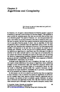
Equation 6 says that the extinction time for building blocks under random genetic drift alone grows linearly with the population size, and the constant factor decreases with the building block size. Table 1 shows the expected extinction time for building block sizes 1 through 5 using equation 6.

1200 k=1 k=2 k=3 k=4 k=5 1.386 N (k=1) 0.924 N (k=2) 0.594 N (k=3) 0.370 N (k=4) 0.224 N (k=5)

1000 generations to lose building block

(1969) showed that in a population of size N , the average number of generations to lose an allele that starts with a proportion p is

800

600

400

200

0 0

Drift time 1.386 N 0.924 N 0.594 N 0.370 N 0.224 N

Computer simulations of random genetic drift match the diffusion model quite well (see figure 1). 3.2

200

300

400

500

population size

Figure 1: Average time to lose a building block. The solid lines are from the diffusion model of Kimura and Ohta (1969). The isolated points were obtained by computer simulation. terminology is the same as the one adopted by the previous authors. The model assumes that when the most salient λ building blocks have converged, the remaining m − λ building blocks are still in their initial random state. The convergence model is based on the selection differential S(t), the difference between the mean fitness of the population at generation t + 1 and the population mean fitness at generation t. The selection intensity I(t) is the selection differential S(t) scaled by the standard deviation σ(t) of the population fitness: I(t) =

S(t) µ(t + 1) − µ(t) = σ(t) σ(t)

The increase in the population mean fitness from one generation to the next can be written as a function of λ:

Table 1: Expected extinction time for various building block sizes under the effect of random genetic drift. Building block size 1 2 3 4 5

100

I(t) =

µt+1 (λ) − µt (λ) σt (λ)

Next, we compute the mean and variance of the population fitness when λ building blocks have converged, but before doing that let’s compute the mean and variance of a single building block. In order to make the analysis simple, we consider that a k-bit building block correspond to a k-bit needle in a haystack (NIAH) function. In such a function, one solution has fitness fmax and the remaining 2k −1 solutions have fitness fmin . Let p = 1/2k , then the mean µ and variance σ 2 of a k-bit NIAH function is

DOMINO MODEL

This section applies the model developed by Thierens, Goldberg, and Pereira (1998) for building blocks. The

µ = p fmax + (1 − p) fmin 2

σ = p (fmax − µ)2 + (1 − p) (fmin − µ)2

In the case of our exponentially scaled problem, fmin = 0 and fmax is a power of 2 whose value depends on the building block’s salience (or importance). The mean and variance of the ith most salient building block is

µt+1 (λ) − µt (λ) = σt (λ) I Substituting the values for the mean µ(λ) and standard deviation σ(λ) obtained in equations 7 and 8, and simplifying gives

µbb(i) = p fmax = p 2m−i 2 σbb(i)

2

= p (1 − p) (fmax )

2−λt+1 = 2−λt

m−i 2

= p (1 − p) (2

)

We are now ready to calculate the mean and variance when λ building blocks have converged. Throughout the text, p = 1/2k denotes the expected proportion of building blocks in a uniformly random initialized population. The mean fitness µ(λ) is calculated by assuming that the first λ building blocks have already converged to the correct value, and the remaining m − λ building blocks are still in their initial random proportion.

λ X i=1

=

m X

2m−i +

p 2m−i

2j −

m−λ−1 X

j=0

2j + p

m−λ−1 X

j=0

2j

2−λt =

j=0

j=0 m−λ−1 X

− ln 2 ³ q ln 1 − I 3

4j

j=0

µ

p (1−p)

¶t

´ λt

− ln 2

ln 1 − I

p (1 − p) (2j )2

= p (1 − p)

p 3 (1 − p)

which is equivalent to

t=

For the variance calculation, it is only necessary to consider the non-converged region because the region that has already converged contributes nothing to the variance.

m−λ−1 X

µ r 1−I

(7)

= 2m − 1 + (p − 1)(2m−λ − 1)

σ 2 (λ) =

¶

Substituting p by 1/2k gives convergence time as a function of the building block size k:

i=λ+1

m−1 X

p 3 (1 − p)

When t = 0, λ0 = 0. Therefore

t=

µ(λ) =

µ r 1−I

(8)

4m−λ − 1 4−1 m−λ 4 ≈ p (1 − p) 3

= p (1 − p)

Thierens, Goldberg, and Pereira derived convergence times for both constant and variable selection intensities. Here, we limit ourselves to the case of constant selection intensities because they are the ones that yield faster convergence times. Examples of such selection schemes are tournament selection, truncation selection, and rankbased selection. In these schemes the average fitness increase from one generation to the next is equal to the product of the selection intensity I by the standard deviation of the population fitness:

√

3

¶ λt

(9)

√1

2k −1

Equation 9 says that the number of generations t until convergence is a linear function of the building block’s salience in the string. For example, for binary tour√ nament selection the selection intensity is I = 1/ π, and the expected number of generations until the entire string converges (λt = m) for the case of building blocks of size k = 1 is precisely the same equation that Thierens, Goldberg, and Pereira obtained: t=

³

− ln 2

ln 1 −

√1 3π

´ m = 1.76 m

As another example, for building blocks of size k = 3, the equation becomes t=

³

− ln 2

ln 1 −

√1 21π

´ m = 5.28 m

Just like in the original paper of Thierens, Goldberg, and Pereira, the constant factor obtained with the domino convergence model shouldn’t be taken too literally because this kind of modeling is not completely exact. Nevertheless, the functional form is correct (and is confirmed by experiments in section 3.4) and says that the average number of generations until convergence grows linearly with respect to the number of building blocks.

DOMINO AND DRIFT TOGETHER

By joining the drift model with the domino convergence model, it is possible to predict where in the string is the drift stall likely to occur. That’s precisely what we do next by equating the times for the two models, tdrif t ≈ tconvergence : 2 k ln 2 N≈ 2k − 1

− ln 2

µ ln 1 − I

¶ λ∗

1 √ √ 3 2k −1

N=2048 N=1024 N=512 N=256 N=128 N=64 N=32

200 generations to solve or lose BB

3.3

150

100

50

0

Rearranging gives:

0

20

40

60

80

100

120

140

160

180

200

BB number x

λ∗ ≈

2k

¶ √ 3

√1

2k −1

−1

N

(10)

Equation 10 says that given a population size N , it is possible to predict the number of building blocks λ∗ that will be solved correctly by the GA. Likewise, given a number of building blocks λ∗ that we wish to solve correctly, it is possible to predict the necessary population size needed by the GA to do so. Looking only at the functional form, equation 10 can be written as N = c λ∗ , where c is a constant that depends on the building block size k and the selection intensity I. The population size grows linearly with respect to the number of building blocks λ∗ . In section 3.2 we also observed that the average number of generations until convergence under the domino model is also a linear function of the number of building blocks. The number of fitness function evaluations taken by the GA is the product of the population size by the number of generations, and both are linear functions of the number of building blocks. Therefore, the overall time complexity of genetic algorithms on exponentially scaled problems, under the assumption of perfect mixing, is quadratic. The next section presents computer experiments that confirm a quadratic time complexity. 3.4

COMPUTER EXPERIMENTS

Computer experiments were performed on problems with 200 exponentially scaled building blocks. The experiments were done using binary tournament selection with replacement, and the building blocks mixed perfectly using a population-wise crossover operator similar to the one used in the compact GA (Harik, Lobo, & Goldberg, 1999) or UMDA (M¨ uhlenbein & Paaß, 1996). The experiments were done for building blocks of size 1 and 3. For size-1 building blocks, the population was initialized with exactly 50% ones and 50% zeros in each

Figure 2: Convergence behavior of an exponentially scaled problem with 200 building blocks of size k = 1 for various population sizes. 400 N=16384 N=8192 N=4096 N=2048 N=1024 N=512 N=256 N=128 N=64 N=32

350 generations to solve or lose BB

µ −2 k ln 1 − I

300 250 200 150 100 50 0 0

20

40

60

80

100

120

140

160

180

200

BB number x

Figure 3: Convergence behavior of an exponentially scaled problem with 200 building blocks of size k = 3 for various population sizes.

bit position. 100 independent runs were performed for population sizes 32, 64, 128, 256, 512, 1024, and 2048. Figure 2 plots the average number of generations needed to either solve or lose the building block for various population sizes. Building block number 0 is the most salient and building block number 199 is the least salient. The plot is identical to the one obtained by Thierens, Goldberg, and Pereira, except that in this case the results are shown for various population sizes. For very small population sizes the convergence process is largely dominated by the drift model, while for large population sizes the convergence is dictated by the domino model. For population sizes in the middle range, the most salient building blocks follow the domino model, and after some point, the drift effect starts to dominate.

Figure 3 is a similar plot for building blocks of size k = 3. Each building block is a NIAH function. The experiments were conducted in a similar way as the ones for k = 1, with the difference that in this case, the initial population had a proportion of 1/8 ones and 7/8 zeros (1/2k = 1/8, for k = 3). The experiments were done is this way to reflect an idealized building block mixing behavior. On an actual GA run, we should expect to observe slight differences from the results obtained in figures 2 and 3. Notice the straight lines obtained for the experiments with large population sizes in both figures 2 and 3. These results confirm the linear time complexity for run duration. The constant factor obtained from the theoretical model, however, is a conservative estimate. The difference between model and experiment can be explained due to the assumption that when the most salient λ building blocks have converged, the others are still in their initial random state. This is only an approximation of what actually happens in a GA run. There, when the λth building block has converged, the (λ + 1)th building block has already converged substantially, and is far from its initial random state. Therefore, on an actual GA run the convergence time is faster than the one predicted by the domino model. The experiments show a linear time complexity for run duration. In terms of population sizing, a look at the experimental data from our GA runs also reveals a linear growth. For example, in order to correctly solve the first 25 building blocks (in the case of k = 1) in at least 99% of the runs, the GA needed a population size of 256. To do the same thing for the first 50 building blocks a population size of 256 was not enough. Table 2 shows the population size needed to correctly solve the first 25, 50, 100, and 200 building blocks in at least 99% of the runs, for the case of size-1 building blocks. Table 3 shows the same thing for the case of size-3 building blocks. Table 2: Population size needed to correctly solve the first 25, 50, 100, and 200 size-1 building blocks in at least 99 out of 100 runs. Building blocks Population size 25 256 50 512 100 1024 200 2048 In both cases, when the number of building blocks doubles, the population sizing requirements also doubles. In summary, both population size and run duration grow linearly with the number of building blocks, giving an overall quadratic time complexity in terms of fitness function evaluations.

Table 3: Population size needed to correctly solve the first 25, 50, 100, and 200 size-3 building blocks in at least 99 out of 100 runs. Building blocks Population size 25 2048 50 4096 100 8192 200 16384

4

SUMMARY

This study extended the model of Thierens, Goldberg, and Pereira (1998) to analyze the time complexity of genetic algorithms on exponentially scaled problems. An extended drift and domino convergence model was presented along with computer simulations. The main result of this work is that under the assumption of perfect building block mixing, the overall time complexity of genetic algorithms on problems with exponentially scaled building blocks is a quadratic function of the number of building blocks.

5

CONCLUSIONS

For the two extreme cases of building block scaling, uniform and exponential, genetic algorithms with perfect mixing have time complexities of O(m) and O(m2 ) respectively. The linear time complexity for uniformly scaled problems occurs because the population sizing grows with the square root of m (Harik et al., 1999) and the time to convergence also grows with the square root of m (M¨ uhlenbein & Schlierkamp-Voosen, 1993). A quadratic time complexity for exponentially scaled problems does not seem that bad, and we may speculate that it diminishes the relevance of a fixed mutation operator as a means of introducing diversity in the population. Notice that a fixed mutation operator needs O(`k ) trials in order to discover a k-bit building block without messing up with the remaining parts of the problem (M¨ uhlenbein, 1992). The relevance of other building block diversity preservation techniques such as the one used in the Linkage Learning Genetic Algorithm (LLGA) (Harik, 1997) may also be not so important after all. The LLGA was able to solve exponentially scaled problems in almost linear time (Harik, 1997), (Lobo et al., 1998) due to a built-in probabilistic expression mechanism that preserved building block diversity and partly eliminated the problem of random genetic drift. Nevertheless, while the LLGA excelled in exponentially scaled problems, it did not do as well when solving other type of problems. The time complexity estimates presented herein are for

idealized situations because they assume perfect building block mixing. With traditional simple GAs, this assumption only occurs if the building blocks are trivial (size-1 building blocks), or when the user has knowledge about the structure of the problem (which is usually not true). However, with more advanced GAs that are able to learn gene linkage automatically, the assumption of perfect mixing is well approximated, and we should only expect to observe a slightly worse performance than in the idealized perfect mixing situation. The reason is that there may be a little overhead in population sizing and run duration needed by these advanced GAs in order to learn a problem’s structure, without which efficient building block mixing is not possible. Examples of such GAs are the Bayesian Optimization Algorithm (Pelikan, Goldberg, & Cant´ u-Paz, 1999) and the Extended Compact Genetic Algorithm (Harik, 1999). Acknowledgements This work was done while the first author was a visiting research scholar at the Illinois Genetic Algorithms Laboratory. Professor Goldberg’s contribution to this paper was sponsored by the Air Force Office of Scientific Research, Air Force Materiel Command, USAF, under grant F49620-97-1-0050. Research funding for this work was also provided by the National Science Foundation under grant DMI-9908252. Support was also provided by a grant from the U. S. Army Research Laboratory under the Federated Laboratory Program, Cooperative Agreement DAAL01-96-2-0003. The U. S. Government is authorized to reproduce and distribute reprints for Government purposes notwithstanding any copyright notation thereon. The views and conclusions contained herein are those of the authors and should not be interpreted as necessarily representing the official policies or endorsements, either expressed or implied, of the Air Force Office of Scientific Research, , the National Science Foundation, the U. S. Army, or the U. S. Government. References Asoh, H., & M¨ uhlenbein, H. (1994). On the mean convergence time of evolutionary algorithms without selection and mutation. In Davidor, Y., Schwefel, H.-P., & M¨ anner, R. (Eds.), Parallel Problem Solving from Nature, PPSN III (pp. 88–97). Berlin: Springer-Verlag. Crow, J. F., & Kimura, M. (1970). An introduction to population genetics theory. New York: Harper and Row. Goldberg, D. E., Deb, K., & Clark, J. H. (1992). Genetic algorithms, noise, and the sizing of populations. Complex Systems, 6 , 333–362. Goldberg, D. E., & Segrest, P. (1987). Finite Markov chain analysis of genetic algorithms. In Grefenstette, J. J.

(Ed.), Proceedings of the Second International Conference on Genetic Algorithms (pp. 1–8). Hillsdale, NJ: Lawrence Erlbaum Associates. Harik, G. R. (1997). Learning gene linkage to efficiently solve problems of bounded difficulty using genetic algorithms. Doctoral dissertation, University of Michigan, Ann Arbor. Also IlliGAL Report No. 97005. Harik, G. R. (1999). Linkage Learning via Probabilistic Modeling in the ECGA. (IlliGAL Report No. 99010). Urbana: University of Illinois at Urbana-Champaign, Illinois Genetic Algorithms Laboratory. Harik, G. R., Cant´ u-Paz, E., Goldberg, D. E., & Miller, B. L. (1999). The gambler’s ruin problem, genetic algorithms, and the sizing of populations. Evolutionary Computation, 7 (3), 231–253. Harik, G. R., Lobo, F. G., & Goldberg, D. E. (1999). The compact genetic algorithm. IEEE Transactions on Evolutionary Computation, 3 (4), 287–297. Hartl, D. L., & Clark, A. G. (1997). Principles of population genetics (3 ed.). Sunderland, Massachusetts: Sinauer Associates. Kimura, M. (1964). Diffusion models in population genetics. J. Appl. Prob., 1 , 177–232. Kimura, M., & Ohta, T. (1969). The average number of generations until fixation of a mutant gene in a finite population. Genetics, 61 , 763–771. Lobo, F. G., Deb, K., Goldberg, D. E., Harik, G. R., & Wang, L. (1998). Compressed introns in a linkage learning genetic algorithm. In Koza, J. R., Banzhaf, W., Chellapilla, K., Deb, K., Dorigo, M., Fogel, D. B., Garzon, M. H., Goldberg, D. E., Iba, H., & Riolo, R. L. (Eds.), Genetic Programming 98 (pp. 551–558). San Francisco: Morgan Kaufmann Publishers. M¨ uhlenbein, H. (1992). How genetic algorithms really work: I.Mutation and Hillclimbing. In M¨ anner, R., & Manderick, B. (Eds.), Parallel Problem Solving from Nature, 2 (pp. 15–25). Amsterdam, The Netherlands: Elsevier Science. M¨ uhlenbein, H., & Paaß, G. (1996). From recombination of genes to the estimation of distributions I. binary parameters. In Voigt, H.-M., Ebeling, W., Rechenberg, I., & Schwefel, H.-P. (Eds.), Parallel Problem Solving from Nature, PPSN IV (pp. 178–187). Berlin: Springer-Verlag. M¨ uhlenbein, H., & Schlierkamp-Voosen, D. (1993). Predictive models for the breeder genetic algorithm: I. Continuous parameter optimization. Evolutionary Computation, 1 (1), 25–49. Pelikan, M., Goldberg, D. E., & Cant´ u-Paz, E. (1999). BOA: the bayesian optimization algorithm. In Banzhaf, W., Daida, J., Eiben, A. E., Garzon, M. H., Honavar, V., Jakiela, M., & Smith, R. E. (Eds.), GECCO-99: Proceedings of the Genetic and Evolutionary Computation Conference (pp. 525–532). San Francisco, CA: Morgan Kaufmann. Thierens, D., Goldberg, D. E., & Pereira, A. (1998). Domino convergence, drift, and the temporal-salience structure of problems. In Proceedings of 1998 IEEE International Conference on Evolutionary Computation (pp. 535–540). Piscataway, NJ: IEEE.