Nov 10, 2009 - Finally, K (t,tâ²) is a memory kernel which describes the non-unitary effects of ..... the effective Hamiltonian ËHS +Vdis using the Suzuki-Trotter split operator ... C.A.R. thanks the Mary-Fieser Postdoctoral Fel- lowship program.
Time-Dependent Density Functional Theory for Open Quantum Systems with Unitary Propagation Joel Yuen-Zhou,1 David G. Tempel,2 César A. Rodríguez-Rosario,1 and Alán Aspuru-Guzik1 1 Department
of Chemistry and Chemical Biology, Harvard University, 12 Oxford Street, 02138, Cambridge, MA of Physics, Harvard University, 17 Oxford Street, 02138, Cambridge, MA
arXiv:0902.4505v3 [cond-mat.mtrl-sci] 10 Nov 2009
2 Department
We extend the Runge-Gross theorem for a very general class of Markovian and non-Markovian open quantum systems under weak assumptions about the nature of the bath and its coupling to the system. We show that for Kohn-Sham (KS) Time-Dependent Density Functional Theory, it is possible to rigorously include the effects of the environment within a bath functional in the KS potential, thus placing the interactions between the particles of the system and the coupling to the environment on the same footing. A Markovian bath functional inspired by the theory of nonlinear Schrödinger equations is suggested, which can be readily implemented in currently existing real-time codes. Finally, calculations on a helium model system are presented. PACS numbers: 31.15ec,71.15Mb,02.70.-c,71.15.-m,31.10+z
Current advances in the manipulation and control of nanoscale systems allow for an unprecedented opportunity to probe the non-equilibrium dynamics of a wide variety of condensed matter systems on a broad range of timescales [1, 2, 3]. Serious effort is therefore required for the development of tractable theoretical methods that can shed some light on many-body dynamics without directly solving the timedependent Schrödinger equation (TDSE) for an object composed of many particles. One of the most promising methods in this regard is Time-Dependent Density Functional Theory (TD-DFT) [4, 5, 6], which is formally equivalent to the TDSE, but is based on the particle density rather than the wavefunction. Recently, there has been a considerable interest in developing an Open Quantum Systems (OQS) formalism for TDDFT, where the number of particles in the system remains fixed, but there is energy exchange with an environment [7, 8, 9, 10, 11, 12, 13]. This effort allows for the description of particle transfer within the system, spontaneous decay, inelastic scattering, and many other ubiquitous relaxation and dephasing phenomena. For a Markovian equation of the Lindblad form, Burke, Car, and Gebauer (BCG) proved that a statement analogous to the Runge-Gross (RG) theorem holds, namely, that there is a one-to-one correspondence between the time-dependent particle density and the external scalar potential provided that the particle-particle interaction, initial quantum state, and the bath jump-operators remain fixed [7]. To place their result in a practical context, BCG assumed the existence of a Kohn-Sham (KS) scheme in order to carry out their calculations. In the mentioned procedure, an artificial noninteracting open system, the so-called KS system, evolves under an effective KS potential and is expected to reproduce the particle density of the original system [14]. By virtue of their theorem, any observable is a functional of the particle density, so in principle, the KS system contains all the information about the observables of the original system. The question of whether or not such a non-interacting KS system exists is not obvious, but clearly crucial for KS theory, and it is known as the non-interacting V-representability problem [15, 16]. We note that non-interacting V-representability in the context of BCG’s formalism has been assumed, but not formally proven.
In the case of closed systems, Van Leeuwen has proved that it is in fact possible to reproduce the particle density of a many-body interacting system with an effective KS potential acting on an auxiliary system with no particle-particle interactions [15]. This KS potential is unique, and in general, expected to show a nonlinear and nonlocal funcional dependence on the history of the particle density [17]. Intuitively, we can argue that in the KS system we formally give up the linearity of the many-body equation of motion for a nonlinear surrogate which, nevertheless, is an effective single-particle equation. With this in mind, a natural question to ask is: Just as with the particle-particle interactions, can we subsume the coupling between the system and the bath into an additional nonlinearity of the density in the effective KS potential? In the next paragraphs, we report that this is indeed the case. Consider an N-particle open quantum system described by a time-dependent density matrix ρ (t) which, in the position representation, is a function of 6N coordinates and time t. The most general equation of motion for an open quantum system is a master equation of the form (atomic units used throughout) [18],
ˆ ρ˙ (t) = −i[H(t), ρ (t)] + |~pˆi |2 2m
Zt 0
K (t,t ′ )ρ (t ′ )dt ′ + T (t).
(1)
i + V (~rˆi ,t) + ∑i< j U(~rˆi ,~rˆ j ) is the genˆ erator of the unitary piece of the evolution. In general, H(t) is an effective renormalized Hamiltonian of the system due to its interaction with the bath, where U(~ri ,~r j ) is a symmetric pairwise interaction potential and V (~r,t) an external scalar potential. Finally, K (t,t ′ ) is a memory kernel which describes the non-unitary effects of the bath on the evolution of the system, and T (t) is an inhomogeneous term which is present only if there are initial correlations between the system and the bath. Quite generally, K (t,t ′ ) and T (t) may be functions of V (~r,t), such as in the case of a strong laser field interacting with a molecule in condensed phase [19], whereas T (t) may also depend on the initial state ρ (0). Furthermore, for notation, we define the operators that measure the particle density as n(~ ˆ r) = ∑i δ (~r −~rˆi ) and the current ˆ Here, H(t) = ∑i
h
2 ˆ r) = density as ~j(~ state a theorem.
1 2
∑i {δ (~r − rˆi ), vˆi }. We are now ready to
Theorem.- Let the original system be described by the density matrix ρ (t) which, starting as ρ (0), evolves according to Eq. (1). Consider an auxiliary system associated with the density matrix ρ ′ (t) and initial state ρ ′ (0), which is governed by the equation:
ρ˙ ′ (t) = −i[Hˆ ′ (t), ρ ′ (t)] +
Z t 0
dt ′ K ′ (t,t ′ )ρ ′ (t ′ ) + T ′ (t), (2)
where the functional forms of K ′ (t) andh T ′ (t) are given, i pˆ i |2 and its Hamiltonian reads as Hˆ ′ (t) = ∑i |~2m + V ′ (~rˆi ,t) + ∑i< j U ′ (~rˆi ,~rˆ j ), where U ′ (~ri ,~r j ) is also given. Under mild conditions, there exists an external potential V ′ (~r,t) that drives the auxiliary system in such a way that the particle densities in the original and the auxiliary systems are the same at every point in time and space, i.e., hn(~ ˆ r)it′ = hn(~ ˆ r)it . This statement is ′ ′ ˆ r)it=0 = hn(~ ˆ r)it=0 true provided that ρ (0) guarantees that hn(~ ′ ˙ ˙ and hn(~ ˆ r)it=0 = hn(~ ˆ r)it=0 .
Proof.- We use similar techniques to the ones employed by van Leeuwen [15] and Vignale [16]. The detailed steps of a related derivation may be found in [20]. First, by using Eq. (1), we can find the equation of motion for the second derivative of the particle density of the original system with respect to time: ~ r,t) + ¨ˆ r)it = ~∇ · [hn(~ hn(~ ˆ r)it ~∇V (~r,t)/m + D(~ ~ (~r,t)/m + G~ (~r,t)] + J (~r,t). F
(3)
Here, ~∇V (~r,t) is proportional D to the external electric E ~ r,t) = − 1 ∑α ,β βˆ ∂ ∑i {vˆiα , {vˆiβ , δ (~r −~rˆi )}} is field, D(~ 4 ∂α the divergence of the stress tensor, where α , β = x, y, z, ~ (~r,t) is the internal force density caused by the pairF ~ (~r,t) = −h∑i δ (~r − ~rˆi ) ∑ j6=i ~∇~r U(~ri −~r j )i, wise potential F i ˆ r)(R t dt ′ K (t,t ′ )ρ (t ′ ) + T (t))} and and G~ (~r,t) = Tr{~j(~ � R 0 J (~r,t) = ∂∂t Tr{n(~ ˆ r) 0t dt ′ K (t,t ′ )ρ (t ′ ) + T (t) } are terms which arise due to the coupling to the bath. Similarly, by employing Eq. (2), it is possible to derive an equivalent equa¨ˆ r)it′ , where the variables in Eq. (3) are substituted tion for hn(~ by their primed analogues. If we subtract these two equations and eliminate the variable hn(~ ˆ r,t)i′ with the restriction ′ hn(~ ˆ r)it = hn(~ ˆ r)it , we obtain an identity with time-dependent parameters that can be Taylor expanded about t = 0. Denotk r,t) |t=0 , ing the Taylor expansion coefficients by Ok ≡ k!1 ∂ O(~ ∂ tk l we collect the terms of order t , and arrive at the expression:
−~∇ · (n0 (~r)~∇(Vl′ (~r))) = ~ ′ (~r) + F ~ ′ (~r) + mG~ ′ (~r)) + mJ ′ (~r) −~∇ · (mD l l l l ~ l (~r) + F ~ l (~r) + mG~ l (~r)) − mJ l (~r) +~∇ · (mD ! l ′ −~∇ · (n0 (~r)~∇(V l (~r))) + ~∇ · ∑ nk (~r)~∇(Vl−k − V l−k (~r)) . k=1
(4) We now make a claim: If the right hand side of Eq. (4) contains no coefficients Vk′ (~r) for k ≥ l, it can be regarded as a recursion relation to construct Vl′ from the lower order coefficients Vk′ (~r) for 0 ≤ k < l. This would imply that each coefficient can be uniquely solved recursively upon the specification of a boundary condition, which we can conveniently set to Vl′ (~r) → 0 as |~r| → ∞, for all l. Finally, the explicit construction of V ′ (~r,t) through its Taylor coefficients, V ′ (~r,t) = ∑k Vk′ (~r)t k , proves the theorem. If K ′ (t,t ′ ) and T ′ (t) do not depend explicitly on V ′ (~r,t), the claim can be systematically shown [20]. Otherwise, l ′ ′ Jl′ (~r) can depend at most on K ′t=t ≡ l!1 ∂ K∂ t l(t,t) |t=0 (the l R integral terms 0t dt(·) naturally vanish at t = 0) and Tl ′ = 1 ∂ l T ′ (t) l! ∂ t l |t=0 .
General expressions derived with projectionoperator methods [19] can be used to formally show that ′ ′ K ′ t=t should depend at most on Vl−1 (~r), which supports our l claim. This fact can be interpreted in very physical terms: the action of the external field V ′ (~r,t) on the system is local in time through the unitary piece of the master equation. The effects of V ′ (~r,t) on the system leak out to the bath and return as memory effects through the memory kernel only at times t ′′ strictly later than t. In other words, K ′ (t,t) can depend on V ′ (~r,t ′ ) for t ′ < t, but should not depend on the instantaneous V ′ (~r,t). A similar conclusion may not be made for arbitrary Tl ′ terms, since at t = 0, the initial correlations between the system and the bath may depend on V (~r, 0), and Tl ′ could depend on Vl′ (~r). However, as long as Tl ′ depends at most on ′ (~r), the claim and the theorem will necessarily hold. This Vl−1 is the only warning of the proof, and this requirement can be checked on a case by case basis, but it is easily guaranteed in the case of initial factorizable conditions between the system and the bath, or if the inhomogeneity is V -independent, which occurs if the external field is weak or if the bath is Markovian. � Several important corollaries hold from the theorem. If ρ ′ (0) = ρ (0), U ′ (~ri ,~r j ) = U(~ri ,~r j ), K ′ (t,t ′ ) = K (t,t ′ ), and ′ −V T ′ (t) = T (t), then Eq. (4) reads: −~∇ · (n0~∇(Vl−k l−k )) = � � l ′ ′ ~∇· ∑ nk~∇(V − V l−k ) , which means that V = Vl for all k=1
l−k
l
l. This allows for an extension of the RG theorem to a large class of OQS: For fixed initial state, interparticle potential, memory kernel and inhomogeneity, there is a one to one map between particle densities and scalar potentials. This statement allows us to regard the time-dependent particle density
3 as a fundamental variable just as the time-dependent density matrix. For Markovian equations of the Lindblad form, this reduces to the result proven by GCB. The theorem also justifies the KS scheme of BCG and its generalization to a wide range of OQS, namely, that it is possible to choose an auxiliary open system with no particleparticle interactions, U ′ (~ri ,~r j ) = 0, to reproduce the same particle density as the original system. However, we want to take a different approach on the subject and make the observation that the proof also allows us to consider the case where U ′ (~ri ,~r j ) = K ′ (t,t ′ ) = T ′ (t) = 0, that is, a KS system that evolves unitarily as if it were a driven closed system, but still reproduces the particle density of the original open system that interacts with the bath and evolves through a non-unitary equation of motion. Therefore, we have rigorously justified the intuition hinted at the beginning of the letter, that is, the possibility to conceive of a KS system where we subsume the effects of the bath in an additional term in the KS potential [29]. In this new KS theory, we shall rewrite the KS potential as V ′ = V + VH + Vxc + Vbath , where V is the original exterR hn(~ ˆ r′ )i nal potential, VH (~r,t) = d 3 r′ |~r−~r′ |t is the Hartree term, Vxc is a standard approximation to the exchange-correlation (xc) term due to the many-body effects within the system, such as an adiabatic functional [21], and finally, Vbath is the new term due to the bath, which includes additional correlations on the particles of the system, and which we expect to be nonadiabatic. Finally, we must discuss the feasability of the initial conditions for our KS scheme. It is always possible to propose a pure state single Slater determinant ψ˜ ′ (0) = √1N! det[φi (~r j )] which satisfies the restriction hψ˜ ′ (0)|n(~ ˆ r)|ψ˜ ′ (0)i = hn(~ ˆ r)it=0 by employing the Harriman construction [22]. By defining a new state ψ ′ (0) = √1N! det[φi (~r j )eiαi (~r j ) ], the set of phases {αi } can be chosen with considerable freeˆ r)|ψ ′ (t)i|t=0 = −~∇ · dom in order to satisfy ∂∂t hψ ′ (t)|n(~ � � ˙ˆ r)it=0 , in which ∑i |φi (~r)|2~∇(−i arg(φi (~r) + αi (~r)) = hn(~ case, we can choose ψ ′ (0) as the initial KS wavefunction, or equivalently, ρ ′ (0) = |ψ ′ (0)ihψ ′ (0)| as the initial KS density matrix. Note that this argument is irrespective of the purity of the initial state of the original system. Model system and suggestion of “bath” functional.- We refer the reader to Ref. [20], which reports a numerical study that constructs the KS potential V ′ for a harmonic oscillator model coupled to a heat bath. In this letter, we will be concerned with the study of a model system, namely, a 1d helium atom [23, 24] coupled to a heat bath. We write the total system-bath Hamiltonian as HT = HS + HSB + HB . � HS = ∑2i=1 Pi2 /2 + V(Xi ,t) + W (X1 − X2 ) describes the helium atom, with Xi and Pi denoting √ the positions and momenta of the electrons, W (X) = e2 / X 2 + 1 being a softCoulomb potential, and V (X) = −2W (X) the external potential, which is only due to # the nucleus. HB + HSB = " in this case �2 � c j 1 2 2 corresponds to a har2 ∑ j m j x˙ j + ∑i ω j x j − m ω 2 Xi j
j
monic bath with bilinear coupling to the positions of the elec-
trons. We assume that the bath is an infinite set and its distribution of couplings can be approximated by a continuous Ohmic spectral density, J(ω ) = ∑ j
θ (ω ) ξ20 ω e−ω /ωc ,
c2j 2m j ω j δ (ω j
− ω) =
where θ (ω ) is the step function, ξ0 is the intensity of the coupling, and ωc is a cutoff frequency for the bath modes. From a computational point of view, the dynamics of the composite system-bath object is intractable. Since the emphasis is on the system, and not on the bath, we take an OQS approach: For weak coupling ξ0 and large ωc , the BornMarkov approximation is justified, and it is straightforward to obtain a memoryless master equation of the Lindblad form for the system. At zero temperature (T = 0), it reads,
γ ρ˙ (t) = −i[H˜ S , ρ ] − (L† Lρ + ρ L† L − 2Lρ L† ), 2
(5)
where H˜ S = HS + ξ02ωc (x2 + y2 ) is a renormalized Hamiltonian due to coupling to the bath. We denote |gi and |ei to be the ground and first singlet excited states of H˜ S respectively, so that the jump operators L can be expressed in the form L = |gihe|. L promotes quantum jumps from |ei to |gi. The rate of these transitions is captured by γ = 2π |he|µ |gi|2J(ωeg ), where µ = ∑2i=1 Xi is the dipole operator. We proceed to derive a bath functional which could be used in the KS theory for TD-DFT applied to systems interacting with a Markovian bath, just like our model system. For a single particle, Kostin [25] has previously constructed a dissipative nonlinear Schrödinger equation, where i ∂∂ψt = H ψ , for which the Hamiltonian in 1-D reads H =
p2 2M
+V +V � �bath, with
λ . ln ψψ∗(X,t) the bath potential being given by Vbath (X,t) = 2i (X,t) This equation of motion has the very interesting property that at the level of observables, it satisfies the Langevin ˙ = hPi , hPi ˙ = −λ hPi − h ∂ V (Z,t) i, equation at T = 0, i.e., hXi M ∂Z as can easily be checked by direct substitution. The friction coefficient λ may be obtained from a microscopic derivation of the Langevin equation, which in the case of a particle bilinearly coupled to an Ohmic bath of strength ξ0 , yields λ = πξ0 /2. Furthermore, a quick inspection allows us to rewrite Vbath as a functional of the particle density [30],
ˆ ′ )it ](X,t) = λ Vbath [hn(X ˆ ′ )it , h j(X
Z X
−∞
dX ′
ˆ ′ )it h j(X . hn(X ˆ ′ )it
(6)
For more than one particle, this identification is not formally possible, but regardless, we shall heuristically assume it as our Markovian bath functional (MBF) [31]. Non-Markovian generalizations of Eq. (6) may be readily conceived starting from nonlinear Schrödinger equations which reproduce the generalized Langevin equation for its observables. Physically, this suggestion is very appealing: The dragging force due to the jˆ(X)it , which is the velocity field. The MBF is proportional to hhn(X)i ˆ t coefficient λ can be approximated from the spectral density and conveniently scaled to reflect the many-body coupling to
4 the bath. From the single Slater determinant KS wavefunction, ψKS (t) = √1N! det[φi (X j ,t)], we can express Vbath (X,t) = Rz c
,t)| ∇αi (X ,t) , where αi = −i arg(φi ). dX ′ ∑i |φi (X ∑ |φ (x,t)|2 ′
i
2
′
2
i
In order to gain insight on the system of consideration, we performed several calculations for which the results are summarized in Fig. 1. The initial state of the helium atom was taken to be the pure state ψ (0) = √12 (|gi + |ei). We propagated the system in real time with three different methods. For the first method (black solid curve), we evolved the density matrix of helium using the master Eq. (5). We chose a spectral density with values ξ0 = 0.01 Eh and ωc = 10 Eh. The real space eigenbasis of H˜ S was obtained with the OCTOPUS package [26], resulting on an energy gap ∆eg = 0.85 Eh and a dipole moment he|µ |gi = 1.1 a.u. The choice of parameters justifies the Markovian conditions for the master equation. The expected damped oscillations calculated with this method are shown in the solid curve. The second method (red solid curve) was performed to calibrate the parameter λ in Vdis . We evolved the time dependent Schrödinger equation with the effective Hamiltonian H˜ S + Vdis using the Suzuki-Trotter split operator method [27], where the many-body dynamics was computed exactly via H˜ S , but the coupling to the bath entered through the nonlinear dependence of Vdis on hn(~ ˆ r)it . We scanned several λ parameters and found λ = 0.075 Eh to reproduce the curve derived from (A) with high accuracy [32]. Finally, for the third method (black dotted curve) we carried out a TD-DFT KS calculation with exact exchange and same dissipation rate γ as in B, that is, VKS = 21 VH + Vdis , R ˆ ′ )it . The result for this last with VH (X,t) = γ dX ′ √ hn(X ′ 2 1+(X−X )
method yields poor results with unphysical Rabi-like oscillations. The latter are caused by the absence of correlations caused by particle-particle interactions [28]. Nevertheless, the oscillations decay on a similar timescale to the other calculations, and reach a steady state due to the MBF.
In summary, we have formally extended TD-DFT to a large class of OQS, and rigurously showed the possibility of including the effects of the bath on the dynamics of the system within a bath functional. The latter enters into a TD-DFT calculation on the same footing as the standard exchangecorrelation functionals exclusively due to many-body dynamics. We have suggested Eq. (6) as the Markovian bath functional which can be readily implemented in currently existing TD-DFT codes. Future work must address the derivation of the friction coefficient λ from a more systematic procedure, the explicit derivation of bath functionals for more complex memory kernels, and finally, the role of fluctuations and finite temperatures in this unitary propagation KS formalism. Stimulating discussions with many members of the AspuruGuzik group are greatly acknowledged. J.Y.Z. also thanks the generous support of Fundación México at Harvard and CONACYT. C.A.R. thanks the Mary-Fieser Postdoctoral Fellowship program. This work was carried out under the DARPA contract FA 9550-08-1-0285.
1.5 1
Dipole (a.u.)
λ
2.5
0.5 0 −0.5 −1 −1.5 −2
0
50
100
150
Time (a.u.)
(a) FIG. 1. Evolution of the dipole moment of a helium atom coupled to a heat bath. We present three different calculations: The black solid curve represents the "exact" calculation using a master equation. The red solid curve is the propagation of the exact many-body dynamics of helium plus the MBF. Finally, the dotted black is the TD-DFT calculation with exact exchange and MBF. The last calculation yields poor results due to the absence of correlations in the electron interactions. Details of the calculations can be found in the text.
[1] M. F. Hawthorne, J. I. Zink, J. M. Skelton, M. J. Bayer, C. Liu, E. Livshits, R. Baer, and D. Neuhauser, Science 303, 1849 (2004). [2] A. Troisi, J. M. Beebe, L. B. Picraux, R. D. van Zee, D. R. Stewart, M. A. Ratner, and J. G. Kushmerick, Proc. Natl. Acad. Sci. U.S.A. 104, 14255 (2007). [3] E. Goulielmakis, M. Schultze, M. Hofstetter, V. S. Yakovlev, J. Gagnon, M. Uiberacker, A. L. Aquila, E. M. Gullikson, D. T. Attwood, R. Kienberger, et al., Science 320, 1614 (2008). [4] E. Runge and E. K. U. Gross, Phys. Rev. Lett. 52, 997 (1984). [5] K. Burke, J. Werschnik, and E. K. U. Gross, J. Chem. Phys. 123, 062206 (2005). [6] M. A. L. Marques and E. K. U. Gross, Ann. Rev. Phys. Chem. 55, 427 (2004). [7] K. Burke, R. Car, and R. Gebauer, Phys. Rev. Lett. 94, 146803 (2005). [8] M. Di Ventra and R. D’Agosta, Phys. Rev. Lett. 98, 226403 (2007). [9] M. Koentopp, C. Chang, K. Burke, and R. Car, J. Phys. Condens. Matter 20, 083203 (2008). [10] C. A. Ullrich and G. Vignale, Phys. Rev. Lett. 87, 037402 (2001). [11] S. Piccinin and R. Gebauer, ChemPhysChem 6, 1727 (2005). [12] R. D’Agosta and G. Vignale, Phys. Rev. Lett. 96, 016405 (2006). [13] X. Zheng, F. Wang, C. Y. Yam, Y. Mo, and G. Chen, Phys. Rev. B 75, 195127 (2007). [14] W. Kohn and L. J. Sham, Phys. Rev. 140, A1133 (1965). [15] R. van Leeuwen, Phys. Rev. Lett. 82, 3863 (1999). [16] G. Vignale, Phys. Rev. B 70, 201102 (2004). [17] N. T. Maitra, K. Burke, and C. Woodward, Phys. Rev. Lett. 89, 023002 (2002).
5 [18] H.-P. Breuer and F. Petruccione, The theory of open quantum systems (Oxford University Press, 2002). [19] C. Meier and D. J. Tannor, J. Chem. Phys. 111, 3365 (1999). [20] J. Yuen-Zhou, C. Rodriguez-Rosario, and A. Aspuru-Guzik, Phys. Chem. Chem. Phys. 11, 4509 (2009). [21] R. Baer, J. Mol. Struct. 914, 19 (2009). [22] J. E. Harriman, Phys. Rev. A 24, 680 (1981). [23] M. Thiele, E. K. U. Gross, and S. Kummel, Phys. Rev. Lett. 100, 153004 (2008). [24] C. Harabati and K. G. Kay, J. Chem. Phys. 127, 084104 (2007). [25] M. D. Kostin, J. Chem. Phys. 57, 3589 (1972). [26] M. Marques, A. Castro, G. Bertsch, and A. Rubio, Comp. Phys. Chem. 151, 60 (2003). [27] R. Kosloff, J. Phys. Chem. 92, 2087 (1988). [28] M. Ruggenthaler and D. Bauer, Phys. Rev. Lett. 102, 233001 (2009). [29] We clarify that other observables besides the particle density many not be the same in the driven closed KS system when compared to the ones corresponding to the open original system. On the other hand, due to the RG-like statement we have derived, any observable is a functional of the particle density,
which is in principle the same in both original and KS systems. [30] In 1-d, we can express the current as a functional of the partiR z ∂ hn(z ˆ ′ )i ′ ˆ t = − −∞ cle density, h j(z)i ∂ t dz , where we have assumed ˆ h j(±∞)i = 0. For more dimensions, this might not be possible, as we will explain, this is not a problem from a practical perspective in the KS propagation. [31] Eq. (6) will not be able to cause transitions from eigenstates, ˆ ′ )it = 0. For these cases, the inwhich have the property h j(X clusion of a small penalty functional κ (hn(X)i ˆ ˆ t − hn(X)i target ) to Vbath guarantees the proper evolution of the KS system. Here, | λκ | a10 ≪ 1, and hn(X)i ˆ target represents the final steady state particle density, [32] From a microscopic derivation, it is possible to argue that an approximate friction coefficient arising from the coupling of the 0π bath to two electronic coordinates could be λ ≈ ξ√ = 0.01 Eh , 2 2 which differs from the optimized value. The difference between these two values may be due to the lack of dependence of λ on ωc . A more systematic derivation of λ and a detailed examination of this problem will be addressed in future work.