Time development in quantum mechanics using a reduced Hilbert space approach M. Bellonia兲 and W. Christianb兲 Physics Department, Davidson College, Davidson, North Carolina 28035
共Received 3 September 2007; accepted 6 January 2008兲 We have created a suite of open source programs that numerically calculate and visualize the evolution of arbitrary initial quantum-mechanical bound states. The calculations are based on the expansion of an arbitrary wave function in terms of basis vectors in a reduced Hilbert space. The approach is stable, fast, and accurate at depicting the long-time dependence of complicated bound states. Several real-time visualizations, such as the position and momentum expectation values and the Wigner quasiprobability distribution for the position and momentum, can be shown. We use these computational tools to study the time-dependent properties of quantum-mechanical systems and discuss the effectiveness of the algorithm. © 2008 American Association of Physics Teachers. 关DOI: 10.1119/1.2837810兴 I. INTRODUCTION Wave packets, localized solutions of the Schrödinger equation, have been of interest since the beginning of quantum mechanics. It was Schrödinger1 who first proposed a localized solution 共a wave packet兲 to his wave equation as a way to study the connections between classical and quantum mechanics. Others soon found explicit wave packet solutions for localized quantum-mechanical “particles” subject to no force2 共constant velocity兲 and a constant force3 共constant acceleration兲, respectively. For a variety of reasons 共such as the lack of computational power and lack of experimental verification兲, the study of wave packets lay dormant for many years. However, over the last 30 years quantum-mechanical wave packets and their revivals 共the property that certain bound-state wave packets reform to their original shape in a predictable way兲 have received much theoretical attention and experimental verification.4 In addition, quantum chaos5 has emerged as a way to study quantum-mechanical systems whose classical counterparts exhibit chaos 共even though the quantum-mechanical systems do not兲. Many of these recent theoretical studies have focused on the long-time behavior of wave packets by utilizing specialized visualizations, such as the quantum carpet,6 the Wigner distribution,7 and, for quantum chaos, the Hussimi distribution.8 These calculations and visualizations are often generated using a symbolic mathematical manipulation program to construct, evolve, and visualize energy eigenstates and their linear superpositions. Although numerous computer programs and algorithms exist for the accurate numerical determination of energy eigenfunctions and eigenvalues,9,10 the long-time evolution of arbitrary initial states is particularly difficult for positionspace or momentum-space numerical algorithms to handle. To attain the necessary accuracy the spatial grid and the time steps used must be very small, and hence it takes many computations to reach the revival time scale. As a result, numerical errors accumulate and, although the algorithms are stable because they conserve probability, they cease to be accurate enough to show important long-time features of the quantum-mechanical state. To address these issues we have developed a suite of opensource simulations as part of the Open Source Physics Project.11 These programs simulate the time evolution based on the expansion of an arbitrary wave function in terms of 385
Am. J. Phys. 76 共4&5兲, April/May 2008
the basis vectors in a reduced Hilbert space.12 Because the programs are based on the superposition principle, many of the drawbacks we have described of standard numerical algorithms do not arise, allowing for the visualization of wave packets. The programs make the creation and study of quantum-mechanical superpositions easy and accessible for students and instructors. II. REVIEW OF TIME-EVOLUTION ALGORITHMS The time-dependent quantum mechanical wave function is inherently complex 共here in one dimension and in position space兲:
冋
−
册
ប2 2 2 + V共x兲 ⌿共x,t兲 = iប ⌿共x,t兲. t 2m x
共1兲
The evolution of an arbitrary state is given by ˆ
⌿共x,t兲 = e−iH共t−t0兲/ប⌿共x,t0兲, ប2
共2兲
2
ˆ =− where the operator H 2m x2 + V共x兲 is the Hamiltonian. To solve Eq. 共1兲 for an arbitrary potential energy function, we first specify the wave function ⌿共x , t0兲 at some initial time t0 and then evolve it in time as ˆ
⌿共x,t0 + ⌬t兲 = e−iH共⌬t兲/ប⌿共x,t0兲,
共3兲
where ⌬t is the time step. Standard approaches such as Crank–Nicolson,13 Numerov,14 split operator, and staggered-time 共also called half-step兲,15 accomplish this update in a variety of ways.16 These algorithms are successful since they are inherently stable since they conserve probability and energy. However, for long times numerical errors begin to accumulate and the results will eventually deviate from the “true” results. The accumulation of errors is most often found in the inaccurate depiction of the shape of the wave function and the phase. Such inaccuracies can mask the often subtle long-time features of quantum-mechanical systems and limit these algorithms to the study of short times. III. THE REDUCED HILBERT SPACE APPROACH In the reduced Hilbert space approach,17 more generally called the spectral method,18 the basis set of Hilbert space,
http://aapt.org/ajp
© 2008 American Association of Physics Teachers
385
which is typically an infinite dimensional space, is limited to some finite dimension N. As a practical matter we rarely construct a complete Hilbert space, and such a construction is often impractical or impossible. Because of finite computer resources, we cannot create an infinite number of basis vectors to represent a complete Hilbert space, but for many problems it suffices to have a reduced Hilbert space. To see how this reduction will 共or won’t兲 affect the end result, we construct two projection operators, N
ˆ = 兺 兩 典具 兩 P N n n
共4兲
n=1
and ⬁
ˆ = P D
兺
兩n典具n兩,
= 兺 e−iEnt/ប兩n共0兲典具n共0兲兩⌿共0兲典,
共12b兲
n=1
Hence, 兩⌿N共t兲典 where cn ⬅ 具n共0兲 兩 ⌿共0兲典. N −iEnt/ប = 兺n=1cne 兩 n共0兲典. The construction of a linear superposition in position space using the reduced Hilbert space approach proceeds like the usual case for a linear superposition of energy eigenstates as long as we satisfy two conditions: 共1兲 the Hilbert space is large enough so that a finite subset of basis states is sufficient to properly represent the initial state and 共2兲 we have accurate energy eigenfunctions n共x兲 and energy eigenvalues En corresponding to the potential energy function V共x兲. Energy eigenfunctions and eigenvalues can be computed using a numerical algorithm if analytic expressions are unavailable.
共5兲
n=N+1
IV. PROGRAM DESCRIPTION
where the sum of the two projection operators in Eqs. 共4兲 and ˆ . We consider an 共5兲 is the complete projection operator, P arbitrary initial state 兩⌿典 and define ˆ 兩⌿典 and 兩⌿ 典 ⬅ P ˆ 兩⌿典, 兩⌿N典 ⬅ P N D D
共6兲
which describes the part of the original wave function that is in the reduced Hilbert space and the part that is not. We can write ˆ 兲共P ˆ +P ˆ 兲兩⌿典 ˆ 兩⌿典 = H ˆ 共P ˆ +P H N D N D ˆP ˆ 兩⌿ 典 + H ˆP ˆ 兩⌿ 典, =H N N D D
共7a兲 共7b兲
ˆ =P ˆ = Iˆ and P ˆ 兩⌿ 典=P ˆ 兩 ⌿ 典 = 0. ˆ +P because P N D N D D N We now construct the complete Schrödinger equation for ˆ and P ˆ on Eq. 共1兲 using Eq. 兩⌿D典 and 兩⌿N典 by operating P N D 共7b兲:
ˆ ˆ ˆ ˆ ˆ ˆ H P N PN兩⌿N典 + PNHPD兩⌿D典 = iប 兩⌿N典 t
共8兲
ˆ ˆ ˆ ˆ ˆ ˆ H P D PN兩⌿N典 + PDHPD兩⌿D典 = iប 兩⌿D典. t
共9兲
and
If in our computations 共by virtue of the state, 兩⌿典 selected兲, 兩⌿D典 is vanishingly small, then we are left with
ˆ ˆ ˆ H P N PN兩⌿N典 = iប 兩⌿N典, t
共10兲
which when integrated yields ˆ
ˆ ˆ
兩⌿N共t兲典 = e−iPNHPNt/ប兩⌿N共0兲典.
共11兲
If we can compute a precise subset of energy eigenvectors 兵n其, 关H , PN兴 = 0, because the projection operator is constructed from these energy eigenvectors. Equation 共11兲 then simplifies to ˆ
ˆ
ˆ 兩⌿共0兲典 兩⌿N共t兲典 = e−iHt/ប兩⌿N共0兲典 = e−iHt/បP N 386
N
Am. J. Phys., Vol. 76, Nos. 4 & 5, April/May 2008
共12a兲
The QMSUPERPOSITION program solves Eq. 共1兲 by first creating a table of energy eigenfunctions and eigenvalues of the time-independent Schrödinger equation in position space 共using units where ប = 2m = 1兲, and then creating linear superpositions of such states. Because the infinite square well, simple harmonic oscillator, and infinite well with periodic boundary conditions are standard problems with well-known analytic solutions, the energy eigenfunctions and eigenvalues associated with these potential energy functions are coded into the program. If an arbitrary potential energy function is chosen, the program determines the energy eigenfunctions and eigenvalues via the shooting method with hard 共infinite兲 walls at the positions xmin and xmax. As shown in Fig. 1 and in more detail in Table I, the QMSUPERPOSITION program allows the user to change several input parameters. For example, in the V共x兲 dialog box well, sho, or ring can be chosen, and the program will use the analytic energy eigenfunctions and eigenvalues for the infinite square well, the harmonic oscillator, or the infinite well with periodic boundary conditions, respectively. For any user-defined potential energy function, the program will calculate the energy eigenfunctions and eigenvalues numerically. For example, an asymmetric infinite square well can be simulated by setting xmin= −3, xmax= 3, and V共x兲 = 100 * step共x兲, where step共x兲 denotes the Heaviside step function, 共x兲. A superposition is then constructed based on the real and imaginary components of the expansion coefficients, cn, which the user supplies in a comma-delimited list, Re兵cn其 = 兵a1,a2,a3,a4, . . . ,aN其
共13a兲
Im兵cn其 = 兵b1,b2,b3,b4, . . . ,bN其.
共13b兲
and The wave function and its time evolution is then determined by the weighted sum of the individual energy eigenfunctions N cne−iEnt/បn共x兲. The user deteraccording to ⌿共x , t兲 = 兺n=1 mines the appropriate value of N by the size of the commadelimited list. Therefore a single eigenstate, a two-state superposition, or a wave packet can be displayed by changing cn. The resulting wave function can be visualized either by viewing the real and imaginary parts separately or by viewing in amplitude and phase, where the phase is depicted as color superimposed on the amplitude. M. Belloni and W. Christian
386
Table I. Input parameters for the QMSuperposition program. Parameter
Description
numpts psi range dt xmin xmax re coef im coef V共x兲 energy scale time format shooting tolerance style
number of points used to plot the wave function y, range of the visualization time step left edge of the well right edge of the well real part of the expansion coefficients imaginary part of the expansion coefficients potential energy function scale of the energy and hence the time evolution format for the time display tolerance for the shooting method calculation display style for the wave function
or numeric兲, and then numerically calculates the expansion coefficients via
cn =
冕
xmax
쐓n 共x兲⌿共x,0兲dx.
共14兲
xmin
Fig. 1. The QMSuperposition program showing an equal superposition of n = 1 and n = 2 states in the infinite square well. 共a兲 The user interface. 共b兲 The wave function in the color-as-phase representation. We choose units such that ប = 2m = 1 for all the figures.
The QMPROJECTION program 共see Fig. 2兲 can be used to compute the expansion coefficients for an arbitrary initial wave function. The user enters ⌿共x , 0兲, the wave function at t = 0, the potential energy function, and the appropriate value of N. This program, like QMSUPERPOSITION, first determines the energy eigenfunctions and eigenvalues 共whether analytic 387
Am. J. Phys., Vol. 76, Nos. 4 & 5, April/May 2008
Once the coefficients are determined, the time evolution of the wave function proceeds like that of QMSUPERPOSITION. These calculations are all done initially and then stored, so the time delay associated with computing the reduced Hilbert space and the expansion coefficients occurs only once, when the program is loaded. As described in Ref. 19, open source physics programs can save and read XML parameter files. Therefore, we can create, store, and reload complicated superpositions. Because curriculum authors and instructors may wish to hide input parameters, the programs listed in Table II are available with a simplified user interface that does not display the parameter input table. To distinguish between these versions, the program name ends in App 共our convention for applications兲 or WRApp 共a “wrapped up” application兲. Programs with the simple interface can read XML data files created with the standard interface. For comparison, Figs. 1 and 2 show the standard application 共App兲 interface and Figs. 3–5 show the interface with just the Start/Stop, Step, Reset buttons 共WRApp兲. Open Source Physics programs can be accessed by obtaining the source code or running applets from the Web. An easier way to use these programs is to download compiled versions packaged within an executable Java archive called a jar file. The materials described in this paper are contained in ajp_ reduced_ hilbert. jar. Clicking on the jar file executes a program called LAUNCHER. LAUNCHER is a Java application that can run other Java programs. We use LAUNCHER to organize and distribute collections of ready-to-use programs, documentation, and curricular material in a single easily modifiable package. Delivering curricular material in LAUNCHER packages has the advantage of being selfcontained and only dependent on having Java installed on a local machine and not on the type of operating system or browser. M. Belloni and W. Christian
387
Fig. 2. 共a兲 The QMProjection user interface showing the parameters for an initial Gaussian wave packet in the infinite square well. 共b兲 Table of the energies and the real and imaginary parts of the expansion coefficients calculated by the program. The square of the expansion coefficient amplitudes 兩cn兩2 is also shown. Due to the high initial momentum of the packet N = 122, the first 60 expansion coefficients are zero as shown. 共c兲 The resulting wave function.
V. VISUALIZATIONS Thus far we have focused on the ability of QMSUPERPOSIto construct and display quantum-mechanical wave functions. In addition to this main program, there are numerous subclasses of the main program that add additional problem-specific visualizations.
TION
388
Am. J. Phys., Vol. 76, Nos. 4 & 5, April/May 2008
PROBABILITYAPP shows the probability density, and FFTAPP shows the momentum-space wave function using the fast Fourier transform:20
共p,t兲 =
1
冑2ប
冕
+⬁
共x,t兲e−ipx/បdx.
共15兲
−⬁
M. Belloni and W. Christian
388
Table II. Open Source Physics programs that use the reduced Hilbert space approach. Program
Description
QMSuperposition ProbabilityApp ExpectationXApp ExpectationPApp FFTApp CarpetApp MomentumCarpetApp WignerApp ProjectionApp MeasurementApp
wave function probability density 具x典 具p典 momentum-space wave function position-space quantum carpet momentum-space quantum carpet Wigner function calculation of expansion coefficients quantum-mechanical measurement
As shown in Fig. 3, the EXPECTATIONXAPP and EXPECTATIONprograms display the time development of 具xˆ典 and 具pˆ典 alongside the wave function. These visualizations show the relation via Ehrenfest’s principle, 具pˆ典t = md具xˆ典t / dt, of quantum-mechanical expectation values and classical trajectories. The CARPETAPP and MOMENTUMCARPETAPP programs display quantum carpets 共spacetime diagrams of the wave function兲. More specialized visualizations, such as the Wigner quasiprobability distribution function7 for quantum phase space, PAPP
PW共x,p;t兲 ⬅
1 ប
冕
+⬁
*共x + y,t兲共x − y,t兲e2ipy/បdy, 共16兲
−⬁
are available. Figure 4 shows the energy eigenfunction and the resulting Wigner distribution for the n = 10 energy eigenstate of an infinite square well. Note that although the Wigner function PW共x , p ; t兲 is real, it almost always has small regions of phase space 共⌬x⌬p ⬇ ប兲 where it is negative. Only single Gaussian wave packets are known22 to give rise to nonnegative Wigner functions. The negative values when wave functions evolve away from a Gaussian shape is a feature of the noncommutativity of xˆ and pˆ encoded in the uncertainty principle.23 VI. EXAMPLES To show results from the programs and to touch base with the research literature, we show in Figs. 2, 3, 5, and 6 the time evolution of an initially localized state using a standard Gaussian wave packet, ⌿共x,0兲 =
1
冑␣ 冑
e−共x − x0兲
2/2␣2 ip 共x−x 兲/ប 0 0
e
,
共17兲
in an infinite square well. We choose units and well parameters such that 2m = L = ប = 1 and set x0 = 0.5L = 0.5, p0 = 80ប / L = 80, and ␣ = 1 / 10冑2 = 0.0707. Given that ⌬x0 = ␣ / 冑2 = 1 / 20, the initial width of the packet is small enough to contain the packet within the infinite square well 共the Gaussian packet is vanishingly small at and beyond the walls兲. We project this wave function into Hilbert space and find that a reduced Hilbert space with N = 120 is sufficient so that all remaining coefficients are of order 10−10 or smaller. A characteristic time scale of a quantum-mechanical wave packet in an infinite square well is the classical period Tcl, 389
Am. J. Phys., Vol. 76, Nos. 4 & 5, April/May 2008
Fig. 3. The QMSuperpositionExpectationX and QMSuperpositionExpectationP programs display the expectation values 共a兲 具xˆ典 and 共b兲 具pˆ典 versus t. Note the simplified controls of the WRApp version of the programs. Here the programs are used to depict the short-time evolution of a Gaussian wave packet in an infinite square well 共Ref. 21兲 showing that, for this time frame, the quantum-mechanical expectation values still closely mimic x共t兲 and p共t兲 for a classical particle in an infinite well. M. Belloni and W. Christian
389
Fig. 5. The QMSuperpositionExpectationX program showing 具xˆ典 versus t for the long-time evolution of a Gaussian wave packet in an infinite square well. The results match Fig. 7 in Ref. 28. The corresponding wave functions at t = Trev / 3 and t = Trev / 2 are shown in Fig. 6.
The time it takes each of the exp共−iEnt / ប兲 factors to undergo one complete revolution in the complex plane 关for exp共−iEnt / ប兲 = 1兴 is Tn = 2 / En; the longest such time is identified as the revival time Trev = T1. For the well we are considering, we find Tn = 2 / n2. Because the En and the Tn are integers or integer fractions of E1 and Trev, respectively, the exp共−iEnt / ប兲 factors are all unity at the revival time Trev = 2 / , and hence the wave packet returns to its exact initial state. At t = Trev / 2, the wave packet reforms with the same shape but at a “mirrored” location and with a mirrored momentum. At other times, pTrev / q, where p and q are integers, the wave packet can also reform as several “minipackets” of the original wave packet.26 The long-time revival behavior of this wave packet is shown via the expectation value of x in Figs. 5 and 6.27,28 In all our examples, we have scaled the time to make the revival time, Trev, equal to 1. VII. ACCURACY OF THE ALGORITHM
Fig. 4. The QMSuperpositionWigner program showing the 共a兲 energy eigenfunction and 共b兲 the resulting Wigner distribution for the n = 10 energy eigenstate in an infinite square well. The Wigner function image matches Fig. 4 in Ref. 24.
Tcl =
1 2L = . p0/m 80
共18兲
The short-term behavior of the expectation values 具xˆ典 and 具pˆ典 of the Gaussian wave packet shown in Fig. 3 has this period. The long-time dependence of any quantum state is determined by the complex exponentials, exp共−iEnt / ប兲, which are directly related to the energies of the individual states.25 For the infinite square well, these energies are En = n22ប2 / 2mL2 or En = n22 in units where ប = 2m = 1. Because all energy eigenvalues are integer multiples of the ground state energy, the complex exponentials produce phase oscillations that are harmonics of the ground state phase oscillation resulting in revivals. 390
Am. J. Phys., Vol. 76, Nos. 4 & 5, April/May 2008
It is instructive to examine the effect of errors on the computation of the reduced Hilbert space by the shooting method.29 That is, how good does the shooting method have to be to accurately depict the initial wave function and depict the long-time behavior of the wave function 共t ⬎ Trev兲 and how do the energy eigenfunction and eigenvalue errors manifest themselves? The shooting tolerance input parameter in our programs controls both the tolerance of the Runge–Kutta–Fehlberg 4/5 ordinary differential equation solver,30 which computes the shape of the energy eigenfunctions, and the bisection algorithm,31 which computes the energy eigenvalues. Once the packet is constructed from these energy eigenfunctions and eigenvalues, the QMPROJECTION program gives a measure of the point-by-point degradation of the shape of the ˜ 共x , 0兲, compared to the input constructed wave function, ⌿ wave function, ⌿共x , 0兲, via projection error =
冑兺
˜ 共x,0兲 − ⌿共x,0兲兩2 ⌬x. 兩⌿
共19兲
points
For a suitable number of points greater than 100 and at least five times the maximum quantum number in the superposiM. Belloni and W. Christian
390
ment with the exact solution of the two-mode harmonic oscillator-infinite square well system of Ref. 32. The simulation also confirms the harmonic oscillator and infinite square well limits of this two-mode system for small and large quantum numbers, respectively. We can understand the eventual numerical breakdown of the revival behavior by considering the numerical values of the individual energies as they appear in the exponentials, exp共−iEnt / ប兲. In this case, the precise shape of the eigenfunctions is not as important as the values of the energy eigenvalues because a deviation ⌬En from the correct energy will cause a phase drift of each term in the expansion. The time during which all of the states in the superposition maintain their correct relative phases is analogous to the coherence time in optics. The effect of the phase drift is largest for the term with the largest value of 兩cn兩2 in the expansion. For the Gaussian wave packet example used in Fig. 6, the term with the largest value of 兩cn兩2 corresponds to n0 = 80. For this packet a deviation in the energy, 兩⌬En0 兩 ⱖ 0.01, will create a noticeable deviation at the revival time. In our numerical tests with the Gaussian wave packet using 1000 points, a shooting tolerance of 10−6 results in the numerically computed wave packet losing its Gaussian shape after three revival periods. For comparison, at t = 0 the projection error and the energy deviation are both 5 ⫻ 10−11 for the analytically determined packet. Although these errors are vanishingly small, they are nonzero due to the finite precision arithmetic inherent in any computer calculation. Therefore, selecting analytic solutions to construct the reduced Hilbert space gives an 共almost兲 perfect initial wave function and a very long coherence time. VIII. CONCLUSIONS AND DISCUSSIONS
Fig. 6. The QMSuperpositionApp program depicting the fractional revivals at 共a兲 t = Trev / 3 and 共b兲 t = Trev / 2 of a Gaussian wave packet in an infinite square well using a reduced Hilbert space, N = 120, computed with 1000 points and a shooting tolerance of 10−6.
tion N, the calculated projection error is on the order of the shooting tolerance. A projection error of less than 0.005 yields no noticeable difference between the shape of the constructed and input wave functions. A discretized x-coordinate space limits the wave function resolution as well as enforces infinite square well boundary conditions at the end points. Accurate bound-state energy eigenfunctions and eigenvalues can still be computed if the potential well is sufficiently deep so that the energy eigenfunction decays to the shooting tolerance before it reaches the end points. For example, the shooting method solution for ប = 2m = 1 and V共x兲 = 4x2 with xmin = − / 冑2 and xmax = / 冑2 gives energy eigenvalues E1 = 2.000 691 161, E2 = 6.011 955 872, and E3 = 10.090 518 6 in excellent agree391
Am. J. Phys., Vol. 76, Nos. 4 & 5, April/May 2008
We have briefly described the suite of open source programs that use the reduced Hilbert space approach for depicting the long-time behavior of quantum-mechanical systems. The approach is fast and reliable. We have focused on the long-time evolution of initially localized states in the infinite square well as a way to illustrate results from the literature. Other programs on the OPEN SOURCE PHYSICS website simulate quantum measurement19 and the time evolution of twodimensional wave functions in 共separable兲 potentials. Because our programs are open source and modular, it is easy to add new visualizations. The programs can be used as a quick and effective way to test parameters for the study of wave packets in quantum wells for which analytic solutions of the energy eigenfunctions and eigenvalues are unavailable. The compiled programs described in this paper are available on EPAPS33 as a Launcher package. Additional packages with supporting curricular materials based on these and related programs 共including other wells and quantummechanical measurement and spin兲 are available online on the quantum exchange in ComPADRE,34 the quantum mechanics section of that digital library 共search for OPEN SOURCE PHYSICS or OSP兲 and the OPEN SOURCE PHYSICS and BQLearning websites.11 On these sites the simulations and curricular materials can be accessed as individual exercises, as smaller parts organized by topic, or as the entire package and supporting worksheets. Both the ComPADRE and BQLearning sites are categorized by topic and allow for M. Belloni and W. Christian
391
searching by topic, by author 共search for OPEN SOURCE PHYSICS or OSP兲, and by numerous other fields. ACKNOWLEDGMENT The Open Source Physics Project is supported by the National Science Foundation 共Grant No. DUE-0442581兲. a兲
Electronic mail:
[email protected] Electronic mail:
[email protected] E. Schrödinger, “Der stetige Übergang von der Mikro- zur Makromechanik,” Naturwissenschaften 14, 664–666 共1926兲; translated and reprinted as “The continuous transition from micro- to macro mechanics,” in Collected Papers on Wave Mechanics 共Chelsea Publishing, NewYork, 1982兲, pp. 41–44. 2 C. G. Darwin, “Free motion in the wave mechanics,” Proc. Roy. Soc. A 117, 258–293 共1928兲. 3 E. H. Kennard, “The quantum mechanics of an electron or other particle,” J. Franklin Inst. 207, 47–78 共1929兲; See also “Zur Quantenmechanik einfacher Bewegungstypen” 共“The quantum mechanics of simple types of motion”兲, Z. Phys. 44, 326–352 共1927兲. 4 For an extensive review of the historical, experimental, and theoretical background of wave packet dynamics see R. W. Robinett, “Quantum wave packet revivals,” Phys. Rep. 392, 1–119 共2004兲. 5 H. J. Stöckmann, Quantum Chaos: An Introduction 共Cambridge U.P., Cambridge, 1999兲. 6 I. Marzoli, F. Saif, I. Bialynicki-Birula, O. M. Friesch, A. E. Kaplan, and W. P. Schleich, “Quantum carpets made simple,” Acta Phys. Slov. 48, 323–333 共1998兲, or arXiv:quant-ph/9806033. 7 E. Wigner, “On the quantum correction for thermodynamic equilibrium,” Phys. Rev. 40, 749–759 共1932兲. 8 K. Takahashi and N. Saitô, “Chaos and Husimi distribution function in quantum mechanics,” Phys. Rev. Lett. 55, 645–648 共1985兲. 9 William H. Press, Saul A. Teukolsky, William T. Vetterling, and Brian P. Flannery, Numerical Recipes in C + +: The Art of Scientific Computing 共Cambridge U. P., Cambridge, 2002兲, 2nd ed. 10 Harvey Gould, Jan Tobochnik, and Wolfang Christian, Introduction to Computer Simulation Methods 共Addison–Wesley, San Francisco, 2006兲, pp. 673–721. 11 具www.opensourcephysics.org/apps/qm/典 and 具www.bqlearning.org/典. 12 The only other simulations that are based on the superposition principle that we could find are available at 具www.atm.ox.ac.uk/user/palmer/Applet.html典 and 具www.falstad.com/qm1d/典. 13 J. R. Hiller, I. D. Johnston, and D. F. Styer, Quantum Mechanics Simulations: The Consortium for Upper-Level Physics Software 共Wiley, New York, 1995兲. 14 J. L. Friar, “A note on the roundoff error in the Numerov algorithm, ”J. b兲 1
392
Am. J. Phys., Vol. 76, Nos. 4 & 5, April/May 2008
Comput. Phys. 28, 426–432 共1978兲. P. B. Visscher, “A fast explicit algorithm for the time-dependent Schrödinger equation,” Comput. Phys. 5, 596–598 共1991兲. 16 C. Leforestier et al., “A comparison of different propagation schemes for the time dependent Schrödinger equation,” J. Comput. Phys. 94, 59–80 共1991兲. 17 D. J. Tannor, Introduction to Quantum Mechanics: A Time-Dependent Perspective 共University Science Books, Sausalito, 2007兲, Chap. 11. 18 D. Gottlieb and S. A. Orszag, Numerical Analysis of Spectral Methods: Theory and Applications 共Society for Industrial Mathematics, Philadelphia, 1987兲. 19 W. Christian, M. Belloni, and D. Brown, “An open source XML framework for authoring curricular material,” Comput. Sci. Eng. 8, 51–58 共2006兲; M. Belloni, W. Christian, and D. Brown, “Open Source Physics curricular material for quantum mechanics: Dynamics and measurement of quantum two-state superpositions,” Comput. Sci. Eng. 9, 24–31 共2007兲. 20 See, for example, Ref. 9, pp. 501–541and Ref. 10, pp. 359–362. 21 M. A. Doncheski and R. W. Robinett, “Anatomy of a quantum ‘bounce’,” Eur. J. Phys. 20, 29–37 共1999兲. 22 R. L. Hudson, “When is the Wigner quasiprobability density nonnegative?,” Rep. Math. Phys. 6, 249–252 共1974兲; F. Soto and P. Claverie, “When is the Wigner function of multidimensional systems nonnegative?,” J. Math. Phys. 24, 97–100 共1983兲. 23 A. Kenfack and K. Zyczkowski, “Negativity of the Wigner function as an indicator of nonclassicality,” J. Opt. B. 6, 396–404 共2004兲. 24 M. Belloni, M. A. Doncheski, and R. W. Robinett, “Wigner quasiprobability distribution for the infinite square well: Energy eigenstates and time-dependent wave packets,” Am. J. Phys. 74, 1183–1192 共2004兲. 25 D. F. Styer, “Quantum revivals versus classical periodicity in the infinite square well,” Am. J. Phys. 69, 56–62 共2001兲. 26 D. L. Aronstein and C. R. Stroud Jr., “Fractional wave-function revivals in the infinite square well,” Phys. Rev. A 55, 4526–4537 共1997兲. 27 D. F. Styer, “The motion of wave packets through their expectation values and uncertainties,” Am. J. Phys. 58, 742–744 共1990兲. 28 R. W. Robinett, “Visualizing the collapse and revival of wave packets in the infinite square well using expectation values,” Am. J. Phys. 68, 410– 442 共2000兲. 29 See, for example, Ref. 9, pp. 760–762. 30 See, for example, Ref. 9, pp. 715–719. 31 See, for example, Ref. 9, pp. 354–358, and Ref. 10, p. 163. 32 V. G. Gueorguiev, A. R. P. Rau, and J. P. Draayer, “Confined onedimensional harmonic oscillator as a two-mode system,” Am. J. Phys. 74, 394–403 共2006兲. 33 See EPAPS Document No. E-AJPIAS-76-001804 for accompanying packages. This document can be reached through a direct link in the online article’s HTML reference section or via the EPAPS homepage 共http://www.aip.org/pubservs/epaps.html兲. 34 具http://www.compadre.org/quantum典. 15
M. Belloni and W. Christian
392