May 11, 2010 - which the A/D conversion process is directly after the front-end low noise amplifiers. ...... 4-5 Single-
Time Domain Interference Cancellation for Cognitive Radios and Future Wireless Systems
Jing Yang Robert W. Brodersen
Electrical Engineering and Computer Sciences University of California at Berkeley Technical Report No. UCB/EECS-2010-61 http://www.eecs.berkeley.edu/Pubs/TechRpts/2010/EECS-2010-61.html
May 11, 2010
Copyright © 2010, by the author(s). All rights reserved. Permission to make digital or hard copies of all or part of this work for personal or classroom use is granted without fee provided that copies are not made or distributed for profit or commercial advantage and that copies bear this notice and the full citation on the first page. To copy otherwise, to republish, to post on servers or to redistribute to lists, requires prior specific permission.
Time Domain Interference Cancellation for Cognitive Radios and Future Wireless Systems By Jing Yang
A dissertation submitted in partial satisfaction of the requirements for the degree of Doctor of Philosophy In Electrical Engineering and Computer Sciences in the GRADUATE DIVISION of the UNIVERSITY OF CALIFORNIA, BERKELEY
Committee in charge: Professor Robert W. Brodersen, Chair Professor Borivoje Nikolic Professor Philip M. Kaminsky Spring 2010
Time Domain Interference Cancellation for Cognitive Radios and Future Wireless Systems
Copyright 2010 by Jing Yang
Abstract The discrepancy between perceived spectrum shortage and the actual availability by measurements motivates the use of cognitive radio concepts. In this approach the radio locates and then transmits in unused or lightly used bands. If a wideband digital approach (on the order of GHz) to channel selection is taken to provide the necessary radio flexibility, there is a stringent dynamic range and speed requirement in the analog to digital conversion process. This arises from the large interfering signals which are effectively in-band since they are not removed by analog pre-filters. Given this extremely challenging wideband dynamic range goal, a fundamentally different mixed signal architecture has been pursued which is based on time domain signal cancellation. The objective of this thesis is therefore to analyze and implement critical aspects of this approach, with particular focus on the power requirements and silicon area. This approach explores the use of a mixed analog with digital assistance architecture which uses multiple low to medium resolution ADCs with digital adaptive filters. The effective dynamic range of the front-end is enhanced by cancelling the unwanted interference in the time domain. Interference cancellation performance is improved using oversampling and a digital dual adaptive signal processing technique that provides a low mean squared error for cancellation together with a large processing gain. The system could achieve at least 11 bit equivalent dynamic range for the desired weak signals using two 5-bit ADC’s and a 7-bit DAC. In general, the Effective Bits from Dynamic Range Reduction (EBDR) for the system is equal to, or more than N+M bits, where N and M are resolutions of the two ADC’s used. The key components of the system are high speed medium resolution ADC’s and they have been implemented to demonstrate the path to a low power small area solution. An asynchronous 1GS/s ADC with a peak SNDR of 31.5dB, ENOB 5.0 bits, is achieved by time interleaving two ADC’s based on the binary equivalent successive approximation (SA) algorithm using a series capacitive ladder with input capacitance of 84fF. A simple extension of the SA algorithm essentially removes the ENOB degradation due to metastability from the comparator. The ADC’s are fabricated in 65nm CMOS with an active area of 0.11mm2, with a total power consumption of 6.7mW. It is believed that the time domain approach for wideband, high dynamic range applications which has been explored in this thesis is a step towards the goal of a future radio system, in which the A/D conversion process is directly after the front-end low noise amplifiers. 1
To my dear parents
i
Contents List of Figures .................................................................................................................... v List of Tables..................................................................................................................... ix Chapter 1 Introduction .............................................................................................................. 1 1.1 Motivation ............................................................................................................ 1 1.1.1 Concept of Cognitive Radio ...................................................................... 1 1.1.1.1 Concept of Cognitive Radio ........................................................... 3 1.1.1.2 Uniqueness of Cognitive Radio Systems ....................................... 4 1.1.2 Future Wideband Radio Systems .............................................................. 7 1.2 Approaches for Interference Cancellation ........................................................... 8 1.2.1 Frequency Domain Cancellation ............................................................... 8 1.2.2 Spatial Domain Cancellation..................................................................... 8 1.2.3 Time Domain Cancellation ..................................................................... 10 Chapter 2 Time domain Interference Cancellation Architecture ............................................ 11 2.1 Mixed Signal Architecture ................................................................................. 13 2.1.1 Feedback Architecture ............................................................................ 13 2.1.2 Feedforward Architecture ....................................................................... 15 2.2 Cancellation Digital Processing ......................................................................... 15 2.2.1 Dual Adaptive Filter (AF) ....................................................................... 16 2.2.2 Processing Gain and Interference Attenuation ........................................ 16 2.2.3 CR Signal Protection ............................................................................... 18 ii
2.3 Performance Evaluation and System Design Specification ............................... 19 2.3.1 SINR after Attenuation ........................................................................... 21 2.3.2 Residue Signal Analysis .......................................................................... 22 2.3.2.1 Ratio of Signal Peak to Residue Peak .......................................... 22 2.3.2.2 Residue Power Analysis ............................................................... 23 2.3.3 Overall EBDR for Different SIR............................................................. 24 2.3.4 System Specification for Cancellation ADC and DAC .......................... 26 2.4 Conclusion ......................................................................................................... 26 Chapter 3 Digital Signal Processing In Interference Cancellation.......................................... 27 3.1 System Model .................................................................................................... 28 3.2 Adaptive Filter Approaches ............................................................................... 30 3.2.1 Assumptions ............................................................................................ 30 3.2.2 Single Adaptive Filter Approach ............................................................ 30 3.2.3 Dual adaptive Filter approach ................................................................. 32 3.2.4 Performance Comparison of the Two Approaches ................................. 35 3.2.4.1 Variation of MSE with SIR .......................................................... 35 3.2.4.2 Variation of BER with SIR .......................................................... 36 3.2.4.3 Variation of BER with Bandwidth Ratio ..................................... 37 3.3 Equalizer ............................................................................................................ 37 3.3.1 Linear Adaptive Equalizer ...................................................................... 38 3.3.2 Decision feedback equalizer ................................................................... 38 3.4 Combining Interference Cancellation and Equalizer Blocks ............................. 40 3.4.1 Performance in the presence of noise...................................................... 41 3.4.2 Effect of SIR on overall system performance ......................................... 41 3.5 Conclusion ......................................................................................................... 42 Chapter 4 High Speed ADC .................................................................................................... 43 4.1 ADC Architecture .............................................................................................. 44 iii
4.1.1 Asynchronous Processing ....................................................................... 45 4.1.2 Architecture ............................................................................................. 46 4.2 Metastability Issue and Error Correction ........................................................... 48 4.3 Circuit Implementation ...................................................................................... 50 4.3.1 Critical Path and Reset Loop .................................................................. 51 4.3.2 Comparator Design ................................................................................. 52 4.3.3 Semi-closed Loop Digital Circuits .......................................................... 53 4.3.4 DAC Design and Non-Binary Capacitance Array .................................. 55 4.3.5 Opposite-Phase Clocks for Time Interleaving ........................................ 59 4.4 Measurement Results ......................................................................................... 59 4.5 Summary ............................................................................................................ 65 Chapter 5 System Demonstration............................................................................................ 66 5.1 Subtractor and Gain Stage .................................................................................. 66 5.2 DAC ................................................................................................................... 68 5.3 Analog Delay Line ............................................................................................. 70 5.3.1 First and Second Order Analog Delay Cell............................................. 71 5.3.2 Digital Fractional Delay Filters ............................................................... 76 5.4 System Test Bed ................................................................................................. 77 Chapter 6 Conclusions ............................................................................................................ 83 Bibliography............................................................................................................................. 85
iv
List of Figures
Fig. 1-1 FCC Allocation Chart. a) 300MHz to 1GHz. b) 1GHz to 3GHz. c) 3GHz to 6GHz. ......................................................................................................................................... 2 Fig. 1-2 A snapshot of the spectrum utilization up to 6 GHz in an urban area [1]. ............... 2 Fig. 1-3 Dirty Maps of indoor interference at positions with equal probability of inside and outside interferers............................................................................................................ 5 Fig. 1-4 Dirty Maps of interference next to a wireless LAN transmitter. .............................. 6 Fig. 1-5 Dirty maps of interference in a lab station. .............................................................. 6 Fig. 1-6 Traditional radio front-end. ....................................................................................... 7 Fig. 1-7 Conceptual illustration for future radio front-end. .................................................... 7 Fig. 1-8 Frequency notch filter approach for interference cancellation. ................................. 9 Fig. 1-9 Spatial notch filter approach to reduce the interference of 30dB and 40dB from two directions. ........................................................................................................................ 9 Fig. 2-1 Time domain interference cancellation approach. .................................................. 12 Fig. 2-2 The interfering and CR signal features. .................................................................. 12 Fig. 2-3 Feedback architecture for time domain interference cancellation. ......................... 14 Fig. 2-4 Feedforward architecture for time domain interference cancellation. .................... 14 Fig. 2-5 The system architecture and MSEs interested in the cancellation. ......................... 17 Fig. 2-6 Simulation Setup for the proposed time domain interference cancellation ........... 20 Fig. 2-7 Simulation showing interference attenuation using the cancellation approach. ..... 20 Fig. 2-8 SINR greatly improved using low resolution ADC in difference environments. ... 21 v
Fig. 2-9 Residue signal break down of the first stage. .......................................................... 22 Fig. 2-10 Amplification of the residue signal from the first stage. ....................................... 23 Fig. 2-11 Time domain peak ratio of the CR signal to the Residue...................................... 23 Fig. 2-12 Residue power analysis. ........................................................................................ 24 Fig. 2-13 RMS Ratio of signal to Residue versus Bits of Cancellation ADC ...................... 24 Fig. 2-14 Determine the resolution N of the Cancellation ADC and the DAC .................... 26 Fig. 3-1 Signal flow through the channel.............................................................................. 28 Fig. 3-2 Illustration of an interference cancellation system in cognitive radio. ................... 28 Fig. 3-3 A system illustrating channel equalization in cognitive radio. ............................... 29 Fig. 3-4 Single adaptive filter approach for interference cancellation. ................................. 31 Fig. 3-5 The two adaptive filter approach to interference cancellation. ............................... 32 Fig. 3-6 Effect of step size of second AF on the MSE with sinusoidal interference. .......... 34 Fig. 3-7 Effect of step size of second AF on the BER with sinusoidal interference. ........... 34 Fig. 3-8 MSE vs SIR for interference cancellation approaches with sinusoidal interference. ....................................................................................................................................... 35 Fig. 3-9 BER vs SIR for interference cancellation approaches with sinusoidal interference. ....................................................................................................................................... 36 Fig. 3-10 BER vs SIR for interference cancellation approaches with FSK interference. .... 36 Fig. 3-11 BER vs ratio of signal bandwidth to interference bandwidth with FSK interference. ....................................................................................................................................... 37 Fig. 3-12 Structure of a linear LMS adaptive equalizer used to remove ISI. ....................... 38 Fig. 3-13 Structure of an LMS-adapted DFE........................................................................ 39 Fig. 3-14 Snapshot of the implementation (with all the blocks) in Simulink. ...................... 39 Fig. 3-15 Overall system performance for two equalization approaches. ............................ 40 Fig. 3-16 Overall system performance for the two approaches of equalization. .................. 41 Fig. 4-1 High speed ADC architecture. a) Flash ADC, b) SAR ADC. ................................. 44 Fig. 4-2 a) Synchronous processing with equally divided bit comparison time. b) Synchronous sampling, asynchronous processing conversion with unequal time interval. ......................................................................................................................... 45 vi
Fig. 4-3 Time interleaved asynchronous ADC architecture. ................................................ 46 Fig. 4-4 Internal opposite phase clocks................................................................................. 47 Fig. 4-5 Single-ended ADC architecture -- details of SA blocks and data paths.................. 47 Fig. 4-6 a) DM register. b) Error correction circuit diagram to solve metastability. ........... 50 Fig. 4-7 Time overlapping between the comparator and the DAC. ...................................... 50 Fig. 4-8 rdy signals and critical delay in each conversion bit cycle. .................................... 51 Fig. 4-9 Dynamic comparator circuit schematic with pre-amplifier, dynamic latch and dynamic sense-amplifier. .............................................................................................. 52 Fig. 4-10 Dynamic rdy acknowledge signal generator and pulse generator schematics. ..... 54 Fig. 4-11 Semi-closed loop timing diagram with extended reset phase. .............................. 55 Fig. 4-12 Fixed DAC settling time by scaling switch sizes as opposed to the targeted step voltages. ........................................................................................................................ 56 Fig. 4-13 Non-binary series capacitive ladder network: schematics and parasitic at the interconnects. ................................................................................................................ 57 Fig. 4-14 Binary capacitive ladder with improved symmetry. ............................................ 58 Fig. 4-15 Opposite phase clock generation for the time interleaving topology. ................... 59 Fig. 4-16 Measured SNDR versus sampling frequency for one single ADC. ...................... 60 Fig. 4-17 Measured SNDR versus input frequency for one single ADC.............................. 60 Fig. 4-18 Measured power spectrum and SNDR versus sampling frequency for the interleaved ADC. .......................................................................................................... 61 Fig. 4-19 Measured power spectrum and SNDR versus input frequency for the interleaved ADC. ............................................................................................................................. 61 Fig. 4-20 DNL before and after calibration. ......................................................................... 62 Fig. 4-21 INL before and after calibration. ........................................................................... 62 Fig. 4-22 Chip micrograph. ................................................................................................... 63 Fig. 5-1 Conceptual diagram of a conventional gain stage using feedback approach. ......... 67 Fig. 5-2 Open-loop gain stage for residue amplifier with digital correction. ....................... 67 Fig. 5-3 Binary Weighted DAC ............................................................................................ 68 Fig. 5-4 Thermometer-coded DAC. ...................................................................................... 69 vii
Fig. 5-5 Block diagram of analog delay line......................................................................... 71 Fig. 5-6 A first order all pass analog delay cell .................................................................... 72 Fig. 5-7 A second order all pass analog delay line. .............................................................. 72 Fig. 5-8 Group delay of second order all pass analog delay line with different Q-factor. ... 73 Fig. 5-9 Power vs. gm for first order system. ....................................................................... 73 Fig. 5-10 Delay vs. gm for first order system given different capacitor values. .................. 74 Fig. 5-11 Delay vs. gm for second order system given different inductor values. ............... 74 Fig. 5-12 -3dB bandwidth vs. gm for first order system given different capacitor values. .. 75 Fig. 5-13 -3dB bandwidth vs. gm for second order system given different inductor values. ....................................................................................................................................... 75 Fig. 5-14 Continuous time and sampled impulse response of the ideal fractional delay filter, where the delay is D = 3.0 samples and D = 3.4 samples ........................................... 76 Fig. 5-15 System test bed interface with BEE2 .................................................................... 77 Fig. 5-16 System Prototype for active interference cancellation .......................................... 78 Fig. 5-17 Both interference and the desired signal are sine waves with SIR = -30dB. ........ 79 Fig. 5-18 Residue signal of the first stage after subtraction. ................................................ 79 Fig. 5-19 Desired signal after filtering. ................................................................................. 79 Fig. 5-20 Sinusoidal interference with a random-noise-like signal (SIR = -25dB) .............. 80 Fig. 5-21 Interference estimation error from stage one. ....................................................... 80 Fig. 5-22 Recovered CR signal after interference cancellation. ........................................... 81 Fig. 5-23 Estimation error and the recovered CR signal when delay are not matched between two path. ......................................................................................................... 81 Fig. 5-24 The estimation error and the recovered CR signal when delay are better matched between the cancellation path and the main path. ......................................................... 82
viii
List of Tables Tab. 1-1 Usage percentage of spectrum in an urban area. ...................................................... 3 Tab. 2-1 Overall EBDR for different SIRs using different resolution ADCs ...................... 25 Tab. 2-2 System specification summary .............................................................................. 25 Tab. 4-1 Performance summary. ........................................................................................... 64
ix
Acknowledgements This research was supported by the Circuit & System Solutions (C2S2), Berkeley Wireless Research Center (BWRC), and ST Microelectronics (ST). I would like to express my deepest thankfulness to my advisor Bob Brodersen from Electrical Engineering and Computer Sciences at University of California at Berkeley. He guided me into wireless communication and the low power integrated circuit design and provided almost unlimited resources and supports for the research. His tremendous guidance, feedback leads me to successfully finish my project. His personality impacts my whole life. The author would like to thank professor Bora Nikolic, Jan Rabaey, Paul Gray, Ahmad Bahai from Department of Electrical Engineering and Computer Sciences, University of California at Berkeley for their guidance, discussion and work which help me understand more about the design methodology; professor David Tse from Wireless Foundation, Dr. Ada Poon from Stanford University for providing intensive discussion for the wireless applications; Mike Chen from Atheros for contributing great help on the analog to digital converter design. The author would also like to appreciate many researchers and engineers from BWRC; more specifically, Thura Lin Naing for his great help with the chip tape-out and lab works, Louis Alarcon for his discussion on the chip design; Sue Mellers, Brian Richard and Fred Burghardt for their supports on the prototype board design of the system. Also, professors Phil Kaminsky from Industrial Engineering and Operation Research at University of California at Berkeley served on my qualifying committee and provided invaluable feedback for the dissertation writing process. Finally, I would like to thank my family and friends here at Berkeley and Beijing, Shan Li, Wenting Zhou, Yue Liu, Yanmei Li, Yaping Li, Jianhui Zhang, Qingguo Liu, Haibo Zeng, Minghua Chen, Nate Pletcher, Ruth Wang, Brian Otis, Zhigang Yan, and those who loved me and who I loved, for their support and contributions in making my life in graduate school beautiful. Without their support, it will be extremely hard for me to smoothly get to this point. I'd like to owe all of my success here in Berkeley to my dear parents. The life in Berkeley will always be good memories.
x
Chapter 1 Introduction 1.1 Motivation
1.1.1 Concept of Cognitive Radio Through the years, the Federal Communication Commission (FCC) managed the spectrum allocations on a request-by-request basis, usually specifying the applications (TV broadcast, phone service, public safety, etc.) and technology that a licensee could use in its sliver of spectrum. However in the past few years, the FCC has realized that there is a need for change. It basically had no more spectra to allocate, yet the demand for new uses—primarily data—was accelerating. Action has been set aside to take a continuous 7 gigahertz (GHz) of spectrum between 57 and 64GHz for wireless communications. In addition to frequency re-use, 60GHz band has the unique characteristics that make possible many other benefits, including high-data rates, excellent immunity to interference (due to short transmission distance), narrow antenna beam width and limited use of 60GHz spectrum. Yet the applications in millimeter wave regime typically have severe power and cost constraints.
1
Fig. 1-1 FCC Allocation Chart. a) 300MHz to 1GHz. b) 1GHz to 3GHz. c) 3GHz to 6GHz.
-100 -105 -110 -115 -120 -125 -130 -135 -140 -145 -150 0
1
2
3
4
5
6 9
x 10
Fig. 1-2 A snapshot of the spectrum utilization up to 6 GHz in an urban area [1].
2
In the frequency bands, especially at those that can be economically used for wireless communications (e.g. spectra below 6GHz), there still seems to be a crisis of spectrum availability from the FCC allocation map (Fig. 1-1). However, measurements have shown that much of the spectrum allocated over the years was being grossly underused as seen by the snapshot of spectrum usage in an urban area (Fig. 1-2). In the figure, there is very little usage at the time, place and direction that this measurement was taken. Analysis of the snapshot in Fig. 1-2 reveals that the actual utilization in the 3-4 GHz frequency band is 0.25% and drops to 0.13% in the 4-5 GHz band. Even in the most crowded bands, such as below 2GHz, the utilization is less than 50% (Tab. 1-1).
Frequency (Hz)
0~1G
1~2G
2~3G
3~4G
4~5G
5~6G
Percentage (%)
54.4
35.1
7.6
0.25
0.128
4.6
Tab. 1-1 Usage percentage of spectrum in an urban area.
1.1.1.1 Concept of Cognitive Radio It is this discrepancy between FCC allocations and actual usage indicates that a new approach to spectrum licensing is needed. Extensions of the unlicensed usage to other spectral bands, while accommodating the present users who have legacy rights, are desired. With the explosive growth of the wireless services offered in the past few years, the demand for opportunistic sharing of the spectrum becomes stronger each day. With software defined radio a reality today, transition to the more intelligent or "cognitive" counterparts, which can give users the ability to adapt to the real time spectrum conditions, is not a very distant dream. An approach, which can meet this goal, is to develop a radio that is able to sense the spectral environment over the wide available bands, use the spectrum and transmit only if communication does not interfere with licensed users [2]. According to Institute of Electrical and Electronic Engineers (IEEE), the cognitive radio is a radio transmitter/receiver that is designed to intelligently detect whether a particular segment of the radio spectrum is currently in use and to jump into (or out of) the temporarily-unused spectrum very rapidly without interfering with the transmissions of other existing users. These un-licensed low priority secondary users (SU) using Cognitive Radio (CR) techniques ensure non-interfering coexistence with higher priority users (PU) and thus reduce concerns of a general allocation to unlicensed use [3]. In the environment, where the SU co-existed with the PU, the CR transmitters would have to clear the corresponding band, giving priority to the licensed owner when licensed owner appears in a frequency band. There are two principle possibilities for a licensed owner to access spectrum [4]: 1.
It searches for free frequencies within the licensed frequency range. The licensed owner has the right to reclaim frequencies from SU’s who are operating within that band. This 3
2.
approach requires the licensed owner to be able to detect SU’s and probably even to communicate with them. There is an underlying assumption that the licensed owner does not necessarily need to use of all the controlled spectra and is willing to share them under certain constraints. In the second approach, the licensed owner has no knowledge about SU’s. Consequently it just claims some frequency within its frequency band forcing a SU to change to other unoccupied frequencies.
Based on the first approach, a control channel could be established, using dedicated logical channels for the exchange of control and sensing information. There are two different kinds of envisioned logical control channels, a Universal Control Channel (UCC) and Group Control Channels (GCCs). The UCC is globally unique and has to be known to every CR a priori. Without the knowledge of that control channel, a CR has no communication possibilities. The main purpose of the UCC is to announce existing groups and enable newly arriving users to join a group. In addition to the UCC, each group has one logical GCC for the exchange of group control information. These control channels might be located in some licensed spectrum specifically reserved for this purpose, e.g. in one of the ISM bands or UWB (Ultra Wide Band) [2]. The control channels know information about the PU’s as a prior, in term of frequency, modulation, power level and etc. The second approach usually involves a more dedicated sensing mechanism for the SU’s, which facilitates a prompt switching out of the licensed owner band. The control channel will therefore exchange the information between the transmitter and receiver of the SU’s for the consecutive operation frequency, modulation, etc. when the PU claim its frequency back. This requires the SU to monitor multiple available frequencies or store information from multi-SU’s to enable cooperative operation. The design of the CR systems involves the mechanism of sensing, transmitting and receiving. The information sharing through the control channel, which is mentioned as a licensed spectrum, is to improve the overall CR throughput and reduce the interfering to the PU’s.
1.1.1.2 Uniqueness of Cognitive Radio Systems To design the CR receiver, it is crucial to understand the special characteristics of the CR systems. First and most important, the sensing and transmission function of CR must be performed over the widest possible bandwidth to provide the maximum flexibility and to give the highest probability of detecting unused spectra. Yet more interfering signals will be present as the bandwidth of interest is extended. The possibility of facing more in-band interferes significantly increases. Due to these strong PU’s, the dynamic range requirement of the receiver front-end increases dramatically. The unique sensing function of Cognitive Radios therefore forces the receiver to provide wideband signal reception, from the antenna to the analog-to-digital converter (ADC) which requires a GHz sample rate if GHz bandwidths are to be exploited.
4
The new challenges of Cognitive Radios put a stringent requirement on RF sensitivity for received signals and the ability to detect different desired signal types and power levels. Measurements have been taken using a directional antenna (TEM horn) at multiple typical environments (Fig. 1-3, Fig. 1-4, Fig. 1-5). It is observed that, at the CR receivers, even when it is only desired to detect the CR signals at a power level that is a few dB, e.g. with SNR = 10dB, above the noise floor (-158dB/Hz @ 300K), the interference created by the PU’s yields signal to interference (SIR) ratios ranging downwards to -70dB. This results in a large dynamic range requirement for the front-ends circuitry and in particular for the ADC which must accommodate the large interfering signals while still provides sufficient quantization performance for the weak CR signals. Though the interfering signals are in-band, they are not desired. The wideband sensing needs a multi-GHz speed ADC, which together with a high resolution requirement (of 12-bit or more) might make the design infeasible. Therefore, reducing the strong in-band PU signals, which are of no interest to detect, is necessary and important to receive and process the weak signals. Periodogram PSD Estimate -60
Power Spectral Density (dB/Hz)
-80 -100 -120 -140 -160 -180 -200 -220 -240
0
1
2
3
4 5 6 Frequency (Hz)
7
8
9
10 9
x 10
Periodogram PSD Estimate -60
Power Spectral Density (dB/Hz)
-80 -100 -120 -140 -160 -180 -200 -220 -240
0
1
2
3
4 5 6 Frequency (Hz)
7
8
9
10 9
x 10
Periodogram PSD Estimate -60
Power Spectral Density (dB/Hz)
-80 -100 -120 -140 -160 -180 -200 -220 -240
0
1
2
3
4 5 6 Frequency (Hz)
7
8
9
10 9
x 10
Fig. 1-3 Dirty Maps of indoor interference at positions with equal probability of inside and outside interferers. 5
Periodogram PSD Estimate -60
Power Spectral Density (dB/Hz)
-80 -100 -120 -140 -160 -180 -200 -220 -240
0
1
2
3
4 5 6 Frequency (Hz)
7
8
9
10 9
x 10
Periodogram PSD Estimate -60
Power Spectral Density (dB/Hz)
-80 -100 -120 -140 -160 -180 -200 -220 -240
0
1
2
3
4 5 6 Frequency (Hz)
7
8
9
10 9
x 10
Fig. 1-4 Dirty Maps of interference next to a wireless LAN transmitter.
Periodogram PSD Estimate -60
Power Spectral Density (dB/Hz)
-80 -100 -120 -140 -160 -180 -200 -220 -240
0
1
2
3
4 5 6 Frequency (Hz)
7
8
9
10 9
x 10
Periodogram PSD Estimate -60
Power Spectral Density (dB/Hz)
-80 -100 -120 -140 -160 -180 -200 -220 -240
0
1
2
3
4 5 6 Frequency (Hz)
7
8
Fig. 1-5 Dirty maps of interference in a lab station.
6
9
10 9
x 10
1.1.2 Future Wideband Radio Systems Traditional radio front-end includes multiple analog components. For instance, the receiver generally has a bandpass RF-filter, low noise amplifier (LNA), gain stage, mixer, low pass filter (LPF) and the ADC (Fig. 1-6). The received signal preserves in the presence of analog waveform, until it is been converted by the ADC into digital format. With the technology scaling into ultra-deep-submicron, the cost of the digital logic is significantly lowered, and there is a great incentive to implement high-volume baseband signal processing in the most advanced process technology available. Concurrently, observed that the scaling adversely affects most other parameters relevant to analog designs, there is more incentive to move the lion’s share of processing from analog to digital to avoid the difficulties in analog design and achieve the lower-power enhanced-flexibility goal for the wireless systems. Eventually, an alternative structure needs to be provided that contains fewer portions of analog front-end components (Fig. 1-7). Majority of the filtering, amplification etc. are to be implemented with the lower cost digital circuits. However, achieving high linearity, high sampling speed, high dynamic range, with low supply voltages and low power dissipation in the scaled CMOS technology becomes a major challenge for the ADC’s.
Mixer A/D
LNA RF Filter
Gain
LPF
Fig. 1-6 Traditional radio front-end.
A/D
Digital Processing
Gain Fig. 1-7 Conceptual illustration for future radio front-end.
7
Digital Processing
1.2 Approaches for Interference Cancellation The key problem is how to enhance the dynamic range achievable by the mixed-signal circuits. For high-resolution converters, this inevitably leads to an increase of power consumption to maintain SNR that is set by the non-desirable interferes. Our approach to resolve the high speed, high dynamic range problem for the CR receiver and future radio system involves active cancellation, because in the situation in which the dynamic range is high (interfering signal is extremely strong), it is possible to provide an active-cancelling signal before the A/D conversion process. There is an interesting analogy between our approach and the information theoretic analysis of the interference channel [5]. It has been shown that very strong interference is almost innocuous as no interference at all. This comes from the fact that if the interfering signal has a high signal to noise ratio compared to the signal of interest, it can be accurately reconstructed, even treating the signal of interest as noise, and then subtracted off [6]. There are sufficient works to mitigate interference using sophisticated digital processing. But for the challenge presented in Section 1.1, it is obvious that all the interference cancellation are required and limited to be implemented in analog domain, because the signal hasn’t been quantized by and converted by ADC yet.
1.2.1 Frequency Domain Cancellation By more aggressively reusing frequencies within a cluster of radio coverage cells, system operators increase the aggregate number of users that can be supported but such gains come at the expense of increased mutual interference between users, e.g. increased co-channel and adjacent channel interference between users. As such, adequate cancellation of interference poses challenges for the interference canceling receiver. Because the conventional approaches to interference cancellation, suppression, etc., are based on frequency filters that creates large amount of attenuation over the specified band of frequencies, reducing the unwanted interference to a tolerable level while passing the desired frequency range with minimum attenuation. High Q factor, wide tuning range (~GHz), fast tuning filter designs (Fig. 1-8) require either high power consumption filter banks, or MEMS designs [7] that are much less flexible.
1.2.2 Spatial Domain Cancellation Acceptable communication receiver performance depends on more than just the ability to adequately suppress adjacent channel interference. Other phenomena (such as time-varying 8
Mixer A/D
LNA Wideband RF Filter
Digital Processing
Narrow band Filter Wideband Tuning LO
Fig. 1-8 Frequency notch filter approach for interference cancellation.
multi-path fading) complicate wireless communications and require special operations to ensure suitable receiver performance. Such operations typically include channel estimation and, particularly with widely dispersive communication channels, signal equalization. Some recent approaches to these signal processing operations are based on antenna array beamforming that senses the parameter of the interference, such as frequency, modulation, power spectrum density, etc. and generates a sharp spatial notch filter at the direction where the interferer is coming (Fig. 1-9). These approaches, however, are complicated. Phase shifter or digital calibration solutions are always involved [8], so as to compensate the non-reciprocity of the antenna array. Therefore, it could fundamentally be expensive. The cancellation performance is limited by the coherence time of the channel with respect to the responding time of the dynamically programmed antenna array. The performance of such operations may be complex and exceed the budget of a low power front-end, for instance, when a fast-changing channel is the dominant cause of a received signal disturbance.
Fig. 1-9 Spatial notch filter approach to reduce the interference of 30dB and 40dB from two directions.
9
1.2.3 Time Domain Cancellation The proposed cancellation scheme in Chapter 2, relates to wideband wireless communication systems. Particular focus on the dynamic range enhancement at the receiver is achieved by blind cancellation of strong narrowband interference from a received signal. Interference in the received signal is estimated using a correlation model matched to a few dominant sources of interference at the receiver. Such estimates may also be used to improve channel estimation, signal equalization, or both. Our proposed RF architecture with digitally-assisted active cancellation through an adaptive linear prediction filter and reconstruction digital-to-analog converter (DAC) operates at high speed, but consumes little power. The key challenge in this approach is to perform analog subtraction with stringent timing constraints. While the active cancellation approach will consume significantly more hardware because of added digital circuitry and is very susceptible to distortions, it offers more flexibility through digital processing. The mixed analog digital architecture will be illustrated in Chapter 2. Detail of the digital processing adaptive algorithm in the interference cancellation system is described in Chapter 3. A high speed, medium resolution, high performance analog-to-digital converter design is implemented to support the cancellation system. The design methodology and performance will be discussed in Chapter 4. Finally, in Chapter 5, we establish a proof-of-concept prototype to demonstrate the proposed time domain interference cancellation architecture, followed by the conclusions in Chapter 6.
10
Chapter 2 Time domain Interference Cancellation Architecture As we have seen in the previous chapter, the actual utilization in the 3~4 GHz band is 0.25%, and drops to 0.13% for 4~5 GHz and does not exceed 5% in 5~6GHz. While all the bands have allocations, it is clear from the FCC map that the allocations are not all being utilized. The Cognitive Radio (CR) approach is to treat these allocated users as PU. To provide the maximum flexibility, this sensing and transmission function is performed over the wideband to give the highest probability of detecting unused spectra. The unique sensing function of Cognitive Radios and the trend for future wireless system force wideband reception at the receiver. Furthermore, it is desirable to detect the weak signal in the presence of much stronger primary interference (low SIR environments). This results in a large dynamic range requirement for the front-end circuitry and in particular for the ADC which must accommodate the large interfering signals while still provides sufficient sensitivity for the CR signal.
11
Baseband Signal
AGC
ADC
Digital Signal Processing
a). Typical baseband radio system.
Interference Estimation Time Domain Wideband Signal AGC
-
+
ADC
DSP
b). An approach to time domain interference cancellation. Fig. 2-1 Time domain interference cancellation approach.
Fig. 2-1a) represents a typical radio system. The automatic gain control (AGC) is designed to present a full scale signal in front of the signal path ADC, so that all bits of the ADC are utilized. However, because the interfering signal is strong, the gain is limited and the CR signal cannot be amplified enough to achieve sufficient quantization accuracy. For example, to achieve a 20dB signal to quantization noise ratio, the required resolution of the ADC would be on the order of 12 bits or greater if there is an SIR of -50dB. This level of accuracy, with GHz sample rate results in an infeasible ADC implementation, under power and cost constraints [9]. To reduce the interfering signals to a level that doesn’t result in such difficult dynamic range requirements, we have investigated interference mitigation in the time domain. If we can estimate the interference signal and simply subtract it off from the main signal path on a sample by sample basis (Fig. 2-1 b), we can eliminate the large interfering signals and thus reduce the signal path ADC dynamic range requirements to the level needed for simply decoding the desired signal (e.g., the 20dB level in the example mentioned previously).
Interfering signal CR signal BI
BCR fs
Fig. 2-2 The interfering and CR signal features.
12
To be able to estimate the interference and separate it out from the signal of interest, there must be some features that distinguish the desired signal from the interference. CR system will be used to illustrate the idea. We exploit two such distinguishing features, summarized in Fig. 2-2. First, we assume the interference is significantly stronger than the desired signal. This allows us to estimate the interference accurately by directly quantizing the wideband signal, with little error caused by the presence of the weak CR signal. Second, we assume that most of the power of the desired signal is outside the bandwidth of the interference. This allows us to filter away the desired signal from our estimate of the interference before subtracting it from the original signal, so that we are left with only the CR signal. Measurements indicate most of the strong in-band interference can be treated as narrow band with respect to the GHz bandwidth that is focused. Therefore, due to the high over sampling ratio of interfering signal, there exists a high correlation between samples. This correlation provides us with a further gain in estimating the strong interference without actually decoding it. Section 2.1 develops the mixed signal architecture for a time domain cancellation system and discusses the critical analog design issues including the delay element and mixed signal design requirements. Cancellation digital processing techniques are illustrated and explained in Section 2.2. In Section 2.3 , the proposed system is evaluated through simulation under different environments, and results show the effectiveness of the dynamic range reduction and feasibility of circuitry implementation.
2.1 Mixed Signal Architecture The design of the ADC presents the biggest challenge in a wideband receiver of CR and future radio systems. As an example, let us consider use of a 1 GHz band for the detection of unused spectra. The ADC speed requirements are minimized if the signal is mixed to baseband, resulting in a 500MHz baseband bandwidth. Without assistance from the digital circuits and change in receiver architecture, the analog to digital conversion of such a wideband signal introduces unacceptable system complexity and power consumption. In this section, two proposed mixed signal architecture will be discussed, the feedforward architecture and the feedback architecture. The former one composes a main signal path and an interfering signal estimate path, operating in an open loop. The latter one executes the estimation of the strong interference in a closed-loop manner, providing much accurate estimates, yet resulting in a requirement of more sophisticated algorithm and extra issues of stability.
2.1.1 Feedback Architecture Block diagram in Fig. 2-3 shows the feedback architecture front-end design for active cancellation of interferers. The purpose of the loop is to subtract the interference signal, I, caused by the strong (undesired) interference. The feedback path (consisting of the adaptive filter, 13
predictor, and DAC) extracts the interfering signals for feedback cancellation. Because the ADC, DAC, and adaptive filter each has intrinsic delay, a multistep predictor is needed in order to compensate for this delay. Upon loop convergence, the cancellation signal (Ir) roughly approximates the incoming interference (I), so that the dynamic range of the residue signal ( r ) is dramatically reduced, enabling the detection of the weak CR signal S. The interfering signals are quantized and extracted to provide an estimate which is used for subtraction. At initialization, I r 0 , r I (S N ) , where N is the thermal noise at the front-end. The estimation error, 𝜀𝑟 , is dominated by the interference. It is quantized through the high speed low resolution ADC in the loop. The AGC amplifies the error signal such that the full range of the converter could be used. The linear adaptive filter extracts the ADC output to provide a raw estimation, which is further reconstructed by the DAC as 𝐼𝑟 . The estimation of the interference, 𝐼𝑟 , is improved throughout the loop. The accuracy replies on the complexity of the algorithm, and the capability of recovering interference from its subtraction residue. A few samples for training purpose are required. There are several challenges in this feedback approach. Firstly, the adaptive filter used to regenerate the interference has a time-varying input signal and its estimation accuracy is affected by noise, quantization, prediction errors and speed, therefore limits the performance of the interference cancellation. Secondly, since this is a closed-loop structure, it is difficult to guarantee its stability because of the phase shift accumulation along the loop. Last but not least, the key challenge in this approach is to perform analog subtraction in a closed loop with stringent timing constraints. Raw estimation DAC
I (S N )
+
-
Ir
Multi-step Predictor
r
Adaptive Filter
AGC
ADC
Fig. 2-3 Feedback architecture for time domain interference cancellation. Stage One Cancellation ADC (N-bit)
Digital Signal Processing
Stage Two
DAC
-
I (S N )
+
Analog Delay Line
AGC
Residue ADC (M-bit)
Fig. 2-4 Feedforward architecture for time domain interference cancellation. 14
DSP
2.1.2 Feedforward Architecture To overcome the limitations of the feedback architecture, alternative feedforward architecture is proposed. Fig. 2-4 illustrates the proposed feedforward radio front-end architecture for active cancellation of strong interferers. An estimation of the interference is created in the cancellation path to be used for subtraction of the strong interference and thus reduces the dynamic range requirements of the ADC in the signal path (the Residue ADC). We consider an input signal composed of the CR signal of interest, strong in-band interference and thermal noise. The input signal branches into two paths, one of which immediately quantizes through a high speed low resolution ADC (the Cancellation ADC). The active interference cancellation is achieved through the use of an adaptive linear filter and reconstruction DAC in the cancellation path. There might be a notch filter involved in the cancellation path. The purpose is to remove the desired cognitive radio signal from the interference for improved estimation, and to avoid unwanted cancellation/distortion of the desired signals. Since the ADC, digital signal processing (DSP) block and DAC involve a processing delay, t, this same delay must be added to the main signal path to align the signals in the two branches for proper cancellation. The noise level added through the delay line should be sufficiently below the CR signal level to retain high sensitivity for detection. The whole system can be regarded as a selective AGC which amplifies the CR signal, but not interfering signals. This technique allows two low-resolution ADCs with N and M bits to substitute for a single high-resolution ADC of greater than N + M bits. The system is composed of two basic mixed signal stages (Fig. 2-4). Stage one involves the interference subtraction, with its output (residue signal) including the CR signal, the cancellation error and noise. Stage two then amplifies this residue to full scale of the Residue ADC, and performs additional digital filtering to pass only the CR signal. The tradeoff between the number of bits in the cancellation ADC and residue ADC depends on the interference strength, that is, strong interference situations require more bits in cancellation ADC, as will be discussed in Section 2.3.2 . While the timing constraints of the feedback loop are avoided by this architecture, it still requires matching of the latency through the two paths using an analog delay line. The challenge of analog delay line is avoided by using a combination of multi-step digital prediction in the cancellation path and a fractional delay through a continuous analog delay line, as will be discussed in Chapter 5.
2.2 Cancellation Digital Processing The digital signal processing in the cancellation path are required to estimate the interfering signals, while ignoring the desired signal, so that the CR signal is not subtracted off along with the interfering signals.
15
After the signal is quantized by the relatively low N-bit resolution Cancellation ADC, a white quantization noise will be added. As mentioned before, since it is assumed that the interfering signals are narrow band signals, a high oversampling ratio of the interfering signal can be exploited in the estimation. The more accurately the interfering signal can be estimated, the more effectively can it be cancelled and hence the larger gain could be in the AGC before saturation will occur in the following Residue ADC. The goal is to be able to amplify the desired signal to full scale of the ADC so that the full M-bits of the Residue ADC will be available for quantizing the residue signal from the previous stage. To measure the estimation accuracy, the time domain sample-by-sample difference between the interfering signal and its estimation needs to be tracked. We use the mean squared error (MSE) to estimate the power level attenuation achieved by cancelling the strong interference and reducing the in-band noise.
2.2.1 Dual Adaptive Filter (AF) To estimate the interfering signal, we use a two stage adaptive filter process [10]. The first stage uses the time varying behavior of the normalized least mean square (NLMS) adaptive filter with a large step size to produce a frequency locked estimation of the interference. The second stage uses NLMS with a small step size as an approximation to the ideal Wiener filter [11] to correct the phase and magnitude of the output from the first stage and produce an interference estimate suitable for cancellation. Details of the adaptive filter approach of the interference cancellation will be discussed in Section 3.2. Here, two key points are to be noted: 1) The first adaptive filter uses a large step size. It enables us to track the time-varying interferer by rapidly adapting to any changes in the interfering signal, such as occurred with data modulation; The second adaptive filter operates more conventionally using a small step size to ensure that the passing band of that filter around the interference frequency is narrow enough to provide the least possible distortion to our CR signal and minimum filtered quantization noise. 2) Sampling at high speed yields a high oversampling ratio relative to the narrowband interferer, which results in more correlation between samples and therefore better estimation.
2.2.2 Processing Gain and Interference Attenuation The high oversampling ratio not only brings the advantage of high correlation between samples, but also allows the implementation of a relatively narrow band pass filter created by the dual AF. It is therefore possible to achieve extra processing gain by filtering out the quantization 16
M SE1 C a n c e lla tio n A D C (N -b it)
M SE2 D u a l A d a p tiv e F ilte rs
DAC
M SE3
-
+
A n a lo g D e la y L in e
AGC
R e s id u e A D C (M -b it)
M SE4
D ig ita l B andpass F ilte r
Fig. 2-5 The system architecture and MSEs interested in the cancellation.
noise outside of the interference band, which would contribute significant power to the residue after the subtraction of the interfering signal. We also achieve additional processing gain when the CR signal is narrow band. By using a very narrow band digital filter around the center frequency of the CR signal, the quantization error from the Residue ADC can be significantly reduced by the following digital bandpass filter. In the following analysis, we measure the processing gain and the interference attenuation by computing the MSE throughout the receiver signal path (Fig. 2-5). Without loss of generality, we assume the power level of a single existing in-band interference to be PI , and that of CR signal to be PCR. Both are assumed to have a flat spectrum over their own signal bands with PI >> PCR (Fig. 2-2). The bandwidth of interest is fs, which is assumed to be wide compared to the interfering and the CR signals. The overlap bandwidth between the interfering signal and CR signal is BOL, with BI and BCR the bandwidths of interfering and CR signals respectively. We assume BOL 𝑉𝐿𝑆𝐵 /2, no metastability will occur. However, when 𝑉𝑟𝑒𝑠 ≤ 𝑉𝐿𝑆𝐵 /2, an extended time will be required for the comparator to evaluate. It is possible that if the comparator input is below 𝑉𝑐𝑜𝑚𝑝 _𝑡 , the comparison time could be extended so much that not all bits can be determined. As opposed to a flash ADC or synchronous SAR, which would generate an error, an asynchronous 48
SAR simply produces an output that has less than N bits. By designing the comparator to have a maximum delay of 𝑡𝑐𝑜𝑚𝑝 (𝑉𝐿𝑆𝐵 /2) for the slow corner, it is true across all process corners that an output of less than N bits can be inferred to mean the 𝑉𝑟𝑒𝑠 for one of the evaluations was less than 𝑉𝐿𝑆𝐵 /2. Based on this knowledge, a simple extension to the SA algorithm can be made that can yield correct conversion code values, even if the comparator enters metastability (i.e. when the output has less than N bits). If the metastable state is sufficiently long that there are no additional bits output after the metastable state is entered, then the SA algorithm extension can be implemented without any additional on-chip circuitry. This off-line version starts by detecting that only M bits of data are output from the asynchronous loop (with M