Regular Paper
Time-Expanded Decision Networks: A Framework for Designing Evolvable Complex Systems* Matthew R. Silver and Olivier L. de Weck† Department of Aeronautics & Astronautics, Engineering Systems Division, Massachusetts Institute of Technology, 77 Massachusetts Avenue, Cambridge, MA 02139 TIME-EXPANDED DECISION NETWORKS
Received 10 October 2006; Accepted 13 February 2007, after one or more revisions Published online in Wiley InterScience (www.interscience.wiley.com). DOI 10.1002/sys.20069
ABSTRACT This paper describes the concept of Time-Expanded Decision Networks (TDNs), a new methodology to design and analyze flexibility in large-scale complex systems. This includes a preliminary application of the methodology to the design of Heavy Lift Launch Vehicles for NASA’s space exploration initiative. Synthesizing concepts from Decision Theory, Real Options Analysis, Network Optimization, and Scenario Planning, TDN provides a holistic framework to quantify the value of system flexibility, analyze development and operational paths, and identify designs that can allow managers and systems engineers to react more easily to exogenous uncertainty. TDN consists of five principle steps, which can be implemented as a software tool: (1) Design a set of potential system configurations; (2) quantify switching costs to create a “static network” that captures the difficulty of switching among these configurations; (3) create a time-expanded decision network by expanding the static network in time, including chance and decision nodes; (4) evaluate minimum cost paths through the network under plausible operating scenarios; and (5) modify the set of initial design configurations to exploit high-leverage switches and repeat the process to convergence. Results can inform decisions about how and where to embed flexibility in order to enable system evolution along various development and operational paths. © 2007 Wiley Periodicals, Inc. Syst Eng 10: 167–186, 2007
* An earlier version of this paper was published and presented as follows: M. Silver and O. de Weck, Time-expanded decision network methodology for designing evolvable systems, AIAA-2006-6964, 11th AIAA/ISSMO Multidisciplinary Analysis Optim Conf, Portsmouth, VA, September 6–8, 2006. † Author to whom all correspondence should be addressed (e-mail:
[email protected]). Systems Engineering, Vol. 10, No. 2, 2007 © 2007 Wiley Periodicals, Inc.
167
168
SILVER AND DE WECK
Key words: changeability; flexibility; real options; time-expanded networks; decision theory; system optimization; lock-in
NOMENCLATURE c = arc traversal cost, cO = organizational premium for system change, CLCi = estimated lifecycle cost of the ith system configuration, CD = development cost (DDT&E), CF = fixed recurring cost per time period, CV = variable cost as a function of demand per time period, CSW(A, B) = cost of switching from A to B, ∆CD(B, A) = incremental DDT&E of the new system configuration B starting from A, CR(A) = cost of retiring system A, ∆CR(A, B) = incremental retirement cost of system A when switching to B, Dj = demand during time period j, i = number of system configurations considered, m = number of arcs in the network, n = number of nodes in the network, N = number of people involved in operating the system, N(n, m) = static network with a set of nodes, n, and set of arcs, m, O(C) = “order of” computational cost for C configurations, O(Z) = “order of” computational cost for Z time periods, Pi = point design, i, performance of the system when in the ith configuration, r = discount rate, S = start node, t = arc traversal time, T = number of steps considered, Ti = time period i, ∆T = time step, Z = end node.
1. INTRODUCTION There is increasing recognition that adaptability [Ashby, 1966] and more recently changeability [Fricke and Schulz, 2005] are critical to the long-term effectiveness and, in relevant cases, profitability of complex technical products and systems. Many complex systems exhibit high degrees of architectural lock-in. This makes it difficult for these systems to adapt themselves
Systems Engineering DOI 10.1002/sys
or for them to be changed by an external agent in the face of environmental change and uncertainty [Arthur, 1989; Simon, 1996; Cowan, 1990]. Lock-in and its relationship to technological evolution has been the subject of much research in various fields including engineering [Utterback, 1974; Silver 2005b], economics [Arthur, 1989; Arrow, 2000; David, 2000], political economy [Nelson and Winter 1982] and strategic innovation management [Henderson et al., 1990; Christenson, 1997; Hax, Wilde, and Thurow, 2001]. The exact causes of lock-in are still debated [Liebowitz, 1985]. They are generally acknowledged to be multidimensional, taking root in sociotechnical issues such as network externalities [Katz, 1984; Witt, 1997], the cost of learning new technologies [Utterback, 1974] and operating procedures, the risks associated with switching to new systems, the tradeoff between operating slightly inefficient fielded technologies and developing new technologies [Sarsfield, 2001], and broader issues associated with political and organizational inertia [Puffert, 2003]. The relative importance of these factors in creating lock-in varies, depending upon the architecture of the system and the nature of the system’s operations. For large-scale technical systems, these factors can be grouped into the general concept of switching costs, which are weighed—whether formally or informally— against the benefits of switching to new systems, products or operating procedures. Switching costs can be real dollars, or quantifiable costs associated with personnel considerations, political implications, or the time it takes to switch to a new technology or system configuration. They are further associated with what might be called switching risk [Dixit, 1992]. Increasing the adaptability or flexibility of a system demands lowering future switching costs before the environmental changes which demand a switch arise. Suh and de Weck have used the concept of switching costs to find where to embed flexibility in automotive platforms [de Weck and Suh, 2006]. Beyond cost, adaptability is complicated by uncertainty in the operating environment. More specifically, a large variance between time-scales of environmental fluctuations and those associated with switching times and total system life-cycle times greatly hampers operators’ ability to react strategically to exogenous change.1 We argue that, in order to avoid architectural lock-in and by extension allow operators to react strategically in the face of environmental fluctuations, the causes of switching
TIME-EXPANDED DECISION NETWORKS
costs and risks must be mitigated during the design stage, with explicit and rigorous consideration of uncertainty in the future acquisition and operating environments. Much recent research has addressed the need to design for flexibility and methods to design for it. Real Options Analysis, for example, is a method of valuing system flexibility by framing system design in terms of stock-option theory.2 Similarly, the concepts of Spiral or Evolutionary Development emphasize the need for continual development and improvement of large systems rather than all-at-once development and operation. At their core, these methods seek either ways of systematically and strategically identifying the benefit of various kinds of flexibility and introducing it at the design stage, or delaying critical design decisions until exogenous uncertainties are resolved. The differences between adaptability in the systems themselves versus adaptability in the system development process have recently been clarified by Haberfellner and de Weck [2005]. Building on these studies, we introduce a new methodology and associated modeling tools to design “evolvable” complex systems. Given their size and long-life cycles, complex technical systems are best characterized as operational organizations evolving in the face of exogenous uncertainty, able to take various development paths when confronted with environmental change, rather than fixed sets of technical components.3 In a nod to information theory, the determinant of a system’s “evolvability” is a function of the number of possible states that it might take, rather than the state it is in, with the crucial caveat that changing between states incurs some kind of switching cost and associated switching risk. Time-Expanded Decision Networks (TDNs) are a method to clearly and rigorously represent feasible paths and, to the extent possible, quantify the expected switching costs along those paths. These paths and costs can then be represented on a directed network with arc-costs representing cost-elements incurred during system operation, and expanded through a life-cycle 1
We employ here a classic distinction between strategic and tactical decisions. For example, see Shapiro [1989: 127]: “We should distinguish between strategic decisions, which involve long-lasting commitments, from tactical decisions, which are short-term responses to the current environment. In the language of game theory, the strategic decisions determine the evolution of state variables that provide a setting in which current tactics are played out.” 2 For a good overview of Real Options Theory, see Trigeorgis [1996]. 3 This touches upon concepts from the theory of Complex Adaptive Systems (CAS). For example, see Olson [2001]. Another comparison with CAS is through the concept of real options [see Baldwin and Clark, 2000]. These studies, however, were not used explicitly in developing the method.
169
using standard methods from time-expanded network theory [see Jarvis and Ratliff, 1982]. Once formulated, designers can use the time-expanded decision network to conduct scenario planning and iteratively design more evolvable complex systems. As noted, while the sources of architectural lock-in are multidimensional, from an economic perspective it stems from high capital expenses (capex), associated with switching to new systems or system configurations. Framed this way, the problem becomes fairly simple: Lock-in will occur if the cost of switching from one system configuration to another exceeds the expected benefits, discounted at some rate and assuming a level of risk [Simon, 1996].4 In order to design for adaptability (changeability), we must lower switching costs. This insight leads directly to two important questions: (1) How can we quantify switching costs and (2) once quantified, how can we design systems to diminish the appropriate elements of switching costs in order to improve life-cycle adaptability? The TDN methodology described in the next section (Section 2) addresses these questions explicitly. Section 3 discusses how the method scales with problem size, and Section 4 then applies the method to the specific example of launch vehicle development and operations under demand uncertainty. The paper concludes with a summary, limitations, and recommendations for future work in Section 5.
2. TIME-EXPANDED DECISION NETWORK (TDN) The TDN methodology involves identifying and quantifying switching costs, creating an optimization model based on the concept of a time-expanded network, and running this model under probabilistic or manually generated demand scenarios to identify optimal designs. TDN is, in effect, a method to run “quantitative scenario planning” for system design, in which system responses are encoded through a time-expanded network. The crux lies in identifying how and where switching costs are incurred and how these can be lowered in order to maximize adaptability and, perhaps more importantly, determining exactly how much one 4 The simplified problem is complicated by uncertainty in the operating environment, which reduces incentives to switch even if the benefit is equal or slightly above the cost of switching. This is due to the fact the environment could change again, making the switch unnecessary, so there is a “benefit of waiting.” This phenomenon has been called “sunk cost hysteresis” by economists and has been studied and modeled extensively [Dixit 1992]. The phenomenon is outside the scope of this paper, but could be included into the methodology later.
Systems Engineering DOI 10.1002/sys
170
SILVER AND DE WECK
Table I. High-Level System Cost Elements
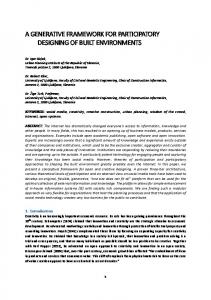
Figure 1. Flow diagram of the 5-step TDN methodology.
should be willing to spend to lower these switching costs at the development stage. The TDN methodology consists of the five steps shown in Figure 1. These steps are described in more detail below, using a generic example of designing a system with three potential instantiations (configurations A, B, and C) and are then implemented in the following section (Section 4) in the context of launch vehicle design and operations.
2.1. Designing an Initial Set of Feasible System Configurations The first step involves creating a family or set of independent or point designs, and an associated high-level cost model for their individual development and operation. Such a family can consist of a core system or product platform with options to expand, or it can include wholly unrelated point designs. Creating appropriate point designs is itself a complex process including initial requirements definitions and trade-studies. Important early stage questions include how best to frame requirements, what metrics should measure system performance, how can one incorporate appropriate levels modularity into the system, and to what level of detail should initial design descend? However, the TDN methodology explicitly recognizes that requirements, demand, and metrics are all subject to change as the systems evolves. Using the initial designs as inputs, it determines the “evolvability” of a set of designs in the face of environmental change. TDN thus shifts the emphasis from point designs to a set of system configurations and identifies specific subsystems and interfaces for redesign. Therefore, for the current purposes, we take point designs as inputs, noting that myriad complex systems from nuclear reactors,
Systems Engineering DOI 10.1002/sys
to road networks, to launch vehicles, and their associated cost models have been created in the past.5 Once a set of conceptual designs has been created, the basic elements of life-cycle cost for each point design i can be estimated (see Table I). Nonrecurring costs include initial development, CDi, and the cost of a switch, Csw. The latter is described in more detail below. CDi is often described as DDT&E (design, development, testing, and evaluation), and includes nonrecurring engineering and facilities costs such as design, analysis, testing of subsystems, system integration, system tests, and construction of any support equipment and facilities [Wertz and Larson, 1999]. Fixed recurring costs CFi, are those incurred at every time period regardless of demand and/or expected changes in the operating environment, including labor, facilities, and overhead. For large, complex systems, labor is usually a major driver for fixed recurring cost. Variable recurring cost CVi, is a function of the demand during a given year or time period. It includes operating costs, production materials, and variable labor costs, among other elements. Models of variable recurring cost often take into account benefits of learning, which reduces the cost per unit as a function of cumulative production levels. Regardless of how these three traditional cost-elements are modeled, they are generally used to estimate life cycle cost CLCi of a given design or system configuration i, as a function of the number of periods T, and the demand in each period, Dj: T
CLCi(D, T) = CDi + CFi × T + ∑ CVi(Dj).
(1)
j=1
Discounting (time value of money) can also be included when estimating lifecycle costs which leads to T
CLCi(D, T, r) = CDi + ∑ j=1
CFi + CVi(Dj) (1 + r) j
.
(2)
In this formulation the initial DDT&E costs, CDi,, are not discounted. A large discount rate r will tend to 5 While inputs to TDN can be taken as given for the current paper, the need to develop better methods to represent the design space such that a good set of initial designs can be created is an important area for further development.
TIME-EXPANDED DECISION NETWORKS
reduce the impact of future expenditures on the lifecycle cost relative to the initial expenditures. For commercial systems that generate revenue, Eq. (2) can also include the revenues (with positive sign) and the costs already discussed (with negative sign) in which case Eq. (2) expresses the net present value (NPV) of the system or project.
2.2. Quantifying Switching Costs and Creating a Static Network 2.2.1. Switching Costs Once an initial set of system configurations has been designed along with an estimate of the three traditional cost-elements (DDT&E, fixed, variable) established for each point design, we must now identify the cost of switching between these system configurations. As noted, switching costs are difficult to quantify because they combine direct production costs as well as indirect organizational and political costs associated with learning and changing established operating procedures. For our current purposes we assume that switching costs comprehend two principal elements: 1. Technical cost associated with altering and producing a new configuration and/or technology 2. A premium for organizational change. The first element includes the cost of designing, building, and testing the new system (∆CD) and the cost of retiring the old system (∆CR). Thus, the technical cost of switching from configuration A to B is the incremental cost of developing B, potentially reusing elements of A, plus the cost of retiring those parts of A that are no longer used when transitioning to B: CSW(A, B) = ∆CD(B, A) + ∆CR(A, B).
(3)
One key assumption is that while A and B will not operate concurrently, there can be commonality between A and B. If A and B share common subsystems or are based on common platforms, CD and CR must be estimated using more detailed analysis of which subsystems are re-used and which must be changed. The premium for organizational change, cO, is optional, but can be a function of the number of people (N) involved in designing and operating the technology:
171
CSW(A, B, N) = cO(N) × [∆CD(B, A) + ∆CR(A, B)]. (4) As a whole, adequately quantifying switching costs is a difficult problem which merits further study. Recent work on formal change propagation analysis [Eckert, Clarkson, and Zanker, 2004] provides guidance in this area. One realistic example of how to quantify switching costs is presented below, in the context of launch system design (Section 4). 2.2.2. The Static Network Once switching costs between system configurations have been estimated, they can be placed in a matrix, with original system configurations (“from”) on the rows and new system configurations (“to”) as the columns. To take a generic example, imagine three possible point designs for a given system: A, B, C. The cost of switching from each to each, CSW(A, B), is placed in a matrix (Table II.). Numbers at each cell in the matrix represent the nondiscounted cost of switching from the ith row (configuration) to the jth column (configuration). It should be clear that these can only represent estimated switching costs, as the actual switching costs may turn out to be different once a switch is actually executed in the future. The matrix is not necessarily symmetric. The entries on the main diagonal are zero, indicating that there is no direct switching cost associated with remaining in the same system configuration. This matrix is formally equivalent to what is called a weighted node-node adjacency matrix in network flow theory and graph theory more generally [Ford and Fulkerson, 1962; Ahuja, Magnanti, and Orlin, 1993]. That is, the matrix of switching costs defines a network whose nodes are the point-designs (configurations) and whose directed arc weights are the switching costs according to Eq. (3) or (4). The resulting graph is represented in Figure 2. We call this representation a “static network.” It covers all possible switches between the three systems at any given point in time. Because all n nodes in the graph are connected to all nodes as well as to themselves, as a rule the number of arcs in this static network will be n2. It is important to note that here the cost of not switching, that is, staying at the same node in the static network, is zero. This is denoted by the fact that
Table II. Generic Switching Cost Matrix for System Configurations A, B, and C
Systems Engineering DOI 10.1002/sys
172
SILVER AND DE WECK
Figure 2. Graph representation of the switching cost matrix between A, B, and C, representing a partial static network.
an arc from a node back to itself is zero. This does not mean that the cost for keeping the system operating in that configuration is zero—there are still fixed and variable recurring costs, as described below. 2.2.3. Completing the Static Network To frame the system’s life-cycle as a dynamic network flow problem we must add costs associated with developing and operating the system in the first place [see Eqs. (1) and (2)]. Then we must add the element of time to each link. The costs associated with operating each system configuration (CD, CF, CV) on the static network above can be coded into the network as follows. Let N represent the static switching network defined above (Fig. 2) consisting of a set of nodes (point designs) P0, P1, P2, ...., Pn and directed arcs associated with switching costs, CSW(X, Y). Let Pij represent the directional arc from node Pi to node Pj. Associate the self-loops (that is, all arcs from a node to itself Pii) with the sum of fixed recurring and variable recurring cost elements for that configuration, i, during one time period ∆T: Pii = CFi + CVi(Dj)
(undiscounted).
(5)
Now create a source node S and a sink node Z and connect them both to all nodes with appropriate directional arcs. Associate all arcs Psi flowing from the source to the point designs with the initial development cost of design i, PDi. This represents the DDT&E cost of the initially chosen configuration. Associate all arcs flowing from point designs i with the sink Piz with the cost = 0.6 The result is a static network (Fig. 3) with all 6 Making all sink arcs = 0 makes the assumption that there are no retirement costs associated with the system at the end of its lifecycle. Retirement costs could be encoded into the network at these arcs as future work.
Systems Engineering DOI 10.1002/sys
Figure 3. Complete static network representing switching and staying costs, as well as development costs. Development is represented by the dotted line from source S to all initial nodes. Retirement is represented by the dotted lines to the sink Z.
information relevant to the life-cycle cost, as a function of demand, encoded in the arcs.
2.3. Creating the Time Expanded Network The goal of the TDN is to capture the cost of operating and switching system configurations through time, seeking least-cost paths through the network as a function of changing operational requirements such as demand. The network above captures all possible development paths during a system’s life-cycle assuming the set of configurations represented in the initial static network, but it is not dynamic—that is, it does not include the element of time. The introduction of time into a directed network transforms it into a dynamic network flow problem. The generic problem involves finding min or max-cost flows from a source S to a sink Z, in a directed network with transversal costs c. Dynamic network flow problems further associate each arc with two variables: traversal cost c and a traversal time t. Often the reformulated objective is to find the maximum flow that can be sent through the network in time T, where costs represent maximum capacity. A solution
TIME-EXPANDED DECISION NETWORKS
to the maximal dynamic network flow problem was first presented by Ford and Fulkerson [1962] and subsequently elaborated upon in a host of different practical applications, e.g., time-varying traffic flow modeling [Köhler, Langkau, and Skutella, 2002]. Dynamic network flow problems can be solved by reformulating the dynamic network into a time-expanded static network, and then solving a traditional max or min cost flow problem on the resulting static network [Ahuja, Magnanti, and Orlin, 1993]. A time expanded network splits the problem into T time periods, with each node in the original network duplicated at every time period. Arcs connect the nodes depending on traversal period, and the new network contains only cost information for each arc. Methods to reformulate static networks into timeexpanded networks are well established [see Ford and Fulkerson, 1962, pp. 146]. We first divide the life-cycle into T time periods and associate each arc with a traversal time t. For simplicity and generality, let us assume here that each arc in the network (switching or staying) takes exactly one time period ∆T to traverse.7 Each node in the static network is duplicated in each time period, and arcs between these nodes are expanded through the new network-based traversal times t. Figure 4 expands the static network created by hypothetical system configurations A, B, C, into a timeexpanded network over 3 time periods, T1, T2, T3. It is assumed for simplicity that the traversal time associated with each arc is exactly one time period, ∆T. Flow starts at the start node S and ends at the end node Z. Figure 4 represents the development alternatives and costs over a life-cycle, given three system configurations A, B, C and our four elements of cost (CD, CF, CV, CSW); however, one critical element is still missing: If a path through the network includes a switching arc, the “operating arc” during that time period will have been avoided. In other words, a min-cost flow through the above network can selectively chose to avoid costs associated with periods of high-demand by switching before them. In reality, an existing system will continue to operate to meet existing demand while a new system configuration is being developed. We therefore introduce a final distinction, taking a cue from decision theory, between chance nodes and 7 Changes to this assumption can easily be made based on specific modeling needs. Sometimes, for example, switching to a new system will take multiple time periods. These kinds of issues can be addressed in different ways by, for example, changing the length of each time period or changing the cost of switching to take account of the fact that it is really spread of multiple time periods (years). For our modeling purposes in Section 4, we assume that 1 time period is 5 calendar years, and that it corresponds to making major development decisions in context of the budget reviews in the U.S. government.
173
Figure 4. Initial Time-expanded Decision Network (TDN) with three configurations and three time periods.
decision nodes, and thereby decoupling operating period’s costs from switching decisions. This is done by splitting each time period with chance nodes (circles) at the beginning, and decision nodes (squares) at the end. Fixed and recurring costs are incorporated into the sub-arcs following the chance nodes at the beginning of each time period (let us call them chance arcs). Switching costs on the other hand are incorporated into the arcs following the decision nodes at the end of each time period (let us call them decision arcs). The chance arcs represent the costs of operating the system at a level of demand, Dj, in time period Tj. The resulting time-expanded network is shown in Figure 5. Initially, coming out of the start node S-19, a system configuration (A, B, or C) must be chosen which causes capital expenditures for DDT&E. If A is chosen, this amounts to CD(A). At the beginning of time period T1, the demand that will have to be satisfied during this period, D1, is revealed at chance node 1. This allows calculation of the operating costs during that time period (both fixed and variable). Towards the end of the time period we encounter decision node 2. We have to decide whether to remain in configuration A (with no switching costs incurred), or whether to switch to configuration B or C, with the respective switching costs being incurred at that time. This process repeats itself until the last time period T3 at which time the system is retired as indicated by transition to the end node, Z-20. The sequence in which the nodes are numbered is important and will be discussed below.
2.4. Create Scenarios and Run Optimization 2.4.1. Operational Scenarios: Modeling Demand It is now possible to introduce operational scenarios over time, by changing the cost of traversing the chance arcs as a function of operational demand and time-vary-
Systems Engineering DOI 10.1002/sys
174
SILVER AND DE WECK
Figure 5. Refined Time-expanded Decision Network. Chance nodes are circles, decision nodes are squares. Nodes are numbered in topological order.
ing requirements on the system by creating various demand scenarios. Demand scenarios can be deterministic, involving known levels of demand at each period, or they may be probabilistic, in which case multiple instances of the TDN have to be solved, one for each uncertain scenario. A simple way to examine the space of demand possibilities is to create a number of discrete demand profiles that are likely to occur over time (i.e., steadily rising demand, constant demand, falling demand, and a limited combination of the three) and applying these to the network. Another way involves modeling using
Geometric Brownian Motion (GBM) and applying multiple combinations of demand scenarios (Fig. 6) [see Haberfellner and de Weck, 2005]. In all cases the demand scenarios are time-discretized, and the information is injected in the appropriate chance nodes. An important point with respect to the TDN methodology is that the four cost elements can be calculated using separate and standard cost models and then used as inputs to the time-expanded network. That is, the total cost of operating in each time period can be computed as a function of the demand scenario and the particular present state (configuration) of the system,
Figure 6. Geometric Brownian Motion (GBM) model of uncertain demand, ∆T = 1 month, D0 = 50,000, µ = 8% p.a., σ = 40% p.a.—three scenarios are shown, based on de Weck, de Neufville, and Chaize [2004].
Systems Engineering DOI 10.1002/sys
TIME-EXPANDED DECISION NETWORKS
and then these costs can be used as the cost of traversing the chance arcs and decision arcs in each time period. 2.4.2. Optimization: Finding the Shortest Paths The ultimate goal of the TDN methodology is to create a simulation of future states of the system to find the set, or sets, of design configurations that minimize life cycle cost (or maximize NPV) under various demand scenarios. By extension, we want to identify exactly where lowering switching costs may maximize adaptability. The set may, or may not include more than one point design, depending on the relevant ratios of the four cost elements (CD, CF, CV, CSW) and the demand at each time period. In other words, this may or may not involve switching from one design to another during the lifecycle. Once the costs of operation are coded into the chance arcs of the time-expanded network, finding least-cost paths involves implementing standard network optimization algorithms. If no loops exist in the network, as in Figure 5, nodes can be ordered topologically—that is, ordered in terms of how far they are from the source. When this is the case, a simple reaching algorithm can be used to find the shortest path. The so-called reaching algorithm [Ahuja, Magnanti, and Orlin, 1993, Lauschke 2006] can solve the shortest path problem (i.e., the problem of finding the graph geodesic between two given nodes) on an m-edge graph in m steps for an acyclic graph. The reaching algorithm is used in this paper. For each operational scenario a different acyclic path through the TDN may be optimal. Even though one may chose to cycle between configurations, the graph will still be acyclic due to time expansion as discussed above. We are interested in identifying those configurations A, B, C, … that are most often chosen as initial configurations and those switches i → j that are selected most often to switch among these configurations during the lifecycle.
2.5. Modifying System Configurations: Iterative Design Once formulated, the time-expanded decision network model is a powerful tool to help formulate and refine initial point designs as well as identify opportunities for commonality and real options [Trigeorgis, 1996] among these configurations. A real option can be framed simply as a feature embedded “in” or “on” an initial design configuration to lower future switching costs. The TDN can be used in many different ways to creatively identify point designs, and interfaces that may lower future operating costs. By combining myriad demand scenarios and network optimization algorithms, designers can selectively tweak elements of
175
point designs, increasing and decreasing commonality, to see exactly how this affects least-cost operating and development paths through the network. As will be illustrated in the example below (Section 4), this information can be used to exploit high-leverage switches that in turn open vast new operating spaces that would never have been exploited had switching options not been considered and incorporated into previous designs. The TDN method can be incorporating into a computer program that enables systems designers to frame the problem of “design for evolvability” more rigorously, to automate aspects of the analysis process, and to identify relationships between designs and the environment that would be very difficult for humans discover. This does not mean, however, that it automates decision-making. The system designer’s knowledge is crucial and is primarily required in creating and selecting interesting feasible system configurations, modeling the four main elements of cost as well as in capturing the uncertain scenarios. A software program based on this method should therefore be considered an iterative design tool which frees system engineers to creatively develop more evolvable (and thus profitable) systems.
3. SCALING THE METHOD An important question here arises: what is the computational cost of conducting such quantitative scenario planning and how does it scale with number of configurations and number of time periods? This section addresses this question. Of the five steps described above (Fig. 1), the first two are conducted manually. That is, configurations and switching costs are inputs to a TDN program. The program then creates the static network at a computational cost, O(C2), where C is the number of configurations. The next three steps involve creating the time-expanded network, applying demand scenarios to the time-expanded network, and finding shortest paths for each scenario. Creating the time expanded network is generally negligible from a computational (processing time) perspective—it involves creating a matrix with appropriate numbering and enough spaces to account for every node N in the network. Given T time periods and C system configurations, the TDN will have the following number of nodes, including the dummy start and end nodes: N = 2 × C × T + 2.
(6)
The factor of 2 comes from having split each node in Fig. 4 into a chance node and a decision node (see Fig. 5). Memory issues can potentially arise when there
Systems Engineering DOI 10.1002/sys
176
SILVER AND DE WECK
are many system configurations (C > 1000) and many time periods (T > 1000). Generally, however, TDN is intended for analyzing a limited number of configurations, C~O(10–100), for a few major time periods or stages, T~O(10–20) from a strategic perspective, and in this regime TDN performs reasonably well. The real computational costs are incurred during the process of iteratively applying scenarios and finding shortest paths. The two steps which contribute to the computational cost here are the computation of chancearc costs (operating costs) as a function of demand scenario, and the running of the shortest path algorithm. Operating costs are calculated as a function of demand, Dj, in each time period and associated with chance-arcs on the time-expanded network (Fig. 5). Given T time periods and C system configurations, this is simply the number of chance arcs, or C × T calculations per scenario. The time expanded network defined above is acyclic, meaning that it contains no cycles. It is therefore possible to implement the reaching algorithm, to find shortest paths efficiently [Ahuja, Magnanti, and Orlin, 1993]. This is significant, since the number of all possible paths through the time expanded network is # paths = CT.
(7)
Thus, the number of paths increases exponentially with the number of time periods if we were to attempt an exhaustive search of all paths. The reaching algorithm, on the other hand, finds a shortest path in O(M) time, where M is the number of arcs in the network. It has been proven that no other algorithm can have better complexity because any other algorithm would have to at least examine every edge, which would itself take M steps [Ahuja, Magnanti, and Orlin, 1993]. In our case, M = (T − 1) × C2 + C × (T + 2),
(8)
where the first term accounts for the switching arcs (decision arcs) assuming that we can switch from any configuration to any other configuration at any time period, and the second term accounts for the chance arcs as well as the initial development and final retirement arcs. Within each scenario, then, total complexity cost is O(Z), where Z = (T − 1) × C2 + C × (T + 2) + C × T
(9)
For consideration of complexity, this reduces to Eq. (10) for each of S scenarios: O(Z) = C2T + CT + C.
Systems Engineering DOI 10.1002/sys
(10)
Therefore, the computational cost of the TDN method, when implemented in conjunction with the reaching algorithm, scales quadratically with the number of configurations C and linearly with the number of time periods T and scenarios S. The complexity of the method is O(SC 2T).
(11)
This appears to represent a significant improvement over traditional multistage decision trees which are known to branch exponentially—similar to Eq. (7)—as a function of the number of decision states and decision stages. A more detailed comparison of the complexity of TDN with traditional decision trees is left for future work.
4. APPLICATION OF TDN TO THE DESIGN OF HEAVY LIFT LAUNCH VEHICLES The TDN method described above has been programmed as a functional software tool8 and applied to the problem of designing an “evolvable” Heavy Lift Launch Vehicle (HLLV) system for NASA’s Vision for Space Exploration (VSE). This vision calls for the return of human explorers to the surface of the Moon by 2020, followed by crewed Mars missions. There is substantial uncertainty surrounding the number and timing of future missions, primarily due to budgetary fluctuations. Like most large, complex systems, launch vehicle architectures and space system architectures generally suffer from architectural lock-in [Shishko, 2001; Silver, 2005b]. To apply the TDN method to this problem, four different initial vehicle configurations were created— one clean sheet design, one based on Evolved Expendable Launch Vehicles (EELVs), and two based on Shuttle-Derived Vehicle (SDV) alternatives—and related cost elements and switching costs were computed. The methodology was run using 10 plausible scenarios for Lunar and Mars exploration campaigns, and total life-cycle costs were calculated. Initial results demonstrated preferred vehicle configurations, and iterative methods quantified the value of lowering switching costs under a uniform scenario probability distribution.
4.1. Step 1: Initial System Configurations The model was implemented using four point designs (Fig. 7) of interest to NASA during the heavy lift launch decision in support of the 2005 Exploration Systems Architecture Study. The four launch vehicle configurations considered are as follows: 8
Using the Matlab V7.1/Simulink technical computing environment.
TIME-EXPANDED DECISION NETWORKS
177
4. P4 = D: Clean Sheet (CS) Heavy Lift Vehicle; Performance: 105 mt to low earth orbit.
Figure 7. Four launch vehicle point designs used in the TDN application. From left to right: Shuttle Derived A (1); Shuttle Derived B (2); EELV derived C (3); Clean Sheet design D (4).
1. P1 = A: Shuttle Derived (SDV-A) Inline Heavy Lift; 3 Space Shuttle Main Engines; 2 four-segment solid rocket boosters; Performance: 80 metric tons to low earth orbit 2. P2 = B: Shuttle Derived (SDV-B) Inline Heavy Lift; 3 Space Shuttle Main Engines; 4 four-segment solid rocket boosters; Performance: 115 metric tons to low earth orbit 3. P3 = C: Evolved Expendable Launch Vehicle (EELV) derived rocket; Delta V core; 2 Zenith boosters; Performance: 62 metric tons to low earth orbit
An N2 diagram showing the components of the launch vehicle models and implementation of the TDN method is shown in Figure 8. The N2 diagram references steps 1–5 shown in Figure 1. After performance and risk were estimated for each configuration, the first step of the TDN process involved estimating initial development costs for all four vehicles as well as fixed and recurring operating costs as a function of demand (“traffic model”). This was initially done by NASA and supplemented by the authors using traditional cost-estimating tools. For more information on this process and the underlying assumptions, see Silver [2005a].
4.2. Step 2: Calculating Switching Costs and Creating the Static Network The next step involved calculating switching costs between the vehicle configurations shown in Figure 7. As noted above, this depends crucially on the amount of commonality between the systems and any real options (reserved interfaces, extra margins, etc.) embedded in them. Systems can share subsystems at different levels. For example, Shuttle-derived vehicles and EELV derived vehicles might be designed to use common largescale subsystems such as launch pads, with minor alterations. At a deeper level in the system decomposition, two shuttle derived vehicles might share almost all first order subsystems—launch pads, manufacturing
Figure 8. N2 diagram of TDN implementation for the launch vehicle design problem.
Systems Engineering DOI 10.1002/sys
178
SILVER AND DE WECK
Figure 9. Estimating switching cost by decomposing subsystems between SDV configurations ($M).
facilities, rocket boosters, main engines—with alterations only to specific second-order subsystems—i.e., the external fuel tank. To calculate switching costs, then, we must break the system into its constituent subsystems to identify commonality at the appropriate level. To take one example of how point designs can involve commonality at a level deeper than the major subsystem level, imagine four shuttle-derived point designs (Fig. 9): a side-mount configuration with 4-segment solid rock boosters (SRBs); a side mount configuration with 5-segment SRBs; an inline vehicle with 4-segment SRBs; and an inline launch vehicle with 5-segment SRBs. Each of these system configuration pairs has commonality in a different way—some share the same solid rocket boosters, others the layout of cargo to external tank. Calculating switching costs between these systems demands examining how their common elements affect subsystem design. Figure 9 demonstrates how this can be done by decomposing major subsystems and examining how they affect subsystem design, in this case the subsystem is the “facilities,” and the components are specific buildings or parts of these buildings. As the highlights demonstrate, different facilities must be altered depending on whether additional SRBs are added, or if the layout of the external tanks is modified (side mounted
Systems Engineering DOI 10.1002/sys
versus vertically stacked). These elements are not mutually exclusive and therefore the switching costs between each system must take into account what is already built and what has yet to be built. In the TDN path optimization, the resulting switching costs between systems 1, 2, 3, and 4 (shown in Fig. 7) are needed. These are presented in Table III (in units of millions of dollars).
4.3. Step 3: Create Time-Expanded Network and Demand Scenarios Once the four cost elements were determined, we created the time expanded decision network (Fig. 10). In this case we had four system configurations and divided the time horizon into four periods. Each time period was assumed to represent 5 years, so the total life-cycle is 20 years. This TDN has CT = 256 possible scenario-independent paths [Eq. (7)] and by plugging C = 4 and T = 4 into Eq. (8), we obtain M = 72 arcs, some of which are shown in Figure 10. Next the demand scenarios were created. As noted, modeling demand is complex and can be carried out in numerous ways depending on the application. For this application, demand for the launch vehicles takes the form of tons of payload needed to be shipped to lowearth orbit (IMLEO) per time period9 and how many launches this would necessitate. NASA is principally
TIME-EXPANDED DECISION NETWORKS
Table III. Switching Costs ($M) between Four Selected Launch Vehicle Configurations
179
scenario. Two vehicle configurations (1 and 3) were used, and no switches were employed. Figure 11 illustrates the two shortest paths, and Figure 12 shows the total life-cycle cost predicted for each scenario. Scenario 6 resulted in the highest total life cycle cost, because it contained the highest number of both Moon and Mars missions.
4.5. Step 5: Iterative Design concerned with returning to the Moon and possibly sending crewed missions to Mars; therefore, we had to translate variations in kind and timing of Lunar and Mars missions to launch-vehicle demand [see Silver 2005a]. Next, we created ten scenarios based on how many Lunar and Mars missions might be launched during each time period and translated this to different numbers of launches for each vehicle and, by extension, different patterns of operations costs along the chance arcs in the time-expanded network (Fig. 10). The 10 future demand scenarios are shown in Table IV. The underlying assumption of these scenarios is that the Moon will serve as a stepping stone to Mars.
4.4. Step 4: Path Optimization Once the demand scenarios we created and the resulting operations costs coded into the network we ran the network optimization (reaching) algorithm under each scenario. The result was ten different shortest paths through the life-cycle, as a function of each demand
The results demonstrate that two vehicles, namely configuration 1 (SDV-A) and 3 (EELV-derived), respectively, were optimal under different operating regimes. This raises the question: Would it be worthwhile to decrease the switching costs between these two vehicles and, if so, how much should we be willing to pay to do this? This question can be easily answered using TDN. Specifically, we can systematically lower the switching costs between two vehicles in order to determine (a) at what switching cost level switching between the configurations would start to occur under each demand scenario and (b) what the savings would be, if any, in terms of total life-cycle cost. We carried out this numerical experiment, systematically lowered the cost of switching from the EELVderived vehicle, configuration 3, to the shuttle-derived SRB vehicle, configuration 1, from $4 billion to $1 billion, in steps of $1 billion. The results are summarized in Figure 13. The results demonstrate that if the switching cost is set to $4 billion, one switch is made in scenario 8 after two time periods—this is a scenario where we encoun-
Figure 10. The time expanded decision network (TDN) for the launch vehicle case. 9 Based on preliminary architectures, we estimated that a lunar mission required approximately 130 metric tons to lunar orbit, while a Mars mission requires on the order of 600 metric tons to be delivered to Low Earth orbit. Uncertainty in these numbers can be introduced by varying both the frequency of demand (number of missions) and the level of demand (mass of each mission). In our model we varied only frequency.
Systems Engineering DOI 10.1002/sys
180
SILVER AND DE WECK
Table IV. Ten Demand Scenarios for Future Launch Vehicle Usage across Four Time Periodsa
a
The total number of lunar missions (requiring 130 metric tons to LEO) is in light gray, the number of Mars missions (requiring 600 metric tons in LEO) is in dark gray.
Figure 11. Two resulting shortest paths through the life-cycle: vehicles 1 and 3 are chosen.
Systems Engineering DOI 10.1002/sys
TIME-EXPANDED DECISION NETWORKS
181
Figure 12. Total life cycle costs ($ billion) for all ten scenarios.
ter few lunar missions initially and many Mars missions later. As the switching cost is lowered further, switches also occur in other scenarios (see Fig. 13).
4.6. Calculating the Benefit What would be the benefit of lowering switching costs in this way? The answer depends on the exact scenario
Figure 13. Switches as a function of switching cost level between $1 billion and $4 billion.
Systems Engineering DOI 10.1002/sys
182
SILVER AND DE WECK
Figure 14. Total life cycle cost (LCC) as a function of switching cost between EELV (3) and SDV vehicle (1). The lighter bars show average LCC across all 10 scenarios; the darker bars show the LCC for scenario 8 specifically.
that ends up occurring in the future. The simulations demonstrated that if scenario 8 occurs, a switch between the vehicles occurs even at a relatively high switching cost. In this case the savings of lowering switching costs between these vehicles would be high. Another way to present this, however, is to determine how much is saved in terms of expected-cost if each scenario is equally likely. We created ten scenarios (Table IV), so each scenario would have a 10% chance of occurring. Figure 14 illustrates the total life-cycle cost as a function of the switching cost between the vehicles, both for scenario 8 in particular and for the case where every scenario is equally likely. SC_Normal is thIe original case (with switching costs shown in Table III), so it should be used as the baseline. The results demonstrate that indeed, savings are greatest if scenario 8
occurs, but that there are also LCC savings on average across all scenarios. Figure 15 makes this even more apparent. It shows the exact amount saved as switching costs are lowered between the two most-used vehicles (3 and 1). If we think all scenarios are equally likely, we can save up to $600 million on average by lowering the switching costs to $1 billion dollars. If we think that scenario 8 will probably occur, we can save as much as $2.8 billion by lowering the switching cost between configurations 3 and 1 to $1 billion. This therefore tells us specifically how much we should be willing to pay to lower the switching costs to those desired numbers. Switching costs can be lowered by embedding provisions in configuration 3 that will make it easier to switch (make changes) to configuration 1 at a later time. There are a number of ways to accomplish this such as standardization, extra margins, inclusion of interfaces for future expansion. This is an appropriate place to apply the principles of changeability enumerated by Fricke and Schulz [2005]. The benefit obtained from lowering switching costs in a way is the maximum price we would be willing to pay on a real option that allows (but doesn’t require) switching from configuration 3 (EELV) to 1 (SDV) at a later date. If it is cheaper to lower the switching costs than not to switch and incur future costs due to operational inefficiency, then the switching costs should be lowered. If this is not the case, then it makes more sense to keep the switching costs where they are in the initial configuration and accept some amount of lock-in. Two final points should be noted. First, we can weight scenarios as we please rather than resorting to averages. Second, lowering the switching cost might change the performance characteristics of the system, and therefore change the life-cycle costs. This should be taken into account during iterative design.
Figure 15. Total LCC savings as a function of switching cost: average for equally weighted 10 scenarios versus savings for scenario 8 alone.
Systems Engineering DOI 10.1002/sys
TIME-EXPANDED DECISION NETWORKS
5. NOTES ON MODEL FORMULATION The generic TDN modeling framework described in this paper can be implemented in different ways based on specific modeling demands, and applied to a variety of systems and industries. This section reviews some modeling issues raised in this paper including areas for future work: • Complete Information: Classic shortest path algorithms assume perfect information about future operating costs. In reality operators do not know what operating scenarios will exist in the future. This “limit to rationality” can be accounted for by revising the shortest path algorithm to limit the number of future time periods considered at each point in time. However, while academically interesting, this may not be practically useful. The goal for the model is to increase system flexibility and enable practitioners to change their behavior, not to model an operating environment per se. Designing systems that evolve optimally demands realism in potential operating scenarios and carefully considered probabilities of occurrence to identify and design optimal switches, not necessarily realism in operator judgment. • Number of Time Periods: We can split the life-cycle into an arbitrary number of time units with each time unit representing an arbitrary amount of real-world time. Note, however, that the number of potential paths increases exponentially with the number of time periods, T. This is mitigated by the fact that the shortest path algorithm scales linearly with the number of time periods. • Time to switch: Switching time can be modeled in ways similar to classic “project cost curve” problems. In these it is generally assumed that a project is an ordered set of jobs. Each job has an associated normal completion time and a crash completion time, and the cost of doing the job (in our case, making the switch) varies linearly between these two times. Project cost curves have a long history [Ford and Fulkerson, 1962: 151]. • Mixed Strategies: We may want to operate more than one kind of a system configuration at the same time. This can be done by sending more than one unit of flow through the network. This is an area for future study. • Decision Rules: There are a number of ways in which TDN can be used to study the effect of a variety of decision rules on lifecycle cost or NPV. Specifically, the path chosen by the reaching algorithm will always be optimal, since it assumes
183
complete information about the future for each scenario. In an unfolding lifecycle scenario decision-makers will have to make the decision whether to stay or switch based on incomplete information. TDN can be used to study the effectiveness of various decision rules by comparing them to the shortest path baseline. • Transition Rules: As discussed above, at each transition point between time periods (stages) one has to decide whether to remain in the current state or transition to one of the (C – 1) other states. This gives rise to the C2 switching arcs between time periods and the CT total paths. One may reduce the number of paths a priori by introducing so-called transition rules, which prohibit certain switches from occurring. This concept was implemented in de Weck, de Neufville, and Chaize [2004], where the staged deployment of satellite constellations was optimized under demand uncertainty. Instead of allowing switches between all 600 configurations, the number of allowable paths was reduced by (i) forming 15 families of 40 configurations each that shared common subsystems and only allowing switches within each family and (ii) by only allowing switches that would grow the system in terms of capacity. • Operational Flexibility: When actual demand Dj is revealed at a chance node at the beginning of time period j, the fixed and variable cost at this time period may not automatically be determined according to Eq. (5). If capacity exceeds demand, one may deliberately choose to shut down part of the system during period j, in order to temporarily reduce fixed costs. When this is possible, we could potentially extend the TDN method to take into account operational flexibility while being in the ith system configuration, not just switching flexibility between configurations i and j. Concurrent consideration of operational and design flexibility is left for future work. • Impact on Design Cost: When lowering the switching costs from $4 billion to $1 billion in Section 4.5, we did not explicitly say how this would be accomplished. Generally, lowering switching costs will require an increase in upfront design cost. This relationship between switching cost and upfront development cost would be a fruitful area of future research. In an extreme case we may decide to design a system that has zero switching costs to reversibly achieve any of the C system configurations under consideration. Such systems are referred to as reconfigurable systems [Siddiqi, de Weck, and Iagnemma, 2006], since
Systems Engineering DOI 10.1002/sys
184
SILVER AND DE WECK
they can switch between configurations at no or very low cost. The ability to be reconfigurable, however, is often associated with significantly increased system complexity (more actuators, sensors, etc.) and upfront effort. Given an explicit relationship between switching costs and upfront development effort, TDN could be used to find the optimal degree of system flexibility that balances upfront expenditures with ease of downstream switching.
6. APPLICATIONS TDN is a generic modeling methodology that can be applied to a host of system-design problems. In the vein of “real options thinking,” we can distinguish between designing for evolvability at the subsystem level or at the system (architectural) level. In the former case, the each design can be considered an instantiation of one system with modified subsystems, and the switching costs will involve the cost of changing those subsystems. By contrast, the example of designing launch vehicles presented above involved more radical configuration changes at the level of the entire system architecture. More specifically, we envision that TDN could be applied to the following kinds of systems: • Complex Electromechanical Products: Systems in this category, from microchips to automobiles, must resolve a host of often conflicting design requirements in catering to one of many potential target markets. Concepts developed to address these issues such as flexible platforming and adaptation to dynamic market segments can be handled more rigorously with the TDN methodology. • Real-Estate and Building Architecture: Traditional building architecture used to define the “program” for a building as driven by its initial use. This is true for residential construction but also for many public buildings (museums, libraries, etc.) and office buildings. Increasingly, however, there is a realization that building use changes over time and that—in order to reduce future remodeling costs—buildings can be deliberately designed to be evolvable over time. An example of this was provided by Kalligeros and de Weck [2004], where BPs new North Sea Exploration Headquarters in Aberdeen, Scotland, was designed in a modular fashion. • Infrastructure Projects and Strategic Planning: Many large-scale infrastructure projects, from electricity grids to water and gas pipelines, in-
Systems Engineering DOI 10.1002/sys
volve networked structures providing services to diverse populations over long life-cycles. These structures exhibit significant lock-in, with serious consequences if the nature and amount of demand cannot be met. TDN can help design responses to critical scenarios and develop networks with better evolved reaction to match demand shifts. • Airline Expansion Decisions: Airlines create networks of transportation which are shaped by, but can also shape, patterns of demand and operation. Decisions about both network structure and vehicle fleet selection are interdependent, and create significant path dependence for airlines [Taylor and de Weck, 2007]. TDN can help create a mix of fleet selection, routing, and maintenance strategy, which allows for appropriate flexibility in the face of changing demand. • Factory Design Under Uncertainty: Companies in multiple industries face the problem of capacity planning under uncertainty. Once built, factories create a specific fixed and variable cost structure in the face of shifting demand, with significant impact on a company’s bottom line. Often, factors in the environment that indicated that a given factory in a given location would be favorable change rapidly, leaving companies with the decision to operate at lower margins or write off the sunken investment. TDN can be used to design both the factories themselves, and select factory locations, in a way that allows for greater flexibility and profitability over the life-cycle. • Strategic Contracting Decisions: Design and acquisition decisions also depend on a host of contracts and legal constraints among developers, acquires, and operators. Whether for system design, or even in purely business matters, contracts are designed to create lock-in using the legal system, in order to change the incentive structures (cost of switching) among contracting parties [Joskow, 1985]. Contracting decisions that affect the evolution of a system, or a business process, can be made more rigorous by explicitly incorporating the costs of switching (even if the latter are purely legal costs). The TDN methodology can thus be applied in the area of pure business strategy and contracting.
7. CONCLUSIONS TDN represents an advance over similar methods to design and analyze system flexibility. First, it is formulated to enable designers to explicitly address the problem of high switching costs, a
TIME-EXPANDED DECISION NETWORKS
principal cause of architectural lock-in, early in the design process in a clear and rigorous manner. Second, by exploiting the inherent structure of the time-expanded graph, TDN overcomes the problem of exponentially branching development options, a serious impediment to the practical implementation of both real options and decision theory-based design methods. Specifically, by expanding the static switching network in time, we can generate an acyclic graph with M~O(C2T) edges, which can be solved by a shortest path reaching algorithm in M-linear time. This is significantly more efficient than enumerating all potential CT paths for all S scenarios. In this way, TDN reformulates life-cycle evaluation as a network optimization problem with clearly defined user inputs. Third, TDN enables quantitative, user-directed scenario planning. Fourth, TDN lends itself easily to implementation as an iterative computational tool, reducing the cognitive load on system designers and allowing them to concentrate on design alternatives, switching options and development scenarios. Finally, the method is generic, being applicable to any systems and sub-systems where architectural lockin and the high-switching costs are a potential problem. Examples of applications that could use TDN would be the design of a factory under uncertain capacity requirements, or fleet acquisition for an airline under uncertain traffic models, among others. TDN developed from the realization that, if properly framed, switching costs between system configurations define a network whose nodes are point-designs and arc-costs are both operating and switching costs. Using concepts from operations research, this “static network” can be expanded into a “time expanded network” in order to model a complete life-cycle. The time expanded network provides a compact representation of all possible development paths for the set of point designs, and thus avoids exponentially branching development options often encountered in traditional decision theory. Used in conjunction with established cost modeling techniques including the estimation of fixed and variable operating costs, the time-expanded network model can be implemented as a software tool and used iteratively to identify optimal switches and design increasingly complex evolvable systems.
REFERENCES R.K. Ahuja, T.L. Magnanti, and J.B Orlin, Network flows: Theory, algorithms, and applications, Prentice Hall, Englewood Cliffs, NJ, February 1993.
185
K. Arrow, Forward to W.B. Arthur, Increasing returns and path dependence in the economy, University of Michigan Press, Ann Arbor, 1994. K. Arrow, Increasing returns: Historiographic issues and path dependence, Eur J Hist Econ Thought 7 (2000), 171–180. B. Arthur, Competing technologies, increasing returns, and lock-in by historical events, Econ J 99 (1989). W.R. Ashby, Design for a brain: The origin of adaptive behavior. Science Paperbacks, London, 1966. C. Baldwin, and K.B. Clark, Design rules, Volume 1: The power of modularity, MIT Press, Cambridge, MA, 2000. C.M. Christensen, The innovator’s dilemma, Harper Collins, New York, 1997. R. Cowan, Nuclear power reactors: A study in technological lock-in, J Econ Hist 50(3) (September 1990), 541–567. P. David, “Path dependence, its critics and the quest for ‘historical economics,’” Evolution and path dependence in economic ideas: Past and present, P. Garrouste and S. Ioannides (Editors), Edward Elgar, Cheltenham, UK, 2000. O. de Weck and E.S. Suh, Flexible product platforms: Framework and case study, Proc IDETC/CIE 2006 ASME 2006 Int Des Eng Tech Conf Comput Inform Eng Conf, September 10–13, 2006, Philadelphia, PA, DETC 200699163. O. de Weck, R. de Neufville, and M. Chaize, Staged deployment of communications satellite constellations in low Earth orbit, J Aerospace Comput Inform Commun 1 (March 2004), 119–136. A. Dixit, Investment and hysteresis, J Econ Perspectives 6(1) (1992), 107–132. G. Dosi (Editor), Technical change and economic theory, London, New York, Printer Publishers, 1988. C. Eckert, P. Clarkson, and W. Zanker, Change and customisation in complex engineering domains, Res Eng Des 15(1) (2004), 1–21. L.R. Ford Jr. and D.R. Fulkerson, Flows in networks, Princeton University Press, Princeton, NJ, 1962. E. Fricke and A.P. Schulz, Design for changeability (DfC): Principles to enable changes in systems throughout their entire lifecycle, Syst Eng 8(4) (2005), 342–359. R. Haberfellner and O.L. de Weck, Agile SYSTEMS ENGINEERING versus engineering AGILE SYSTEMS, INCOSE 2005 Syst Eng Symp, Rochester, NY, July 10–15, 2005. A.C. Hax, D.L. Wilde, and L. Thurow, The Delta Project: Discovering new sources of profitability in a networked economy, Palgrav, New York, 2001. R. Henderson, Of life cycles real and imaginary: The unexpectedly long old age of optical lithography, Research Policy 24 (July 1995) (Issue 4), 631–643. R.M. Henderson and K.B. Clark, Architectural innovation: The reconfiguration of existing systems and the failure of established firms, Admin Sci Quart 35 (1990), 9–30. J.J. Jarvis and H.D. Ratliff, Some equivalent objectives for dynamic network flow problems, Management Sci 28(1) (January 1982), 106–109.
Systems Engineering DOI 10.1002/sys
186
SILVER AND DE WECK
P.L. Joskow, Vertical integration and long term contracts: The case of coal burning electric generating plants, Working Paper, Massachusetts Institute of Technology, Center for Energy Policy Research, 1985, MIT-EL 85-001 WP. K.C. Kalligeros and O.L. de Weck, Flexible design of commercial systems under market uncertainty: Framework and application, AIAA-2004-4646, 10th AIAA/ISSMO Multidisciplinary Anal Optim Conf, Albany, NY, August 30–September 1, 2004. M. Katz, Systems competition and network effects, J Econ Perspectives 8(2) (1984), 93–115. E. Köhler, K. Langkau, and M. Skutella, Time-expanded graphs for flow-dependent transit times, Lecture Notes in Computer Science, Volume 2461, Springer, Heidelberg, 2002. A. Lauschke, Reaching algorithm, from MathWorld—a Wolfram Web Resource, http://mathworld.wolfram.com/ReachingAlgorithm.html, last accessed October 9, 2006. S.J. Liebowitz and S.E. Margolis, Path dependence, lock-in, and history, J Law Econ Org 11(1) (1995) 205–226. R. Nelson and S. Winter, An evolutionary theory of economic change, Harvard University Press, Cambridge, MA, 1982. E.E. Olson, G.H. Eoyang, R. Beckhard, and P. Vaill, Facilitating organization change: Lessons from complexity science, Wiley, San Francisco, CA, 2001. D.J. Puffert, “Path dependence, network form, and technological change,” History matters: Economic growth, technology, and demographic change, T.W. Guinnane, W.A. Sundstrom, and W. Whatley (Editors), Stanford University Press, 2004. L. Sarsfield, The technology puzzle: Quantitative methods for developing advanced aerospace technology, RAND Corp., Santa Monica, CA, 2001.
C. Shapiro, The theory of business strategy, Rand J Econ 20(1) (1989), 125–137. R. Shishko, Lessons learned from the Space Station Program: The role of life cycle cost, Technical Report, Jet Propulsion Laboratory, Pasadena, CA, 2003. A. Siddiqi, O. de Weck, and K. Iagnemma, Reconfigurability in planetary surface vehicles: Modeling approaches and case study, J Br Interplanet Soc (JBIS) 59 (December 2006) 450–460. M. Silver, Heavy lift launch: When is bigger not better? 1st Space Exploration Conf: Continuing the Voyage of Discovery, Orlando, FL, January 30–31, 2005a, AIAA-20052606. M. Silver and O. de Weck, Designing sustainable launch systems: Flexibility, lock-in, and system evolution, 1st Space Syst Des Conf Proc, Georgia Institute of Technology, November 2005. H.A. Simon, The sciences of the artificial (3rd edition), MIT Press. Cambridge, MA, 1996. C. Taylor and O. de Weck, Coupled vehicle design and network flow optimization for air transportation systems, J Aircraft (2007), in press. L. Trigeorgis (Editor), Real options in capital investment: Models, strategies, and applications, Praeger, 13, 1995. J.M. Utterback, Innovation in industry and the diffusion of technology, Sci NS 183 (February 15, 1974), 620–626. J. Wertz and W. Larson, Space mission analysis and design (3rd edition), Microcosm Press, El Segundo, CA and Springer, London, 1999, p. 786. U. Witt, Lock-in vs. industrial mass Industrial change under network externalities, Int J Indust Org 15 (1997), 753– 773.
Matthew R. Silver is a doctoral student in the Engineering Systems Division at the Massachusetts Institute of Technology. He has a background in basic physical research, systems analysis and design, and management and is currently affiliated with the Strategic Engineering group at the Massachusetts Institute of Technology. Mr. Silver has been a research scientist at the MIT Space Systems Lab for 3 years, where he focused on the analysis and design of complex system architectures, and consulted on technology strategy and transfer for companies such as Payload Systems Inc. Prior to this he worked as a systems engineer at the Canadian Space Agency, where he developed and tested advanced concepts for space exploration. Matt has two masters’ degrees in Aerospace Engineering and Technology and Policy from the Massachusetts Institute of Technology and a bachelor’s degree with double major in Astrophysics and Art History from Williams College.
Olivier L. de Weck is currently an Associate Professor with a dual appointment between the Department of Aeronautics and Astronautics and the Engineering Systems Division (ESD) at MIT. His research interests are in Systems Engineering, Multidisciplinary Design Optimization and Space Systems. In 2001 he obtained a Ph.D. in Aerospace Systems from MIT. From 1987 to 1993 he attended the Swiss Federal Institute of Technology (ETH Zurich) in Switzerland, where he earned a Diplom Ingenieur degree (M.S. equivalent) in industrial engineering. From 1993 to 1997 he served as liaison engineer and later as engineering program manager for the Swiss F/A-18 program at McDonnell Douglas (now Boeing) in St. Louis, MO. He served as the General Chair for the 2nd AIAA Multidisciplinary Design Optimization (MDO) Specialist Conference in 2006 and obtained two best paper awards at the 2004 INCOSE Systems Engineering Conference. His research focus is on Strategic Engineering of complex systems.
Systems Engineering DOI 10.1002/sys