Time Implicit Formulation of a Relaxation Approximation of the Euler ...

Time Implicit Formulation of a Relaxation Approximation of the Euler Equations for Real Gases Christophe Chalons

∗

Université Paris 7 & Laboratoire JLL, U.M.R. 7598, Boˆıte courrier 187, 75252 Paris Cedex 05, France

Frédéric Coquel

†

CNRS & Laboratoire JLL, U.M.R. 7598, Boˆıte courrier 187, 75252 Paris Cedex 05, France

Claude Marmignon

‡

Office National d’Etudes et de Recherches Aérospatiales, BP 72, 92322 Chˆ atillon Cédex, France We propose a new time implicit method for approximating the steady state solutions of the Euler equations for real materials in several space dimensions. The severe nonlinearities in the pressure law are bypassed thanks to a suitable approximation procedure with stiff relaxation of the original governing PDE. This approach has been proved fairly successful in a fully time explicit setting. Here, we answer the open question of the time implicit extension of the procedure. A first natural extension of the classical time explicit scheme is shown to fail in producing discrete solutions which converge in time to a steady state. Strong evidences indicate that the stiff relaxation terms are not properly accounted for in this first approach. We then show how to achieve a well-balanced time implicit method which yields approximate solutions at a perfect steady state.

I.

Statement of the problem

The present work treats the numerical approximation of the steady state weak solutions of the Euler equations for real gases :   t > 0, x ∈ D,  ∂t ρ + ∇. ρw = 0, (1) ∂t ρw + ∇. (ρw ⊗ w + p(U) Id ) = 0,   ∂t ρE + ∇. (ρE + p(U))w = 0,

where D is a bounded domain of Rd with d ≥ 1. The pressure law p(U) is a given smooth function of the unknown U = (ρ, ρw, ρE) in the form: p(U) = p(ρ, ρe) with

ρe = ρE −

||ρw||2 , 2ρ

(2)

with the property that the first order system (1) is hyperbolic, namely c2 (U) = c2 (ρ, ρe) =

1 ∂p ∂p (ρ, ρe) + (p + ρe) (ρ, ρe) > 0, ∂ρ ρ ∂ρe

for all state U in the natural phase space: n o ||ρw||2 ΩU = U = (ρ, ρw, ρE) ∈ Rd+2 /ρ > 0, ρw ∈ Rd , ρE − >0 . 2ρ

(3)

(4)

System (1) is given the following condensed form:

∂t U + ∇. F(U) = 0, ∗ Assistant

professor. researcher. ‡ Research scientist. † CNRS

1 of 15 American Institute of Aeronautics and Astronautics

(5)

with clear definition for the vector-valued flux function F(U) = (Fxj (U))1≤j≤d . In the present work, the pressure laws under consideration are motivated by the physics of complex compressible material. The reader is referred to Menikoff and Plorh9 for a discussion and several examples. First, it is well-known that this nonlinear function p(ρ, ρe) is responsible for the most severe part of nonlinearities in the PDE model (1) : in particular it dictates the nonlinearity properties of the fields associated with the acoustic waves. Then, such nonlinearities make difficult and costly the extension to the frame of real gases of celebrated approximate Riemann solvers introduced in the simple polytropic setting. To tackle these nonlinearities and to allow for an efficient numerical procedure, we propose to adopt a relaxation approach: the weak solutions of the system (1) are approximated by the solutions of a larger but simpler PDE model with relaxation source terms. By simpler, it is understood that the underlying nonlinearities are easier to handle. Motivated by the works Bouchut,1 Chalons and Coquel,3 Coquel et al.5 and Siliciu,11 simplicity is achieved when no longer understanding the pressure p(ρ, ρe) as a nonlinear function but as a new unknown we denote by Π, equipped with its own partial differential equation. This new unknown Π is subject to a relaxation procedure which purpose is to restore the original pressure law p in the regime of an infinite relaxation rate. More precisely, the relaxation PDE model developed in5 ,1 ,3 ,11 reads:   ∂ ρλ + ∇. (ρw)λ = 0, t > 0, x ∈ D,   t  λ ∂t (ρw) + ∇. (ρw ⊗ w + Π Id )λ = 0, (6)  ∂t (ρE)λ + ∇. ((ρE + Π)w)λ = 0,    ∂t (ρΠ)λ + ∇. ((ρΠ + a2 )w)λ = λρλ (p(ρλ , (ρe)λ ) − Πλ ), where the parameter λ > 0 stands for the relaxation coefficient rate. Here, the parameter a is a given real number so that the PDE model (6) is seen to be invariant by rotation. To simplify the notations, the relaxation model (6) is given the following condensed form: ∂t Vλ + ∇. G(Vλ ) = λR(Vλ ),

(7)

with V = (ρ, ρw, ρE, ρΠ), R(V) = (0, 0Rd , 0, ρ(p(ρ, ρe) − Π)) and clear definitions for the vector-valued function G(V) = (Gxj (V))1≤j≤d . The precise role played by the parameter a is explained just hereafter but first, it is worth to stress the reason why (6) is easier to handle than (1). To that purpose, observe that setting λ = 0 in (6) decouples the total energy equation from the others. In other words, the total energy only enters the algebraic relaxation source term via the definition (2) of the original pressure law. This weak coupling is responsible for the following attractive result (see1 for instance): Lemma 1. Let be given a > 0 in (6). Then the first order system in (6) is hyperbolic over the following phase space n o ||ρw||2 ΩV = V = (ρ, ρw, ρE, ρΠ) ∈ Rd+3 /ρ > 0, ρw ∈ Rd , ρE − > 0, ρΠ ∈ R . 2ρ

(8)

Namely, for any given unit vector n = (ni )1≤i≤d ∈ Rd , the matrix A(V, n) =

d X

ni ∇V Gni (V)

i=1

is R-diagonalizable for all V ∈ ΩV , with the following increasingly ordered eigenvalues: λ1 (V, n) = w.n −

a a < λ2 (V, n) = w.n < λ3 (V, n) = w.n + , ρ ρ

(9)

where the intermediate eigenvalue λ2 (V, n) has d + 1 order of multiplicity. In addition, all the fields are linearly degenerate: all the propagating waves behave as linear waves. Observe from the definition (9) that the free real parameter a entering (6) has the dimension of ρc(ρ, ρe), i.e. the dimension of a lagrangian sound speed. In any given direction n ∈ Rd , the extreme waves associated with the eigenvalues λ1 (V, n) and λ3 (V, n) may be thus understood as an approximation of the waves in the original equations (1). But the reported linear degeneracy is in clear contrast with the strong nonlinearities


involved in the original PDE model and stays at the basis of the efficient numerical method to be discussed in the next sections. We now come to highlight the importance of a correct definition of the real parameter a in the procedure of approximation of the solutions of (1) by those of (6). To that purpose, let us rewrite the last governing equation in (6) as follows: (ρΠ)λ = (ρp(ρ, ρe))λ −

1 {∂t (ρΠ)λ + ∇. ((ρΠ + a2 )w)λ }. λ

(10)

So that in the limit of an infinite relaxation rate λ → +∞, Πλ formally coincides with the original pressure law p(ρ, ρe): lim Πλ = p(ρ, ρe). (11) λ→+∞

8

After the pioneering works by Liu and Chen, Levermore and Liu,4 it is known that to prevent a general relaxation procedure from instabilities in the regime of a large parameter λ >> 1, the so-called subcharacteristic conditions, or Whitham conditions, must be met: the eigenvalues (9) of the relaxation PDE model and those of the original system must be properly interlaced. In the present relaxation setting (6) for approximating the solutions of (1), these stability conditions are satisfied provided that the free coefficient a > 0 in (9) upperbounds the exact lagrangian sound speed ρc(ρ, ρe); namely, a > ρ c(U) = ρc(ρ, ρe)

(12)

must be valid for all the states U under consideration. The reader is referred to the quoted works1 ,3 ,5 for a detailed discussion of (12) and its relationship with the validity of entropy inequalities for the relaxation PDE model (6) that are closely related to those of the original equations. In this work, it is worth to briefly shade light on the Whitham condition (12) on the simpler ground of a Chapmann-Enskog expansion. According to this approach, the unknown (ρΠ)λ is given the following expansion for large but finite values of λ > 0: (ρΠ)λ = (ρp(ρ, ρe))λ +

1 1 (ρΠ)λ1 + O( 2 ). λ λ

(13)

The first order corrector (ρΠ)λ1 is found when plugging (13) in the PDE (10) to obtain: (ρΠ)λ = (ρp(ρ, ρe))λ −

1 1 {∂t (ρp(ρ, ρe))λ + ∇. ((ρp(ρ, ρe) + a2 )w)λ } + O( 2 ), λ λ

(14)

so that the first order corrector reads: Πλ1

= − ρ1λ {∂t (ρp(ρ, ρe))λ + ∇. ((ρp(ρ, ρe) + a2 )w)λ } = −{∂t (p(ρ, ρe))λ + wλ .∇(p(ρ, ρe))λ } −

a2 ∇. ρλ

(15)

wλ .

To go further, we notice that the first d + 2 equations in (6) reads as follows at the first order in view of the near-equilibrium identity Πλ = (p(ρ, ρe))λ + O( λ1 ):  λ λ  t > 0, x ∈ D,  ∂t ρ + ∇. (ρw) = 0, λ ∂t (ρw) + ∇. (ρw ⊗ w + p(ρ, ρe) Id )λ = O( λ1 ),   ∂t (ρE)λ + ∇. ((ρE + p(ρ, ρe))w)λ = O( λ1 ), so that classical manipulations prove that smooth solutions of (6) obey at the first order in equation for the original pressure law p(ρ, ρe): 1 ∂t p(ρ, ρe)λ + wλ .∇p(ρ, ρe)λ + ρλ c2 (ρ, ρe)λ ∇. wλ = O( ). λ

1 λ

1 λ

and in

(16)

the next

(17)

As a consequence, the first order corrector Πλ1 in (15) writes equivalently: Πλ1 = −

1 2 (a − (ρλ c(U)λ )2 )∇. wλ . ρλ 3 of 15

American Institute of Aeronautics and Astronautics

(18)

Invoking the expansion (13) with the formula (18), the first order asymptotic system governing the solutions of the relaxation system (6) for large values λ >> 1 then reduces to:  ∂t ρλ + ∇. (ρw)λ     ∂ (ρw)λ + ∇. (ρw ⊗ w + p(ρ, ρe) I )λ t d     ∂t (ρE)λ + ∇. ((ρE + p(ρ, ρe))w)λ

= = =

0, − λ1 ∇. (Πλ1 Id ), 1 1 2 2 λ λ λ ∇. ( ρλ (a − (ρc) ) ∇. w Id ),

=

1 λ ∇.

(19)

( ρ1λ (a2 − (ρc)2 )λ wλ ∇. wλ ).

Observe that (19) takes the form of the original Euler equations (1) but in the presence of a viscous perturbation with viscosity like coefficient λρ1λ (a2 − (ρλ c(U)λ )2 ). As it is well-known, this viscosity coefficient must be positive for the solutions of the near-equilibrium system (19) to be stable: this requirement is nothing but the Whitham condition expressed in (12).

II.

The numerical procedure

We show how to take advantage of the relaxation system (6) in the derivation of an efficient time implicit method for the approximation of the solutions to the original Euler equations (1). We first propose a seemingly natural time implicit formulation of the time explicit procedure which is classically performed in a relaxation setting (see7 ,5 for instance). We prove that such a natural extension fails to produce perfectly steady state approximate solutions: residues stop decreasing after a few order of magnitude to then reach a plateau. We then show how to correct this first extension so as to end up with a robust time implicit method that yields converged in time discrete solutions corresponding to a ten order of magnitude decrease for the residues. For the sake of simplicity in the notations, we only address the case of bidimensionnal problems when focusing on cartesian grids with constant space step ∆x > 0 and ∆y > 0, the extension to curvilinear grids being a classical matter. The time variable is discretized using a constant time step ∆t > 0. The approximate solution Uh (x, y, t), h = max(∆x, ∆y), is sought under the form of a piecewise constant function at each time level tn = n∆t, n ≥ 0. An initial data U0 (x, y) being prescribed for (1), we classically define: Z 1 Uh (x, y, 0) = U0i,j = U0 (x, y)dxdy, i, j ∈ Z, (20) ∆x∆y Cij with (x, y) ∈ Cij = ((i − 12 )∆x, (i + 21 )∆x) × ((j − 21 )∆y, (j + 12 )∆y). The boundary conditions considered in the present work are extremely classical in the setting of the Euler equations: namely far field boundary conditions and wall conditions. Their treatment is a classical matter described for instance in Hirsch.6 Besides, MUSCL second order in space enhancement is used in the forthcoming numerical evidences. We again refer the reader to6 for the required material. II.A.

Revisiting the time explicit procedure

In this section, we briefly revisit the usual approach for deriving time explicit scheme in a relaxation framework. Our main purpose is to put forward that this strategy may be actually reinterpreted as a Roe-type method for the relaxation system (7) (but not for the Euler equations (1)). This equivalence with a Roe method stays at the very basis of the time implicit versions to be discussed in the next paragraph. The discrete solution Uh (x, y, tn ) being known at time tn = n∆t, n ≥ 1, this one is evolved to the next time level thanks to a time explicit finite volume scheme: n Uh (x, y, tn+1 ) ≡ Un+1 i,j = Ui,j −

∆t n ∆t n n (F 1 − Fni− 1 ,j ) − (F 1 − F i,j− 21 ), 2 ∆x i+ 2 ,j ∆y i,j+ 2

(x, y) ∈ Cij ,

(21)

where Fni+ 1 ,j and Fni,j+ 1 must be defined at time tn from two numerical flux functions that are respectively 2 2 consistant with the exact flux functions Fx and Fy in the x and y direction. Their required definition follows from the next classical two steps relaxation procedure (see7 for instance). This approach can be understood as a splitting technique for the relaxation system (6) when setting λ to 0 in a first step and then letting the relaxation parameter λ go to infinity in a second step.


First step: Evolution in time (tn → tn+1− ) Starting from the discrete solution Uh (x, y, tn ), we consider a relaxation approximate solution at time tn setting: Vh (x, y, tn ) = (Uh (x, y, tn ), (ρΠ)h (x, y, tn )), (22) where the relaxation pressure is defined at equilibrium (ρΠ)h (x, y, tn ) = ρh p(ρh , (ρe)h )(x, y, tn ).

(23)

We then solve for times t ∈ [0, ∆t[, ∆t small enough, the following Cauchy problem for the frozen relaxation system (7) with λ = 0: ( ∂t V + ∇. G(V) = 0, t > 0, x ∈ D, (24) V(x, y, 0) = Vh (x, y, tn ). Within the finite volume framework, this amounts to update the relaxation approximate solution at time tn+1− setting in each cell Cij : n+1,− n Vi,j = Vi,j −

∆t n ∆t n n n (G 1 − Gi− (G )− 1 − G 1 i,j− 12 ), 2 ,j ∆x i+ 2 ,j ∆y i,j+ 2

(x, y) ∈ Cij ,

(25)

n n where the definitions of Gi+ and Gi,j+ 1 1 will be given hereafter. ,j 2

2

Second step: relaxation (tn+1− → tn+1 ) In each cell Cij , we solve the following EDO problem in the limit λ → ∞:   ∂t ρλ = 0,    ∂t (ρw)λ = 0,  ∂t (ρE)λ = 0,    ∂t (ρΠ)λ = λρλ (p(ρ, ρe)λ − Πλ ),

(26)

with as initial data V(x, y, ∆t− ) the solution of the Cauchy problem (24) at time ∆t. In other words, the approximate relaxation solution Vh (x, y, tn+1 ) is set at equilibrium at time tn+1 in each cell when keeping unchanged ρ, w and E: n+1− n+1− n+1− ρn+1 , (ρw)n+1 , (ρE)n+1 , i,j = ρi,j i,j = (ρw)i,j i,j = (ρE)i,j

(27)

but redefining the relaxation pressure at tn+1 to enforce equilibrium in agreement with (23) : n+1 n+1 (ρΠ)n+1 i,j = (ρp)(ρi,j , (ρe)i,j ).

(28)

The Euler approximate solution Uh (x, y, tn+1 ) is then defined at time tn+1 in each cell Cij using (27) n+1 n+1 n+1 . (29) Un+1 i,j = ρi,j , (ρw)i,j , (ρE)i,j This concludes the method.

n n , Gi,j+ Let us now give a detailed description of the required numerical fluxes Gi+ 1 in (25) in order to 1 2 ,j 2 n n eventually infer the definition of the required fluxes Fi+ 1 ,j and Fi,j+ 1 in (21). We classicaly take advantage 2 2 n of the invariance by rotation of the relaxation PDE model (6) to focus solely on the definitions of Gi+ 1 2 ,j n n n and thus of Fi+ 1 ,j . The fluxes Gi,j+ 1 and Fi,j+ 1 are given symmetric definitions. Here, the numerical flux 2 2 2 n is built from the Godunov approach when solving a Riemann problem for (6) and with λ = 0 function Gi+ 1 ,j 2 in the x direction. Indeed, denoting Gx the exact flux function in (6) and in the x direction and considering for VL and VR in ΩV , W(.; VL , VR ) the self-similar solution of   x (V) = 0,  ∂t V + ∂x G( (30) VL if x < 0,   V(x, 0) = VR if x > 0,

5 of 15


n then we define the required flux Gi+ as follows: 1 ,j 2

n Gi+ 1 ,j 2

n n = Gx (W(0+ ; Vi,j , Vi+1,j ))

≡ ((Gxρ )ni+ 1 ,j , (Gxρu )ni+ 1 ,j , (Gxρv )ni+ 1 ,j , (GxρE )ni+ 1 ,j , (GxρΠ )ni+ 1 ,j ). 2

2

2

2

(31)

2

Here, u (respectively v) denotes the velocity component in the x (respectively y) direction. Let us precise n n that the states VL ≡ Vi,j and VR ≡ Vi+1,j in (31) necessarily read in view of (22), (23): n n Vi,j = Uni,j , ρni,j pni,j , Vi+1,j = Uni+1,j , ρni+1,j pni+1,j . (32) We are now in a position to define the required numerical flux function n ρv n ρE n Fni+ 1 ,j = ((Fρx )ni+ 1 ,j , (Fρu x )i+ 1 ,j , (Fx )i+ 1 ,j , (Fx )i+ 1 ,j ) from the formula (31) and (27): 2

2

2

2

2

(Fρx )ni+ 1 ,j = (Gxρ )ni+ 1 ,j , 2

2

n ρu n (Fρu x )i+ 1 ,j = (Gx )i+ 1 ,j , 2

2

ρv n n (Fρv x )i+ 1 ,j = (Gx )i+ 1 ,j , 2

(33)

2

n ρE n (FρE x )i+ 1 ,j = (Gx )i+ 1 ,j . 2

2

Observe from (32) that the proposed numerical flux function Fni+ 1 ,j is consistent with the exact flux function 2 Fx . Being given two states VL and VR in ΩV , we now define for the sake of completeness the self-similar solution W(.; VL , VR ) of (30) which expanded form reads:  ∂t ρ + ∂x (ρu) = 0,     2  ∂  t (ρu) + ∂x (ρu + Π) = 0, (34) ∂t (ρv) + ∂x (ρuv) = 0,    ∂t (ρE) + ∂x ((ρE + Π)u) = 0,    ∂t (ρΠ) + ∂x ((ρΠ + a2 (VL , VR )u) = 0,

with initial data V0 (x) = VL , x < 0; VR otherwise. In (34), the coefficient a(VL , VR ) is set to: a(VL , VR ) = max( (ρc)(UL ), (ρc)(UR ) ),

(35)

according to the Whitham condition (12). Proposition 1. Let be given two states VL and VR in ΩV . Choose the coefficient a(VL , VR ) as in (35) and possibly larger so as to verify: σ1 (VL , VR ) = uL −

a(VL , VR ) a(VL , VR ) < σ2 (VL , VR ) = u? (VL , VR ) < σ3 (VL , VR ) = uR + , ρL ρR

with u? (VL , VR ) =

1 1 (uR + uL ) − (ΠR − ΠL ). 2 2a(VL , VR )

Then, the self-similar solution W(., VL , VR ) of the Cauchy problem (34) with initial data: ( VL if x < 0, V0 (x) = VR if x > 0,

(36)

(37)

(38)

is made of four constant states VL , V1 (VL , VR ), V2 (VL , VR ), VR separated by contact discontinuities propagating with speed σi (VL , VR ), i = 1, 2, 3:   VL if xt < σ1 (VL , VR ),    V1 (VL , VR ) if σ1 (VL , VR ) < xt < σ2 (VL , VR ), W(x/t; VL , VR ) = (39) x  V (V , V ) if σ (V , V ) < < σ (V , V ), 2 L R 2 L R 3 L R  t   VR if σ3 (VL , VR ) < xt . 6 of 15


The intermediate states V1 (VL , VR ) and V2 (VL , VR ) belong to the phase space ΩV (i.e. ρ1 (VL , VR ) > 0, ρ2 (VL , VR ) > 0) and are recovered from the next formulae with a = a(VL , VR ): Π? = Π1 = Π2 = 21 (ΠL + ΠR ) − a2 (uR − uL ), 1 u? = u1 = u2 = 21 (uL + uR ) − 2a (ΠR − ΠL ), 1 1 1 ? ρ1 = ρL − a (uL − u ), 1 ρ2

=

1 ρR

− a1 (u? − uR ),

(40)

v1 = vL , v2 = vR , E1 = EL − a1 (Π? u? − ΠL uL ), E2 = ER + a1 (Π? u? − ΠR uR ). n is nothing but the Godunov flux for the quasi-1D According to the definition (31), the numerical flux Gi+ 1 2 ,j relaxation system (34). Due to the property that all the fields of this system are linearly degenerate, see n is algebraically equivalent to the one of a Roe-type Lemma 1, it can be proved that the numerical flux Gi+ 1 2 ,j linearization of the system (34). More precisely we successively have:

Proposition 2. For any given pair of states (VL , VR ) ∈ Ω2V , with the notations of Proposition 1, let us define the following five vectors of R5 :   1  u − a/ρ  L  L    r1 (VL , VR ) =  vL ,   ?  EL + ΠL /ρL − au /ρL  ΠL + a2 /ρL       1 0 0  u?   0   0              r2 (VL , VR ) =  1  , r3 (VL , VR ) =  0  , r4 (VL , VR ) =  0  ,        0   1   0  Π?

0

0



   r5 (VL , VR ) =   

1 uR + a/ρR vR ER + ΠR /ρR + au? /ρR ΠR + a2 /ρR



   ,  

where u? and Π? are given in (40). Then, the family ( ri (VL , VR ) )1≤i≤5 spans R5 , i.e. the matrix R(VL , VR ) = r1 (VL , VR ), r2 (VL , VR ), r3 (VL , VR ), r4 (VL , VR ), r5 (VL , VR )

(41)

is invertible.

Proposition 3. For any given pair of states (VL , VR ) ∈ Ω2V , let us consider the well-defined matrix Ax (VL , VR ) ∈ Mat(R5 ) given by: Ax (VL , VR ) = R(VL , VR )D(VL , VR )R−1 (VL , VR ),

(42)

where R(VL , VR ) is the invertible matrix introduced in (41) and D(VL , VR ) the diagonal matrix defined by: D(VL , VR ) = diag(σ1 (VL , VR ), σ2 (VL , VR ), σ2 (VL , VR ), σ2 (VL , VR ), σ3 (VL , VR )). (43) Then, Ax (VL , VR ) is a Roe-type linearization for the quasi-1D relaxation system (34); namely: (i) Ax (V, V) = ∇V Gx (V), (ii) Ax (VL , VR ) (VR − VL ) = Gx (VR ) − Gx (VL ), (iii) Ax (VL , VR ) is R-diagonalizable. 7 of 15 American Institute of Aeronautics and Astronautics

(44)

Equipped with these notations and results, the main statement of this section is: Theorem 1. For any given pair of states (VL , VR ) ∈ Ω2V , the Godunov numerical flux function for the quasi-1D relaxation system (34) is algebraically equivalent to the following Roe numerical flux function: 1 Gx (VL ) + Gx (VR ) − |Ax (VL , VR )|(VR − VL ) , (45) Gx (W(0+ ; VL , VR )) = 2

where Ax (VL , VR ) denotes the Roe linearization (42).

Let us emphasize that the matrix Ax (VL , VR ) ∈ Mat(R5 ) is a Roe-type linearization for the 5 × 5 quasi-1D relaxation system but not for the 4 × 4 quasi-1D original Euler equations. Let us conclude when underlying n that the numerical flux function in the y direction, Gi,j+ 1 , can be also equivalently reexpressed as a Roe 2 method following symmetric steps. II.B.

A first time implicit method

The two step relaxation procedure we have described in a time explicit framework can be given a straightforward time implicit formulation. For the sake of efficiency, this time implicit method is classically linearized thanks to the existence of a Roe linearization for equivalently reexpressing the numerical fluxes. More precisely, the two steps of the previous section now read: First step: evolution in time (tn → tn+1− ) Solve the following linearized time implicit scheme n+1− n Vi,j = Vi,j −

∆t n+1− ∆t n+1− n+1− n+1− )− ), (G 1 − Gi− (G 1 1 − G i,j− 12 2 ,j ∆x i+ 2 ,j ∆y i,j+ 2

(i, j) ∈ Z2 ,

(46)

where thanks to the equivalent form (45) we have classically set: n+1− n Gi+ = Gi+ 1 1 ,j ,j 2

1 2 (∇V 1 2 (∇V

+

2

+

n n n n Gx (Vi,j ) + |Ax (Vi,j , Vi+1,j )|) δ(Vi,j ) n n n n Gx (Vi+1,j ) − |Ax (Vi,j , Vi+1,j )|) δ(Vi+1,j ),

(47)

where the time increments are defined by: n+1− n n − Vi,j . δ(Vi,j ) = Vi,j

(48)

n+1− A symmetrical definition applies to the numerical flux Gi,j+ 1 in the y direction. 2 n Solving (46) then classically amounts to solve a linear system in the unknown δ(Vi,j )i,j∈Z2 with a pentadiagonal 5 × 5 block matrix. The non-zero entries of a line of the corresponding matrix read

(Lnx )i,j , (Lny )i,j , (Dn )i,j , (Rny )i,j , (Rnx )i,j ,

(49)

where the diagonal 5 × 5 matrix writes Dni,j = Id +

n n n n |Ax (Vi,j , Vi+1,j )| + |Ax (Vi−1,j , Vi,j )| n n n n |Ay (Vi,j , Vi,j+1 )| + |Ay (Vi,j−1 , Vi,j )| ,

∆t 2∆x

∆t + 2∆y

while the extradiagonal 5 × 5 matrices are defined by ∆t n n n (Lnx )i,j = − 2∆x ∇V Gx (Vi−1,j ) + |Ax (Vi−1,j , Vi,j )| , ∆t n n n )| , , Vi+1,j ) − |Ax (Vi,j (Rnx )i,j = + 2∆x ∇V Gx (Vi+1,j

with symmetrical definitions for (Lny )i,j and (Rny )i,j .

Second step: Relaxation (tn+1− → tn+1 ) n+1− From the solution Vi,j of the above linear problem (46), we keep unchanged: n+1− n+1− n+1− , , (ρE)n+1 , (ρw)n+1 ρn+1 i,j = (ρE)i,j i,j = (ρw)i,j i,j = ρi,j


(50)

(51)

while we define so as to enforce equilibrium: n+1 n+1 (ρΠ)n+1 i,j = (ρp)(ρi,j , (ρe)i,j ).

In other words, the second step is kept unchanged. This concludes the presentation of the first time implicit formulation of the relaxation approximation procedure. Despites being natural and robust, this first extension is numerically shown hereafter to fail in producing converged in time discrete solutions. The origin of the failure may be understood as follows. The steady state solutions of the Euler equations (1), namely solutions of ∇. F(U) = 0,

x ∈ D,

(52)

are intended to be recovered from the steady state solutions of the relaxation system (6) ∇. G(Vλ ) − λR(Vλ ) = 0,

x ∈ D,

(53)

in the regime of an infinite relaxation rate λ → ∞. Observe that one cannot expect stationary solutions Vλ of (53) to simultaneously satisfy ∇.G(Vλ ) = 0 and λR(Vλ ) = 0 generally speaking in view of the next result: Lemma 2. Let be given V : D → ΩV a smooth function of the space variables such that: ∇. G(V) = 0

and

R(V) = 0,

x ∈ D,

(54)

simultaneously hold. Then , the smooth function V necessarily obeys: (a2 − ρ2 c2 (ρ, ρe)) ∇. w = 0,

x ∈ D,

(55)

where c(ρ, ρe) is the sound speed introduced in (3). Under the mandatory Whitham condition (12), a smooth function V satisfying (54) and therefore (55) necessarily comes with the property of a divergence free velocity field w, i.e. ∇. w = 0. From ∇. ρw = 0 stated in (54), we would then infer w.∇ρ = 0 and thus either ρ necessarily stays constant or the velocity vanishes. Such conditions are far from being general. Therefore, stationary solutions of (53) do not obey (54) in general. In other words, the singular relaxation source term in (53) must come into proper balance with the flux divergence. Here stays the reason of the reported failure in the proposed time marching strategy for capturing steady state solutions of (52) via those of (53). Indeed, the discussed time marching method intends to restore solutions of (53) on the basis of a splitting strategy in between the flux divergence and the relaxation source term: solve first the frozen relaxation system (6) choosing λ = 0 ∂t V + ∇. G(V) = 0, (56) to then restore the relaxation effects when solving ∂t Vλ − λR(Vλ ) = 0,

(57)

in the limit λ → ∞. Formally, time convergence in this splitting strategy to some stationary solutions V would require ∇. G(V) = 0 together with λR(Vλ ) → 0 in the limit λ → ∞, properties which cannot hold for general solutions of (53). In other words, splitting the relaxation source term from the flux divergence cannot result in a well-balanced approximation of the solutions of (53) and therefore of (52). II.C.

Well-balanced time implicit formulation in a relaxation framework

In the light of the previous section, the correct design of a time implicit relaxation procedure requires to handle simultaneously the relaxation source term with the flux divergence during the first evolution step tn → tn+1− . We propose to adopt the following strategy, still made of two steps for reasons we will explain on due time. First step: evolution in time (tn → tn+1− )


Instead of the the frozen version (24) with λ = 0, we have to approximate at time ∆t the solution of the following Cauchy problem ( ∂t Vλ + ∇. G(Vλ ) = λR(Vλ ), (58) Vλ (x, y, 0) = Vh (x, y, tn ), in the regime of an infinite relaxation rate λ → ∞. The initial data Vh (x, y, tn ) is again built at equilibrium from Uh (x, y, tn ) according to (22)-(23). In order to derive the required approximate solution, let us start from the following direct extension of (46) λ, n+1− λ, n Vi,j = Vi,j −

∆t λ, n+1− ∆t λ, n+1− λ, n+1− λ, n+1− λ, n+1− (G 1 (G − Gi− )− − Gi,j− ) + λ∆tR(Vi,j ), 1 1 1 2 ,j 2 ∆x i+ 2 ,j ∆y i,j+ 2

(59)

which we have to deal with in the limit λ → ∞. To cope with this limit, let us rewrite the last discrete equation in (59) for updating the relaxation pressure, as follows λ, n+1− λ, n+1− ρΠ = ρp(ρ, ρe) i,j i,j (60) n o G λ, 1n+1− −G λ, 1n+1− G λ, n+1− −G λ, n+1− λ, n+1− −(ρp(ρ,ρe))n i+ ,j i,j+ 1 i− ,j i,j− 1 i,j 1 (ρΠ)i,j 2 2 2 2 , + + −λ ∆t ∆x ∆y

which is nothing but a time implicit discrete form of (10). Under the Whitham condition (35) for the sake of stability, we formally let λ go to infinity in (60) to consider the implicit formula n+1− n+1− n+1− . ≡ ρp(ρ, ρw, ρE) = ρp(ρ, ρe) ρΠ i,j

i,j

i,j

To lower the computational effort due to the nonlinear pressure law p(U), we propose to Taylor expand this implicit formula so as to consider the following final definition n+1− n n n+1− n ρΠ = ρp(ρ, ρe) + p(U) + ρ ∂p (U) ρ − ρ i,j i,j ∂ρ i,j i,j i,j (61) ∂p n+1− n+1− n n n − (ρE)ni,j . +(ρ∇w p(U))i,j (ρw)i,j − (ρw)i,j + (ρ ∂ρE (U))i,j (ρE)i,j It is then convenient to recast (61) in terms of the time increments introduced in (48) to get the next identity n ∂p ∂p δ ρni,j + (ρ∇w p(U))ni,j δ (ρw)ni,j + (ρ ∂ρE (U) (U))ni,j δ (ρE)ni,j − δ (ρΠ)ni,j = 0, p(U) + (ρ ∂ρ i,j

(62)

n n since by construction ρΠ = ρp(ρ, ρe) in (23).

i,j

i,j

Equipped with this identity, we are in a position to state the linear problem to be solved in the unknown n δVi,j . In that aim, we define the pentadiogonal 5 × 5 block matrix entering this linear problem from the block matrices previously introduced in (49), (50) and (51) (L˜x )ni,j ,

(L˜y )ni,j ,

˜ n , (D) i,j

(R˜x )ni,j ,

(R˜y )ni,j ,

(63)

where each four first lines of the 5 × 5 matrices corresponds respectively to the four first lines of: (Lx )ni,j ,

(Ly )ni,j ,

(D)ni,j ,

(Ry )ni,j ,

(Rx )ni,j ,

(64)

while solely the last line of each of the 5 × 5 matrices (64) governing the time increments δ(ρΠ) have been modified in the new block line (63) to account for the new update formula (62). Since this formula written n in a given cell Cij only involves the time increment δVi,j , the last line of (L˜x )ni,j , (L˜y )ni,j and (R˜x )ni,j , (R˜y )ni,j are necessarily set identically to the zero line (0, 0, 0, 0, 0), ˜ n reads: while necessarily the last line of the diagonal matrix D ij ∂p n p+ ρ , ∂ρ ij

∂p n ρ , ∂ρu ij

∂p n ρ , ∂ρv ij

ρ

∂p n , ∂ρE ij


−1 .

(65)

At last, the corresponding component of the right side is set to zero so as to restore (62) with (65). This completes the description of the first step in the well-balanced time implicit formulation of the relaxation scheme. The need for a second step stems from the linearized version (61) we have introduced at time level tn+1− to n+1− reduce the computational effort involved in the initial guess (ρΠ)n+1− = (ρp(ρ, ρe))i,j . Since equilibrium i,j is not achieved with the linearized form (61), a second step is required to be in position to restart the procedure from time tn+1 . Since this second step just asks for the identity (ρΠ)n+1 = (ρp(ρ, ρe))n+1 i,j i,j , this step exactly coincides with the second step described in Section II.B. This concludes the presentation of the method.

III.

Numerical illustrations

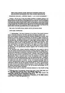
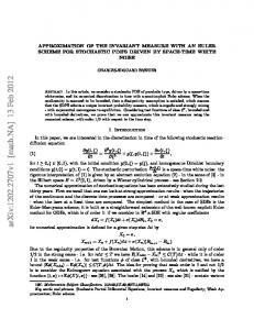
We investigate the performance of the proposed time implicit formulations in the approximation of the steady state solution of the Euler equations over a blunt body. For simplicity, the pressure law is the one of a polytropic gas with adiabatic coefficient γ = 1.2. The freestream conditions follow from a Mach number set to M∞ = 10 and a static pressure p∞ = 40P a and are responsible for a strong bow shock in the steady state solution. The computational domain consists in a curvilinear mesh made of 60 × 48 cells. Figure 1 shows the time history of the L2 norm of the density time derivative obtained using the first time implicit relaxation method. About 15000 time steps have been performed according to the following CFL strategy: the CFL number is set to the constant value 25 during the first 7000 time iterations and decreased down to CFL= 5. Such a strategy makes use of rather small CFL number to prove that the two plateaus achieved in the convergence history is characteristic of a time implicit method which fails to produce converged in time discrete solutions. By contrast, the time history of the L2 -norm of the density time derivative obtained thanks to the well-balanced time implicit relaxation method as depicted in Figure 2 proves perfect convergence in time for the discrete solutions. The results of the two runs are compared, respectively using a constant CFL number set to 25 for the sake of comparison and then choosing an increased value CFL= 200 in order to speed up the calculation. At last, Figure 3 displays the density contours in the steady solution obtained with CFL= 200.

Acknowledgments The second author has been partly financially supported by ONERA during the completion of this work.


Residues

100

10-1

10-2

10-3

10

-4

1

5001

10001 Iteration

Figure 1. Time history of the L2 norm of the density time derivative using the first time implicit scheme


Residues

First implicit method CFL=25 Well-balanced time implicit relaxation method CFL=25

10

-1

10

-3

Well-balanced time implicit relaxation method CFL=200

10-5

10

-7

10-9

1

5001

10001 Iteration

Figure 2. Time history of the L2 norm of the density time derivative using the well-balanced time implicit method


Figure 3. Density contours with the well-balanced time implicit method at CF L = 200


References 1 F. Bouchut, Nonlinear stability of finite volume methods for hyperbolic conservation laws, and well-balanced schemes for source, Frontiers in Mathematics Series, Birkhauser, 2004. 2 C. Chalons, Bilans d’entropie discrets dans l’approximation num´ erique des chocs non classiques. Application aux ´ equations de Navier-Stokes multi-pression et ` a quelques syst` emes visco-capillaires, Th` ese de Doctorat de l’Ecole Polytechnique, in French, 2002. 3 C. Chalons and F. Coquel, Navier-Stokes equations with several independent pressure laws and explicit predictorcorrector schemes, Numer. Math., Vol. 101(3), (2005), pp. 451–478. 4 G.Q. Chen, D. Levermore, and T.P. Liu, Hyperbolic conservation laws with stiff relaxation terms and entropy, Comm. Pure Appl. Math., Vol. 48(7), (1995), pp. 787–830. 5 F. Coquel, E. Godlewski, A. In, B. Perthame, and P. Rascle, Some new Godunov and relaxation methods for two phase flows, Proceedings of the International Conference on Godunov methods : theory and applications, Kluwer Academic, Plenum Publisher, 2001. 6 C. Hirsch, Numerical computation of internal and external flows, John Wiley and Sons, 1990. 7 S. Jin and Z. Xin, The relaxation schemes for systems of conservation laws in arbitrary space dimensions, Comm. Pure Appl. Math., Vol. 48, (1995), pp. 235–276. 8 T.P. Liu, Hyperbolic systems with relaxation, Comm. Math. Phys., Vol. 57, (1987), pp. 153–175. 9 R. Menikoff and B. Plohr, The Riemann problem for fluid flow of real materials, Rev. Mod. Phys., Vol. 61, (1989), pp. 75–130. 10 P.L. Roe, Approximate Riemann solvers, parameter vectors and difference scheme, J. Comp. Phys., Vol. 43, (1981), pp. 357–372. 11 I. Suliciu,On the thermodynamics of fluids with relaxation and phase transitions. I-Fluids with relaxation, Int. J. Eng. Sci., Vol 36, (1998), pp. 921–947.
