Time in State Machines 1. Introduction - Verimag

Fundamenta Informaticae ASM (2005) 1–19

1

IOS Press

Time in State Machines Susanne Graf Verimag, Grenoble, France [email protected]

Andreas Prinz Agder University College, Grimstad, Norway [email protected]

Abstract. State machines are considered a very general means of expressing computations in an implementation-independent way. There are also ways to extend the general state machine framework with distribution aspects. However, there is still no complete agreement when it comes to handling time in this framework. In this article we take a look at existing ways to enhance state machine frameworks. Based on this, we propose a general framework of time extensions for state machines, which we relate to existing approaches. Our mainly addresses time approaches for ASM, because ASM are considered a very general state machine model. Taking this into account, our approach is valid for state-transition systems in general. Keywords: Abstract State Machines, Time, Timed Automata

1.

Introduction

State machines are proven to be a very general means of expressing computations. This is used in the formalism of Abstract State Machines (ASM) [16, 9] that are considered appropriate for giving semantics of a system in terms of its set of possible executions. ASM have been used to define a formal semantics for programming languages (e.g. C [17], C# [7] and Java [26]). It has also been used to define the formal semantics of SDL 2000 [22], the most recent version of SDL [15]. SDL includes an explicit notion of time and time progress, whereas ASM, at least in their initial version, have no explicit means to deal with real-time. Being a very general formalism, it is possible to express any notion of time, and in practise slightly different time models are relevant in different contexts. As time is an important aspect of computations, it is interesting to have an explicit notion of time, and not hiding it in the form ordinary variables. For the definition of the SDL semantics in ASM, we used the ASM time semantics as Address for correspondence: Susanne Graf, Verimag, 2, avenue de Vignate, Grenoble, France, [email protected]

2

S. Graf, A. Prinz / Time in State Machines

proposed in [18] and encountered some problems. The SDL view on time progress is slightly different from the one formalised in [18]. Moreover, ideas to extend the SDL timing to include models with continuous changes lead to a more thorough examination of this issue. This motivated us to summarise some essential properties of timed computations and to derive a methodology for dealing with time in ASM, which we present in this paper. We have studied the main models for timed computations used outside the domain of ASM and we have considered the existing time extensions of ASM. Our aim is to provide a framework for defining timed computations in ASM. For this purpose, we define a set of generic properties of timed computations, which may be used to restrict the set of ”well-formed timed computations”. We tackle the problem by considering the needs for modelling the semantics of concurrent and possibly distributed systems as in the context of model based verification and testing. We want to provide a means to describe executions of timed systems using ASM in a convenient manner. In particular, we do not want to restrict ourselves to the description of time dependent behaviour - as in real-time programming languages - but we want to describe a set of timed computations which means also to express constraints on time progress with respect to system progress. In other words, we do know that some computations take some amount of time and want to specify this. In Section 2, we discuss how to introduce time into the domain of ASM. Moreover, we give some ideas how to express timed properties. Section 3 provides a set of time properties that can be chosen in addition to the basic properties of Section 2. Section 4 discusses the relation of our approach to the existing approaches. In Section 5, we collect the properties we have given to form one possible use case for ASM. The presentation is closed by some conclusions.

2.

An Overview of ASM and Timed Systems

In this section, we discuss general problems occurring when introducing time in a computation model, and then consider the particular case of ASM. Also, our aim is not just to be able to describe a set of timed computations, but to get a means to construct this set of computations (executability). We give an overview of the principles of ASM and discuss some general problems of timed systems.

2.1.

An overview of ASM and their computation model

Abstract State Machines (ASM) [16, 9] were introduced as a general computation model taking concurrency into account explicitly. They are defined starting with a sequential variant and going on to the general distributed case. A sequential ASM algorithm is described by a set of rules applied to states. The notion of state in ASM is very general1 , but for the discussion of time extensions one can consider without loss of generality that a state is defined by the values of a set of variables (also called locations). The notion of ”atomic step” (called a move) is defined by means of a (arbitrarily complex) rule for assigning a new value to some variables depending on the old state values. In order to model inputs and non determinism, a part of the state space might consist of ”monitored variables” which are under the control of ”the environment” and the values of which can only be read by ”the system”. The possible evolutions of the values of monitored variables can be explicitly restricted by constraints. That means, the behaviour of the environment may be described in a declarative way, whereas the system description is provided in a 1

A state is an algebra and a rule describes a transformation between algebras.


3

constructive way: for any state, a means to construct the (set of) next states is given by the set of possible moves. The semantics of the system is given as the set of possible executions, i.e. countable sequences of states representing possible evolutions from the initial state according to the rules and the constraints on monitored variables. In a distributed ASM, there exist several agents (the number of which may evolve over time), which can read and write some part of the global state and have their own update rules. The semantics of distributed ASMs is given by a set of partially ordered runs, where each of these runs consists of a set of moves, partially ordered by a relation denoted < and each move having a finite number of predecessors. Absence of order between moves expresses independence. In addition, it is required that in any run the moves of each agent are strictly ordered and that rule application is confluent (coherence condition)2 . The set of executions is the set of state sequences induced by all possible linearisations of all runs. In ASM, there exists no predefined notion of trigger. Each agent has ”its rule” which can be applied to any state independently of any other agent or the changes of the environment. However, sometimes the application of the rule does not change the state (empty update set). We will consider these rules to be guarded rules, representing partial functions from global states to global states, and consider only runs without such empty moves. Based on this general setup in ASM, we consider a system description to consist of (a) a description of the initial state (defined as the valuation of a vector of variables), and (b) a description of the state change rules. Rules are described per agent. A rule defines a set of moves (MR ⊆ M ). A run is a subset of moves (R ⊆ M ) satisfying the above mentioned constraints, where each move belongs to an agent.

2.2.

Adding Time to State Transition Systems

The first decision we have to take when adding time concerns the kind of models we consider. There is the general distinction between state-based and event-based models. A state-based model is characterised through an explicit notion of state. This means the description of the system takes care of the state. Events are just used to describe moves between states. This way moves (state changes) are secondary level citizens in this kind of systems. On the other hand, event-based models make events the main parts of the description. States are then only a collection of the moves that happened so far or, to put it differently, the possible events that can happen in the future. In practice, this means that event-based formalisms try to avoid speaking about states, and just speak about possible histories and futures, whereas state-based formalisms speak about states and moves. This means that state-based systems describe more detail of the events and also of the result of them, which are the states. This becomes important especially when a notion of ”system equivalence” is defined. For interactive systems, where the notion of time is most important, equivalence is naturally described in terms of languages or trees of “observable” events. In state based formalism, equivalence is expressed in terms of “observable” states, where the notion of “abstract state” is obtained either by simple projection on a subset of elements of the concrete state or a more complex abstraction. As we are mainly interested in ASM, we focus on state-based models. As event-based systems correspond to abstractions, our results can also be applied to this kind of models. Another preliminary consideration concerns domains. We distinguish the two related possibly dense domains T ime – relating to time points on some time scale – and Duration – relating to distances 2

The coherence condition implies that each sequentialisation of the partially ordered run yields the same result, and vice versa.

4


between time points, with appropriate operations between them. Obviously, the second is more general than the first, but it is often interesting to distinguish them because durations have operations and properties which time doesn’t have (notice that axiomatisations of these domains have been given in earlier work, for an example see [11]). In state-based systems, runs are characterised by states and moves, which are alternating. We need therefore to decide where to attach time and/or durations: to states, to moves, or to both. If durations are attached to moves, we are faced with durative moves, otherwise we have instantaneous moves. We adopt the view point that moves are describing a state change, and that we can associate a time point with such a state change. As we are handling distributed computations, it is essential to have a well defined (partial) state at any time. This boils down to excluding durative moves, because then there is clearly no state defined during the time the move is performed3 . Notice that if the state within a durative move is not explicit, there is no way to define something like an interrupt otherwise than by considering explicitly a smaller move granularity and to verify after each micro move if an interrupt arrived. With an explicit state ”in move”, we need only to refine the granularity ”as needed” and imposed by the environment sending an input. We think it is important that a general formalism like ASM can represent ”event driven systems” directly and not only in an approximated fashion through a fine grained time driven system. This motivates the solution to not associate durations with moves, but to consider that moves take place at certain time points. Another argument starts by looking at states first. If time is part of the state, it turns out that this requires for compositionality and for distributed agents a maximal granularity of time steps: when there is no a priori existing discretisation, the possible time steps of an agent need to be dense (even if in every global computation, in every finite time interval, only a finite number of time points are relevant and exist as states). This is done in a very consequent way within the formalism of HASM [25]. However, we think that this is too complex to be useful for practical applications. This motivates the choice in our framework to not make time part of the state. This brings us to a first property of timed computations: time points are attached to moves. In order to achieve this in a sound way, we have to extend our semantic model. We start with the partially ordered runs of the original ASM definition, and attach time to moves by introducing a function when: Property 1. A state change takes place at a point of time defined by a function when: when : M → T ime This states that moves represent time points. It does not formally exclude the existence of “time progress moves” in which only time progresses and it does also not formally exclude that time is part of the state. But in the following we present a framework in which the necessity of time progress move and time in states can be avoided. There is a semantic function associating a time point with moves; the duration of a state can be defined implicitly as the time passing between the occurrence times of its two adjacent events4 . And we have already explained why we believe that this is a preferable solution. The next property concerns the relationship between the time-induced order and the partial order of moves. A natural minimal requirement is given by 3

As analysed by Lamport et. al. in [23], the undefinedness of durative moves has often only local impact. There are several ways to circumvent this. However, all these workarounds boil down to making the intermediate (undefined) state something defined, as proposed by us. The choice is then between an implicit mechanism and an explicit one. We prefer to have an explicit mechanism for the semantic foundations and to leave the choice of implicit mechanisms for the concrete language to be used (e.g. as a shorthand notation). 4 Considering this interval to be open, left-closed, right closed or closed leads to different frameworks.


5

Property 2. In every run, all causally ordered events are also ordered in time, i.e. ∀m1 , m2 ∈ M • m1 < m2 =⇒ when(m1 ) ≤ when(m2 ). More restrictive requirements on the time ordering are discussed in Section 3.

3.

Timed Frameworks defined by a Set of Axioms

So far, we have shown how to extend an ASM system with time semantically, in the form of timed runs and have given a minimal property of the resulting timed computations. Most frameworks for modelling timed systems suggest that a timed computation should have some additional properties. Such constraints are often either directly reflected in syntactic or semantic restrictions of the framework (for example, in VHDL [3] the fact that causally related events must have a time distance of at least some infinitesimal δ) or imposed as verification conditions in the form of assumptions (this is in particular the case for fairness or non Zenoness constraints). These properties represent axioms of particular timing frameworks which in the context of ASM can be added as constraints. In this section, we discuss a number of such constraints, which are required in existing frameworks. For each property, we evaluate if it is executable or not, i.e. if it is possible to extend an executable framework without the axiom into one including it. In the case of distributed ASM, the most important question of executability is about deciding at any point of execution, which agents can be executed next. Without time, this question is easily answered in that any minimal5 move can be taken next. When duration constraints between arbitrary events are allowed, there might exist runs that satisfy all the constraints, but cannot be constructed step by step by looking only at the past; even arbitrary look-ahead or guesses on future choices of the environment might be necessary. We may consider such specifications as bad specifications and study the influence of the axioms on executability.

3.1.

Global and Local Time and additional Ordering Constraints

In most existing frameworks time is global, that is the time domain is totally ordered6 . As a consequence, any two timed events are either temporally ordered or simultaneous, which decreases the power of partially ordered runs. A notion of local time allows to introduce a partially ordered time domain where some time points may be incomparable, that is neither ordered nor simultaneous. This distinction motivates some variants of property 2 defined in Section 2.2. Property 2 states that in a timed run the time order is not smaller than the causal order. In order to define global time, this restriction must be strengthened. Property 2.1. Global Time: all time stamps of a run are totally ordered, i.e. the partial order of the moves is extended to a total preorder for their occurrence times, i.e. ∀m1 , m2 ∈ M • when(m1 ) ≤ when(m2 ) ∨ when(m2 ) ≤ when(m1 ) Independently of the choice of local or global time, some frameworks impose an even stronger constraint on causally ordered events. Property 2.2. Strict time progress along causal chains: whenever two moves are causally ordered, their occurrence times are strictly ordered, i.e. ∀m1 , m2 ∈ M • m1 < m2 =⇒ when(m1 ) < when(m2 ). 5

With respect to the causal order 6 In general, real numbers are chosen representing a dense time domain.

6


This forbids reaction chains in zero time. When distinct agents are used to represent physical distribution, this property may be required, but often distinct agents are used to express purely descriptive parallelism in a compositional manner, and here reaction chains may express synchronisation or just conjunction of constraints. Some frameworks for distributed systems with a strict notion of local time require an even stronger property implying that time distances can only be measured between causally related moves. Property 2.3. Timed order is not stronger than causal order: causally non related events are not comparable in the timed order, i.e. ∀m1 , m2 ∈ M • m1 ≤ m2 ⇐⇒ when(m1 ) ≤ when(m2 ). This requirement is very strong as it forbids even incidental timed ordering of non causally related moves and it is used mainly in the context of test of distributed systems. This axiom can be satisfied by choosing either a partially ordered time domain or to have a total order on runs (interleaving), but in this case this property adds nothing to property 2. All these axioms represent safety properties which can be used to strengthen the constraint on the occurrence time of the immediate successors of each move. Note that some of these properties may be combined to create stronger constraints.

3.2.

Zeno Computations

So far, we did not justify the choice of a dense time domain but just chose it to be dense. Indeed, a dense time domain allows arbitrary action refinement (making more internal steps visible) because between any two moves always an intermediate move at an intermediate time point can be inserted7 . What is the meaning of density in an individual timed computation of countable length? For example, do we want to allow computations where the occurrence times of the events of a computation converge to some finite time point? This is called a Zeno computation, and in most frameworks considered as an invalid computation, as expressed by the following property. Property 3.1. Absence of Zeno computations: In any infinite run, there is no upper bound of the time values attached with moves, i.e. ∀R isInf inite(R) =⇒ ∀t ∈ T ime ∃m ∈ R • when(m) > t. It might also be useful to require the existence of some discrete duration δ such that any two causally dependent moves which are not at the same time, have a time distance of at least delta8 . Property 3.2. Minimal time distance: There is a lower bound of the time differences between nonsimultaneous causally ordered moves, i.e. ∃δ ∈ Duration ∀R ∀m1 , m2 ∈ R • m1 < m2 =⇒ when(m2 ) − when(m1 ) > δ. 7

It is not necessary per se to have a dense domain for allowing refinement, because in any concrete situation there are only a finite number of refinement steps involving only a finite number of moves in each step (see also [6]). However, in general it is not known in advance, where to put the refinement steps. This means it has to be possible to refine any one step at any time, which is exactly the definition of density. ; Notice also that “rescaling” the time domain amounts to assuming density. In order to do refinement, we only need rationals, not reals, as we just require being able to refine, not to include all fixpoints. Fixpoints are related to Zeno behaviours which in fact we forbid. 8 we allow zero time steps, as they may be forbidden by requiring property 2.2; also, multiple state changes at the same time may then be considered as a single state change.


7

Property 3.2 is strictly stronger than property 3.1, as this second property admits computations where the events of some agent are at time points tn , with tn+1 = tn + n1 . This computation is not Zeno, as tn grows over all bounds, but it does not satisfy property 3b. A weaker version consists in not requiring the bound δ to be uniform for all runs. But this stronger version is more interesting, and it is sometimes used as criterion for defining “implementability” in a distributed setting. Notice that property 3.2 does not exclude the existence of ”time races”, that is, concurrent moves which are arbitrarily close, so that there exists no uniform δ to separate any pair of moves by a discrete observation. It might also be useful to require the existence of some discrete duration δ such that by observing the state (at most) every δ time units, no local state change is missed. We formulate here a strong version, stating that state changes take place at discrete time points. Property 3.3. Events at discrete steps: Any two moves occur either at the same instant or the time differences between their occurrence times are a multiple of a given value, ∃δ ∈ Duration ∀R ∀m1 , m2 ∈ R∃k ∈ N • when(m1 ) − when(m2 ) = k ∗ δ. In the context of timed automata, sufficient syntactic conditions on rules have been given guaranteeing the absence of Zeno computations and verification methods exists for checking that all finite prefixes can be extended to non Zeno computations. Concerning executability, property 3.1 is meaningless for finite prefixes, property 3.2 coincides with property 2.2 for finite prefixes, and property 3.3 is easily executed because it is a safety property9 .

3.3.

Maximal Progress and Urgency

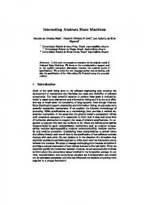
In general, a set of time constraints allows several alternative time stamps to be attached with a move. In this case, the question arises if one should implicitly choose a particular one or make the choice nondeterministically. This brings us to the question if one wants to impose some urgency, for example by requiring maximal progress: Should transitions be taken at the earliest possible time point with respect to all the constraints? endA y = 1 ∧ now ∈ [t + 2, t + 3)

startA

inA

timeout now ≥ t + 3

t := now interrupt x=0

Figure 1.

An example of use of urgency

Example: Let us consider the example in the figure 1 to illustrate the questions related to urgency. The Figure shows some agent Ag and its choices in state inA (meaning that action A has been started). 9

A safety property is a property that can be checked on all finite prefixes of runs, or in the setting of temporal logic, in the form of ”always (some property on the past)”

8


There are 3 possible terminations (a move with three distinct futures), depending on if and when some other agents set the variables x and y; notice that we only represent guards here. An interrupt transition is usually interpreted eager: it is urgent as soon as the environment sets x := 0, let’s say a move mI in an agent AgI , the interrupt or one of the alternatives follows in immediate reaction. A timed run in which the interrupt occurs not ”immediately after” the enabling move, but later, is to be considered invalid10 . For the other two transitions, several interpretations make sense: • An eager interpretation of the endA transition means, it must occur “as soon as its guard holds”, that is, if the environment ha set y := 1, by a move mN of agent AgN , between 2 and 3 time units after the startA transition (which we call for simplicity time 2 or 3). If mN occurs before that interval, endA takes place at time 2, otherwise, it takes place immediately after mN . Notice that, if one of its alternatives is enabled at the time point t at which endA should take place, is enabled as well, the alternative may take place as well until a time point up to t, but not after that. • A delayable interpretation of the endA transition means that under the condition that mN occurs somewhere before 3, it may occur after mN ”at any moment between 2 and 3. But even mN has occurred, let’s say before 2, the interrupt transition may occur at a time ≤ 3 when the condition x = 0 becomes true. Notice that timeout can occur only at a time later than 3, therefore this choice is impossible if mN has occurred at any time up to 3. • Finally the lazy interpretation of the endA transition means that, even if mN occurs before 3, endA may occur up to time 3, but it may also not occur, in which case the timeout transition takes place at some time after 3 (if timeout is lazy) In order to achieve the ”lazy” interpretation of all transitions, no additional axiom is needed. Notice that - even if this is sometimes quite cumbersome - the ”eager” interpretation of all transitions allows achieving the other interpretations by the introduction of explicit moves delaying the concerned move by a duration d as soon as the environment makes true its enabling condition11 . Urgency is expressed simply by the following property: Property 4. Local urgency: The time of each state change of each run is minimal. ∀R • when is minimal Several remarks can be made: • First, urgency makes the time point of the next move deterministic - which is the earliest point of time satisfying its time constraint at which it becomes enabled. Time non-determinism can only be introduced by explicit choices in moves of the form ”choose to wait d”12 and guarantees therefore executability under time constraints. • Second, the choice of the time domain to be reals, makes property 4 incompatible with property 2.213 ; it also makes illegal time constraints for the form ”m takes place at time t > 2”. 10

The interpretation of ”immediately after” depends on the choice of the time progress model. If property 2b is not considered, ”immediately after” means in fact ”at the same point of time”. 11 In the example, endA can be made delayable by splitting it into to several moves “[(if y = 1 then choose d ∈ [now, 3]) followed by (if now = d then endA)] or [if x = 0 then interrupt]” 12 or alternatively ”force another agent to wait d” 13 except if an adequate timing is introduced explicitly to constrain the occurrence time of each reaction


9

Property 4 expresses a local notion of urgency, but we need also to express the fact that from two concurring agents, only the earlier one is allowed. In general properties 4 and 5 are both needed14 . Property 5. Global Urgency: The earliest state change amongst all distributed agents is taken. let minT ime(R, P ) = min(when(m)|m ∈ R \ P ) in ∀R ∀P ∈ pref ix(R) • minT ime(R, P ) = min(minT ime(R0 , P )|R0 ∈ Runs • P ∈ pref ix(R0 ) Notice, that the set Runs above refers to the set of potential runs without taking into account this property. In fact, this property is not exactly of the same kind as the previous ones which qualify runs either as good or bad. Urgency is rather about choosing from a set of potential runs those which are the best runs with respect to some optimality criterion. We could avoid this problem by encoding time as the state of some “time agent” which handles time progress and “encodes” the above constraint into its behaviour, but we definitively want to avoid such a solution. We could also try to not introduce properties 4 and 5, but rather express it explicitly in the specifications by extra moves or conditions in moves. Notice that global urgency is a global constraint on possible time progress — or equivantly on the latest time point at which the next move may take place — which depends on the time constraints of all possible next moves and their urgency15 , but including in each specification such a global constraint is not usable in practise. Concerning executability, urgency is unproblematic as it concerns a decision about the next step, depending only on the actual prefix.

4.

Related Work

In this section, we discuss several frameworks for modelling of timed systems and relate them to the set of properties introduced in the previous section.

4.1.

Timed and Hybrid automata

Timed automata [2] are a model focusing exclusively on timing aspects. A system is represented by a graph16 where each transition represents a state change and is labelled by a constraint on when it can take place. The semantics of a timed automaton is formally defined as a transition system on states defined by a pair consisting of a control state and a time point, where transitions are either discrete moves without time change or time progress moves in the same state. Executions as we have defined them in Section 2 are obtained from a timed automaton execution by the stuttering reduction of the projection to a sequence of discrete states, where the time point at which each discrete move take place is used to define the function when. In timed automata, clocks can be reset to zero in transitions; from then on, at any time they represent the duration since this transition or event until they are reset for the next time. The time model of timed automata is that of global but relative time, where some absolute always increasing value of time may or may not be defined in any particular system. With respect to the set 14

The distinction between local and global urgency is proper to ASM which distinguishes between the case where the three choices in figure 1 are made locally by an agent and the one where they correspond to moves of different agents; in timed automata, local urgency already implies distributed urgency. 15 This constraint corresponds to the time progress condition in timed automata with urgency which exists at semantic level. At syntax level invariants or urgency attributes are used (see section 4.1). 16 or a set of graphs synchronising on the same label

10


of properties of section 3: timed automata impose only the minimal restriction on timed behaviours (property 2), that is, causal chains in zero time are possible. Only non Zeno computations are valid (property 3.1). Timed automata do not require maximal progress (property 4), but have several means to express some notion of urgency. Invariants associated with states can force the system to leave a state on a time condition (like the timeout transition in the example of section 3.3, but without forcing immediate reaction) or by the already mentioned explicit urgency attribute associated with transitions [11, 10], specifying when transitions must be taken. In [9], there is an interesting characterisation of timed automata in terms of ASM. However, this characterisation does still consider time to be external, and does not state which time point would be the next time point - something that is defined within timed automata. Defining an explicit time agent with a rule for timeδ — the already mentioned time progress condition in timed automata — would explain how timed automata work and allow simulation of timed automata in ASM. The time progress condition can be defined for each timed automaton, by an expression that depends in each global control state on the values of all clocks. Hybrid automata [1, 20] are a generalisation of timed automata adding continuous entities other than time. Again, states represent ”modes” in which continuous entities evolve with time according to certain laws - expressed in terms of differential equations - whereas state changes represent discrete changes between different modes - in which the continuous entities may evolve according to different laws. The above mentioned variants of timed automata can also be defined for hybrid automata. In the context of ASM, we can only be interested in projections of the evolutions of continuous quantities to an enumerable set of time points. The axioms of section 3 can be used to define general restrictions on the time points to choose. Urgency is useful to express that all time points of discrete state changes should be included. And in general, system dependent laws are needed as well.

4.2.

Timed Petrinets and Time Extensions in Process Algebras

The aim of time extensions of Process algebras [5] and Petrinets is to express constraints on the occurrence times of synchronisation events. These formalisms have property 1. They are based on global time and impose only the minimal restriction on timed computations as formulated by property 2. Properties of infinite sequences, such as non Zenoness are not part of the framework, but are often added at analysis time as verification conditions or hypotheses. The timed process algebra E-Lotos [21] attaches interval waiting constraints with actions (similar as timed automata). The semantics is defined in a compositional manner: partial actions (which are able to synchronise with other subsystems) are delayable, whereas actions which cannot synchronise with other actions are eager (property 4). A Petrinet (see [27] for an overview) defines a set of partially ordered runs, and time extensions express constraints on the occurrence times of synchronisation events. Petrinet places are waiting states and ”transitions” are actions which may take a variable amount of time. There are several variants of timed Petrinets. We mention here the most interesting one: a transition T takes place when all in-going places have the required amount of tokens and each token has the required “age” defined by a constraint associated with T . Notice that during the possible “waiting phase (tokens are their but not old enough) conflicting transitions may be chosen instead, until including the time point at which T becomes urgent. Depending on the kind of waiting constraints, a transition may become feasible before it becomes urgent or not. That means, synchronisation mechanism is more flexible than the one of timed automata with invariants, but can be expressed using urgency attributes of [11]. Such Petrinets can be represented in


11

ASM, by using either a single agent or some (instantaneous!) agreement on shared variables amongst agents which represent tokens (threads). We would then need immediate reaction and possibly causal chains without time progress of more than length 2.

4.3.

Time Extensions of ASM

In the ASM framework, at syntax level the notion of state is central, whereas in the definition of partially ordered runs, events (moves) play the central role. The time extensions for ASM consider time as a part of the state; this is the only way in which it can be done without extending ASM, but when time is global this leads to many global time progress steps (synchronisations). 4.3.1.

ASM extension allowing only strict time progress

The framework defined in [18] is the one we have used for the definition of the semantics of SDL. In this framework, there is not only a time value associated with each state but also a state with each time value, meaning that consecutive states in a execution must have different times, thus enforcing property 2.2. This poses the problem of immediate reaction for more than two consecutive state changes. 4.3.2.

ASM with actions taking time

In [8], the concepts of [18] have been modified by allowing a state change to take time, meaning that this framework does not use property 1. This model is due to the observation that the application of a set of update rules defining a state change does often not correspond to an event, but to an activity which might have duration. It is not made explicit in [8] what the status of the variables changed during an update is; it may • either keep the old value during the update time (supposing that they remain visible for the environment) • have an undefined value (a read by the environment leads to error) • or have an arbitrary value in the domain (then, it is often better to consider finer granularity of computation) As already mentioned in section 2, such a ”transition”, in the untimed setting considered as a state change, should become in the timed setting a state, the state ”in transition” with some duration. There are two instantaneous state changes associated with an update: ”start transition” - which might render undefined a set of variables, but has otherwise no effect on the state - and ”end transition” - which leads to the updated state. 4.3.3.

Time extensions in AsmL

AsmL [19] is an implementation of ASM for execution and testing of ASM specification. Its real-time concept is based on external time (monitored), where in practice the system time of the computer used for the execution of the model is used as the external source for providing the value of time: it is possible to read time and to react depending on its value. It is also possible to define triggers on time - which in any particular execution may be missed (those actions are lazy and property 4 is not enforced) - and waiting conditions. This enforces properties 2.2 and 3.3. As finite experiments cannot express properties of infinite sequences, properties on infinite sequences (properties 3) are irrelevant.

12


A problem of this approach17 is that time is not abstract but, meaning that the resulting timed execution sequences are only relevant if the execution time for a given set of rules has a well defined relationship to the execution time of the implementation of the model executed at runtime in its target environment18 . Using machine time in is only meaningful for time driven systems under the synchrony assumption, requiring the termination of all internal activities before the next time trigger. Notice that this framework can be usefully adapted to simulated time as proposed here by doing what we want to avoid here, that is (1) introducing the already mentioned time agent letting time progress as required and (2) adding execution time constraints – obtained in separate measurements or by static analysis [28] — directly into the model. This approach is used in several tools for model-based verification with abstract time (see [14, 12, 4]). 4.3.4.

Hybrid ASM

The Hybrid ASM or HASM approach [25] tries to marry the discrete world of state changes with continuous changes of a part of the state. This is done by introducing hyper-real numbers, especially infinitesimal numbers. Using an infinite but hyper-natural number of steps, these infinitesimals add up to ”real” numbers that in turn represent time. This framework imposes a weakened form of property 2.2 which - due to the fact that computations are countable - is covered by the non Zenoness requirement 3.1: an infinite number of steps cannot be done in bounded time. In a simpler form, a similar framework has been chosen in VHDL, where causally related events must be separated by at least some infinitesimal duration, denoted δ, and where only an infinite amount of δ steps have a measurable duration. The main drawback of this framework is that there is no validation method being able to profit from this fine grained time progress concept.

4.4.

SDL

SDL [22] is promoted for the specification and design of distributed real-time systems. Its support for real-time behaviour is essentially limited to timers and the underlying notion of global system time. In SDL, time is considered as external to the system and the system can only react on time progress. Time may pass everywhere, in states, in tasks, in evaluations of guards, and in communications and there is no means to limit these durations (such means are meant to be left to particular implementations). There are two exceptions to this general concept: there exists a notion of ”nodelay” channel where sending and receiving a signal takes place at the same point of time. Also, once a transition has been detected as enabled, it must be taken immediately (property 4). The formal semantics of SDL 2000 has been defined in terms of ASM [15]. In this work we have introduced time as a monitored variable of type real with only very few constraints, in particular the one saying that the values of time must be increasing19 . We had problems to define sending over nodelay channels (which is at the semantic level represented by a sequence of actions) due to the fact that all existing ASM frameworks insist on enforcing property 2.2 (non zero delay between causally related events). 17

which is chosen also in other real-time modelling tools, for example the UML based CASE tool Rhapsody The smaller the observed time intervals are, the more important becomes the probing effect from the model, even if the measured times are relevant for the target platform. Our experiments with Rhapsody confirmed that the results are extremely sensitive to scaling, which is unsurprising, but disappointing from the point of view of the modeller 19 In fact, this is very similar to the approach in [18], mentioned earlier. 18


5.

13

A Proposal for Representing and Handling Time in ASM

In ASM, there exists no predefined notion of time, but an appropriate representation of time may be introduced explicitly, depending on the nature of the system to be modelled. We propose the introduction of some primitive and derived features defining a framework compatible with properties 1 and 2, and where the other properties can be chosen freely.

5.1.

Reading time

In order to be able to constrain the occurrence time of state changes in the rules depending on the occurrence times of earlier event occurrences, we have to make available the occurrence time of events in the states. In ASM, this is done in a similar way as the Self function is defined: we introduce a new function name now into the vocabulary and fix the interpretation of now to be the value of the when function. This allows then to read and store the occurrence time of an event in a variable for later comparison. monitored now : T ime This function is monitored, that is defined by the environment which must respect the chosen set of axioms. The occurrence time of an event may be constrained also by system dependent guards.

5.2.

Local clocks and storing time

In order to obtain an expressive framework, guards must be able to depend on occurrence times of any causally previous event. Timed automata use clocks for making these instants syntactically accessible. In order to introduce a similar mechanism, based on “time stamps”, in ASM, we propose to introduce a domain of M oveN ames similar to P rogramN ames. In addition, we introduce a controlled function time: domain M oveN ames controlled time : M oveN ames → T ime Using this function, the occurrence time of a move can be recorded within the move by a usual assignment time(mN ) := now, where mN is a move name. In the example given later, we implicitly suppose the assignments time(m) := now to be done at every occurrence of a named move m.

5.3.

Urgency and Updates taking time

We have discussed two other concepts that are frequently used in the context of timed systems, moves taking time (representing execution time) and urgency. We have already explained why durative moves are undesirable. they may exist at designer level with a macro replacing a timed move into two instantaneous transitions, and it is easy to imagine macros associating execution times with updates, such that each atomic update is cut into two updates taking place at two different time points. Whenever, the original update is triggered, a possible execution time δ is chosen, and possibly the state modified so as to present to the other agents the intended status “in move”. After time δ the original update takes place. If the agent is reactive or not to the environment in the “in move” state, depends on its “interruptibility”. The information which state changes are taken into account within moves, may be a parameter of the move or globally of the agent We make a similar argument for urgency. We cannot force urgency without the properties 4 and 5, but we can model relaxed urgency in ASM using oracles determinating the time at which a non urgent transition will take place, if no other agent with a conflicting move takes place at an earlier time point.

14


Therefore, we think that this should not be part of the “ASM basics” but one may use macros, either the “urgency attributes” introduced in timed automata with urgency or “urgency predicates” expressing when a transition must be taken immediately if it is enabled.

5.4.

Refinement

An interesting question about a time framework is in how far it supports refinement: • Does it guarantee that adding timing to an untimed specification leads to a refined specification. • Is the framework rich enough to support refinement of time specifications. An elaborate refinement scheme for ASM is presented in [6]. It is a specialisation of the generally accepted notion of refinement, which distinguishes two notions of refinement, based on the comparison of runs. Let SC and SA be to specifications. • SC weakly refines SA when for every run R2 ∈ SC there exists a run R1 ∈ SA such that ref ines(R1 , R2 ) for some notion of refinement between runs stating that R1 can in some sense emulate R2 . • SC strongly refines SA when in addition, for every run in SA there exists a refined run in SC . In our framework, property 2 guarantees that for every reasonable notion of refinement between runs, weak refinement is guaranteed when adding consistent time constraints to an untimed specification. As already stated earlier, (partially) inconsistent time constraints may eliminate untimed runs, and then the strong refinement condition is not satisfied. Some of these specifications may rejected as bad specifications (for example those introducing deadlock), but not all specifications are meant to be refined in the strong way; they may just be abstractions. Especially in time dependent systems, some runs of untimed specifications (using non determinism to simulate time dependent decisions) may be eliminated (e.g. loops defining Zeno runs by property 3.1 or time exceptions handled by some exception handler do never occur due to properties 4 and 5) when timing is introduced. In these cases, it is a question of methodology, if strong or weak refinement is required. The second question concerns support of refinement of already timed specifications. Non Zenoness (property 3.1) is a good requirement for guaranteeing meaningful refinement: it guarantees that any task of finite duration needs to be implemented by a finite number of steps. The properties requiring or allowing reaction in zero-time (urgency, in particular property 5, and not requesting property 2.2) may be considered as suspicious, that is, allowing non implementable specifications. Specifications with zero-time causal chains or urgency are clearly not useful nor desirable for all purposes. Nevertheless, specifications with finite causal chains without time progress • may tremendously simplify reasoning about the correctness of the specification. • do allow consistent refinement as long as steps without time progress are refined steps without time progress. • may be reasonable: for real-time reactive systems controlling a continuous environment, a useful notion of refinement between an abstract specification and its implementation, allows for some approximation for time points of moves and values of controlled values [13, 24]. Also, one might use ASM agents to represent specification level “components” and an implementation of a component system may then consist in eliminating concurrency by merging several specification level components into a single run-time component. In this kind of refinement, several causally related steps in the abstract specification may be refined into just one step in the refined specification.


5.5.

15

Interleaving

An important feature of the definition of distributed abstract state machines is the equivalence between the set partially ordered runs and the set of their sequentialisations. The question is now if by going from runs to timed runs in the way we propose it, and by imposing properties on runs and the set of runs this equivalence might be violated. Indeed, as already stated before, we lose this property with respect to the causal order: only when we are interested exclusively in extending atomic moves with duration without any contrainst when moves may start, time does not have any influence on the causal order. In the context of reactive time-dependent systems adding time, does in general forbid some of the sequentialisations. Property 2 guarantees that timing does not allow to contradict the causal order. We get the same equivalence if we accept that time can refine the causal order and we consider as the relevant partial order the one induced by both the untimed partial order and the time induced order.

6.

Example

In order to illustrate some of the presented ideas, we apply them to the known railroad crossing example in our formalism presented in [18]. The original version gives a controller scanning the environment in a periodic manner where the required periodicity is not specified, it is just supposed that no relevant state change in the environment is missed. Here, we use a more event driven approach and we add trains for being able to specify their arrival rate and time passing in the gate area. agent GATE m1: if opencom then GState:= opening; opencom:=false endif if GState=opening and now-time(m1)= otime then GState:= open endif m2: if closecom then GState:= closing; closecom:=false endif if Gstate=closing and now-time(m2)= ctime then GState:= closed endif agent TRAIN let x = track(Self) m3(x): if Tstate(x)=none then Tstate(x):=one; new(x):=true endif if Tstate(x) = one and now-time(m3(x))≥ ptime then Tstate(x):= none; out(x):= true endif endlet agent CONTROLLER forall x in Tracks m4(x): if new(x) then n:=n+1; new(x):=false endif if CState=ok and ∃x . now-time(m4(x))=wtime then closecom:=true; CState:= nok endif if out(x)=true then n:=n-1 ; endif endforall if n=0 and CState=nok then opencom:= true and Cstate:= ok endif That is, the Gate starts to close when it receives an open command and starts opening when it receives a closed command. It has also states closing and opening representing intermediates states and which are left depending on the time passed since the intermediate state has been entered, represented by conditions of the form now − time(m1) = otime. This allows to receive a new close command in the middle of the opening process – which is realistic – or to state a property saying “there is never a new closing command received in state closing” (as this would make the specification incorrect). The solution in which the move with the effect “gate is closed”

16


takes time, is not satisfactory as it would mean that a close command could either be missed or received only after the end of the current move which could lead to a deadline miss. We added trains, by making the simplifying assumption that on each track there is at most one train in the gate area at any time, recorded in T State. A new train can arrive if the track is empty and it will leave the track at earliest after a delay ptime. The change of a track status is announced to the controller via booleans new(x) and out(x). Finally, the controller uses the booleans new(x) and out(x) to detect incoming and outgoing trains and the interger n to keep track of the number of trains in the gate area. It has also a state remembering the last command sent to the gate. A close command is sent if the gate is opening or open and some delay wtime has passed since a train has been detected, whereas the close command is sent, as soon as the last trains leaves the area (n = 0). This modelling allows the verification of all kind of safety properties which depend on the chosen time constants and the axioms we are going to choose and which in the original model can not be expressed. Notice that we do not model how time progresses, we just suppose that it progresses and we use urgency to assume that no relevant state changes and time points can be missed in any agent. We label certain moves with labels (m1 to m4) and refer to the occurrence time of the last occurrence of a move m by time(m). We may also allow to refer to older occurrences using expressions like time(pre(m)) or since(m) to stand for now − time(m), or using similar constructs. Now we would like to see which are the useful framework properties beyond properties 1 and 2 for this example. We assume here clearly global time (2.1). We clearly don’t want property 2.3 forbidding incidentally identical time points which is useful mainly together with partially ordered time. We may or may not require strict time progress (2.2). But allowing for non strict time progress simplifies reasoning tremendously. Take for example, the case that let’s say trains on track 1 and 2 arrive at the same time in the gate area; this might lead to several possible runs, such as (m3(1) k m3(2)) m4(1, 2) or m3(1) m4(1) m3(2) m4(2). When we allow non strict time progress, the timed continuations after any of them are the same, whereas this is not the case when requiring strict time progress. In refined specification we can still introduce additional agents introducing some nondeterministic delay between the emissions of commands and the moment at which they arrive, replace the tests of the form now − time(m1) = otime by a looser version and possibly suppose that executing commands takes time; this will hopefully still allow us to argue that this new specification is a refinement up to some well defined approximation without divergence with respect to the abstract specification. We clearly want the Gate and the train not to miss any relevant time point and we assume immediate reaction to state changes: if e.g. a “new train” or a “close command” is not recognised and taken into account immediately, we cannot show any reasonable property as the only alternative consists in assuming a possible arbitrary delay. Again, assuming urgency simplifies the model and reasoning about it. For the trains, however, we just want to make sure that a train cannot reach the gate before ptime20 and that a new one can only arrive when the previous one has left. Assuming eagerness would lead to permanently closed gate. All the axioms concerning infinite sequences are not relevant here as there is no possibility to have an infinite amount of steps within finite time. Assuming a regular discrete time scale is not necessary, but could be done. 20

to be exact, some shorter delay ptime’ to be fixed in a similar way as ptime, as ptime states when the train has left the gate


7.

17

Summary and Conclusions

We have have proposed a framework for handling timed specifications with abstract state machines. We have focussed on a framework in which time is attached with state changes, that is moves, whereas time implicitly progresses in states, as in our opinion, it leads to more abstract handling of time related issues. We have given a set of general properties of timed executions and defined their usefulness for different contexts. We have also shown that the main existing frameworks for handling time can be characterised using these axioms. We have proposed some minimal syntax extensions of ASM, allowing to refer to actual time value in a move and to refer to occurrence times of previous moves by means of a time function and special labels associated with moves. We come to the conclusion that important issues, like updates that take time or means for expressing non uniform urgency, should not be directly included in the ASM basics; these are higher level concepts with slightly different needs in different contexts. The fact that in ASM there exists no explicit notion of trigger or input, but only a state, shared between system and environment, complicates the introduction of an appropriate notion of time within this framework. In particular, if time is part of the state, time progress is a state change leading to state changes in all agents. A framework in which time passes in states and transitions represent instants is more flexible than one in which transitions ”take time”, and most formalisms existing in the literature are of this kind. Nevertheless, we do not mean to exclude the possibility to model time by means of just another state variable handled by the environment or more realistically by a set of agents controlling time progress. But this vision of time does not need any extension of ASM and is less well adopted for studying and expressing properties of timed executions. A final observation is that frameworks for modelling timed systems defined independently of ASM do generally admit causal chains taking zero time, at least as long as there are only finitely many zero time steps in a row. All the papers on time extensions of ASM we have studied make an important point out of the requirement of absence of such zero time steps. Maybe this should be reconsidered. We thank the ASM community for many helpful remarks during the period of writing of this article and for many interesting discussions on this topic.

References [1] Alur, R., Courcoubetis, C., Henzinger, T. A., Ho, P.-H.: Hybrid Automata: An Algorithmic Approach to the Specification and Verification of Hybrid Systems, Hybrid Systems 1992, LNCS 736, 1993. [2] Alur, R., Dill, D.: A Theory of Timed Automata, Theoretical Computer Science, 126, 1994, 183–235. [3] Ashenden, P. J.: The VHDL Cookbook. First Edition, Dept. Computer Science University of Adelaide South Australia, 1990. [4] Balarin, F., Lavagno, L., Passerone, C., Watanabe, Y.: Processes, Interfaces and Platforms. Embedded Software Modeling in Metropolis., Embedded Software, Second International Conference, EMSOFT 2002, LNCS 2491, 2002. [5] Bergstra, J. A., Ponse, A., S. A. Smolka, e.: Handbook of Process Algebra, Elsevier, ISBN: 0-444-82830-3, 2001. [6] Börger, E.: The ASM Refinement Method, Formal Asp. of Comput., 15(2-3), 2003, 237–257.

18


[7] Börger, E., Fruja, G., Gervasi, V., Stärk, R.: A high-level modular definition of the semantics of C#, Theoretical Computer Science, 336(2–3), 2005, 235–284. [8] Börger, E., Gurevich, Y., Rosenzweig, D.: The Bakery Algorithm: Yet Another Specification and Verification, in: Specification and Validation Methods (E. Börger, Ed.), Oxford University Press, 1995, 231–243. [9] Börger, E., Stärk, R.: Abstract State Machines - A Method for High-Level System Design and Analysis, Springer Verlag, 2003. [10] Bornot, S., Sifakis, J.: An Algebraic Framework for Urgency, Information and Computation, 163, 2000. [11] Bornot, S., Sifakis, J., Tripakis, S.: Modeling Urgency in Timed Systems, International Symposium: Compositionality - The Significant Difference, LNCS 1536, 1998. [12] Bozga, M., Graf, S., Mounier, L.: IF-2.0: A Validation Environment for Component-Based Real-Time Systems, Proceedings of Conference on Computer Aided Verification, CAV’02, Copenhagen, number 2404 in LNCS, Springer Verlag, June 2002. [13] Caspi, P., Benveniste, A.: Towards an Approximation Theory for Computerised Control, EMSOFT’02 (A. Sangiovanni-Vincentelli, J. Sifakis, Eds.), LNCS 2491, Springer Verlag, Grenoble, October 2002. [14] Closse, E., Poize, M., Pulou, J., Sifakis, J., Venier, P., Weil, D., Yovine, S.: TAXYS: a tool for the developpment and verification real-time embedded systems, Proc. CAV’01, LNCS 2102 (G. Berry, H. Comon, A. Finkel, Eds.), 2001. [15] Group, I.-T. S. G. . S. S.: URL: http://rn.informatik.uni-kl.de/projects/sdl/, 2002. [16] Gurevich, Y.: Evolving Algebras 1993: Lipari Guide, in: Specification and Validation Methods (E. Börger, Ed.), Oxford University Press, 1995, 9–36. [17] Gurevich, Y., Huggins, J.: The Semantics of the C Programming Language, in: Computer Science Logic, CSL’92 (E. Börger, H. Kleine Büning, G. Jäger, S. Martini, M. M. Richter, Eds.), vol. 702 of LNCS, Springer, 1993, 274–309. [18] Gurevich, Y., Huggins, J.: The Railroad Crossing Problem: An Experiment with Instantaneous Actions and Immediate Reactions, Proceedings of CSL’95 (Computer Science Logic), 1092, Springer, 1996. [19] Gurevich, Y., Schulte, W., Campbell, C., Grieskamp, W.: AsmL: The Abstract State Machine Language, Technical report, Version 2.0, Microsoft Research, Redmond, 2002. [20] Henzinger, T. A.: The Theory of Hybrid Automata., Conference on Logic in Computer Science, LICS, 1996. [21] ISO/IEC: E-LOTOS (enhanced LOTOS), 2001. [22] ITU-T: Recommendation Z.100. Specification and Description Language (SDL), Technical Report Z-100, International Telecommunication Union – Standardization Sector, November 2000. [23] Lamport, L.: Time, Clocks and the Ordering of Events in a Distributed System, Communications of the ACM, 21(7), 1978. [24] Mikácˇ , J., Caspi, P.: Temporal refinement in Lustre, Slap’05, Electronic Notes in Theoretical Computer Science, Elsevier, 2005. [25] Rust, H.: Hybrid Abstract State Machines: Using the Hyperreals for Describing Continuous Changes in a Discrete Notation, Abstract State Machines – ASM 2000, International Workshop on Abstract State Machines, Monte Verita, Switzerland, Local Proceedings (Y. Gurevich, P. Kutter, M. Odersky, L. Thiele, Eds.), number 87 in TIK-Report, Swiss Federal Institute of Technology (ETH) Zurich, March 2000. [26] Stärk, R., Schmid, J., Börger, E.: Java and the Java Virtual Machine: Definition, Verification, Validation, Springer-Verlag, 2001.


19

[27] Wang, J.: Timed Petri Nets: Theory and Application, Kluwer, 1998. [28] Yahav, E., Reps, T., Sagiv, M., Wilhelm, R.: Verifying temporal heap properties specified via evolution logic, Proc. European Symp. on Programming, ESOP 2003, LNCS, 2003.