Time localisation of surface defects on optical discs P.F. Odgaard
M.V. Wickerhauser
Department of Control Engineering Frederik Bajersvej 7C Aalborg University DK 9220 Aalborg
[email protected]
Department of Mathematics One Brookings Drive Washington University, St. Louis St. Louis MO 63130
[email protected]
Abstract— Many have experienced problems with their Compact Disc player when a disc with a scratch or a finger print is tried played. One way to improve the playability of discs with such a defect, is to locate the defect in time and then handle it in a special way. As a consequence this time localisation is needed to be as good as possible. Fang’s algorithm for segmentation of the time axis is used since it has good performance in an application like this. Fang’s algorithm has a clear potential for time localisation for some defects and but not for other defects. Instead the normally used threshold is improved to handle eccentricity and localisation of the end of the defect better.
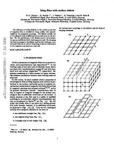
I. I NTRODUCTION Almost everyone has experienced problems with their Compact Disc player (CD player), when they try to play a CD with surface defects. The CD player randomly jumps to another part of the disc or stops playing it. The Optical Pickup Unit (OPU) which is used to retrieve the information from the disc, is kept focused and tracked on the information track by two control loops, since there is no physical contact. The OPU feeds the controllers with indirect measurements of the physical distances in the focus and radial tracking directions, (ef and er ), these distances are illustrated in Fig. 1. During a defect these signals are degenerated, and if not handled in some way the controllers will force the OPU out of focus and radial tracking. Handling these defects requires knowledge of the defects’ time localisations, in other words in which time interval the controller shall react differently to the sensor information. Since the information is used in a feedback control loop, time delays are unwanted. However, the given defect does not vary much from encounter number n to number n+1. This means that time localisation of the defect on encounter n, can be used at the next encounter by adding a reliable prediction of the time to next encounter. The distance between the track is 1.6 µm, this distance is very small compared to the defects. The OPU generates, in addition to ef and er , two residuals which can be used to detect surface defects as scratches, see Fig. 1. Simple threshold method used on the residuals are widely used methods for surface defect detection, see (Philips, 1994), (Andersen et al., 2001) and (Vidal et al., 2001). In (Odgaard et al., 2003b) and (Odgaard et al., 2003a) some more discriminating residuals are described and com-
OPU
er Disc
ef
Track
Fig. 1. The focus error ef is the distance from the focus point of the laser beam to the reflection layer of the disc, the radial error is the distance from the centre of the laser beam to the centre of the track. The OPU emits the laser beam towards the disc surface and computes indirect measurements of ef and er based on the received reflected light. In addition the OPU generates two residuals which can be used to detect surface defects as scratches.
puted. These are computed based on the OPU outputs and models of the OPU and the defects. Time localisation was done based on these signals and a threshold. Defect changes the frequency content of the residuals. This means that the detection problem is similar to the vocal segmentation problem in (Wesfreid and Wickerhauser, 1999), where Fang’s algorithm for segmentation of the time axis was used. Detecting surface defects has some additional problems. Signal noises are different from one disc to another. As a consequence the thresholds need to be adapted to the given noise level. The eccentricity of the disc influences the residuals by changing the received fraction of energy in the OPU. This eccentricity part is mainly the angular velocity of the CD player, which results in a low frequent component in the residuals. Finally, it is important to have a good localisation of the end of the defects, since if it is poor it can result in severe problems for the controllers. It is also important to avoid false positive detections. This paper investigates the potential of the use of Fang’s algorithm for separation of the time axis compared with a simple threshold method. Followed by a description of problems with signal noises and skewness of the disc, these problems are corrected in a way so that false positive detections are avoided.
II. FANG ’ S SEGMENTATION ALGORITHM Fang’s algorithm has been presented by other authors eg. (Wesfreid and Wickerhauser, 1999). This algorithm computes the local maxima of a frequency change function, and the averaged frequency change function which is the average of the instantaneous frequency change function.
0.08
0.06
0.04
A. Instantaneous frequency change function The instantaneous frequency change function computes the change in flatness of the spectrum of the signal. The spectrum is computed with the smooth DCT4 transform, see (Wesfreid and Wickerhauser, 1999). It is the difference between the flatness of the spectrum over [j − l, j + l] with l > 0 and the flatness of the combined spectra over [j − l, j] and [j, j + l]. In this work the flatness of these spectra is measured by the following cost function λ(x0 , x1 , · · · , xn ) = −
n−1 X
|xk |2 log(|xk |2 ).
0.02
0
−0.02
2.658
2.659
2.66
2.661
2.662
2.663
2.664
2.665
2.666
2.667 4
x 10
Fig. 2.
The residual with the first defect. The abscissis is in samples.
(1)
k=0
The DCT4 spectra over [j −l, j +l], [j −l, j] and [j, j +l] are denoted with Aj , Bj and Cj . The instantaneous frequency function (IFC) is in (Wesfreid and Wickerhauser, 1999) defined as IF C(j) = λ(Cj ) − (λ(Aj ) + λ(Bj )),
0.14 0.12 0.1 0.08 0.06
(2)
0.04
where j ∈ {η+l, · · · , N −η−l}, η is the window overlap, and N is the block length. This function oscillates even when the signals are periodic, see (Wesfreid and Wickerhauser, 1999). The IFC is as a consequence low-pass filtered to obtain the averaged frequency change function AFC. This filter is made as follows. If H is a biorthogonal low-pass filter and G its dual, then AF C(j) = Gd H d (IF C(j)),
(3)
0.02 0 −0.02 −0.04
2.47
2.48
2.49
2.5
2.51
2.52
2.53 4
x 10
Fig. 3.
where H d = HHH · · · H, d factors. The segmentation of the time axis is in (Wesfreid and Wickerhauser, 1999) done by finding the local maxima over a given threshold of the AFC signal. These parameters are found by trial and error.
The residual with the second defect. The abscissis is in samples.
0.2
0.15
III. D EFECT DETECTION BASED ON AFC In the following the potential of the AFC method is compared with the normally used threshold. The parameters of the AFC are by trial and error found to be: η = 16, l = 32 and d = 4. The comparison of the algorithms is done by comparing the potentials on three representative residuals with a defect, see Figs. 2-4. The computed AFC of these signals gives the following three Figs. 5-7. By inspection it can be seen that finding the local minima, (due to a sign difference compared with the original algorithm), of the AFC in Fig. 5, gives very good indication of the beginning and end of the defect illustrated in Fig. 2. It is also seen that the AFC in Fig. 6 cannot be used to locate the start and end of
0.1
0.05
0
−0.05 2.592
2.594
2.596
2.598
2.6
2.602
2.604
2.606
2.608 4
x 10
Fig. 4.
The residual with the third defect. The abscissis is in samples.
p. 2
−3
x 10
−2.62
−2.64
−2.66
−2.68
−2.7
−2.72
−2.74
−2.76
−2.78
−2.8 2.658
2.659
2.66
2.661
2.662
2.663
2.664
2.665
2.666
2.667 4
x 10
Fig. 5. The AFC of the residual with the first defect. The abscissis is in samples.
−3
x 10
−2.2
−2.4
−2.6
−2.8
−3
−3.2
−3.4 2.46
2.47
2.48
2.49
2.5
2.51
2.52
2.53
2.54 4
x 10
Fig. 6. The AFC of the residual with the second defect. The abscissis is in samples.
the defect, since its minimum does not locate the beginning and end of the defect. This means that the defects do not change frequency content of the signal in the start and end, but instead during the defect. The AFC of this example looks like a low-pass version of the residual itself, and could be time located by the use of a threshold method. However, some tests indicate that it has to do with chosen parameters in the AFC algorithm, if they are changed such that the AFC of the residual in Fig. 3 has a minimum which is indication in the start and end of the defect. Doing this, the AFC of the first example changes in a way such that minimum cannot be used for detection. The last example, Fig. 4, looks like the first one, Fig. 2, but the AFC of this signal has only one minimum, see Fig. 7, even though this minimum locates the start of the defect, this signal cannot be used to detect the end of it. This means that using the AFC of the residuals in some cases gives a much better time localisation of the defect than by using thresholds since such methods due to the signal noise never can detect the beginning of the defect. The AFC of the first defect seems to do exactly this. Unfortunately it does not have the same good results in the other examples, for Example 2 see Fig. 3. The AFC looks like a low-pass filtered version of the original example, the defect could then be located by using a threshold. However, the DCT used in the AFC is a computation demanding algorithm, in addition to the fact that detection based on the AFC signals needs to be done in a number of ways dependent on the given defect. This means that even though the clear potential of the AFC based detection for some defects represented in Fig. 2 it do shows the same good potentials in situation like in Fig. 3. It cannot be concluded that using Fang’s segmentation method is recommendable in general for time localisation of surface defects on optical discs. IV. C LEANING OF RESIDUALS
−3
x 10
−2.65
−2.7
−2.75
−2.8
−2.85
−2.9
−2.95
−3 2.592
2.594
2.596
2.598
2.6
2.602
2.604
2.606
2.608 4
x 10
Fig. 7. The AFC of the residual with the third defect. The abscissis is in samples.
Another problem with the fault detection is the skewness of the discs. The skewness of the disc results in oscillating references to the focus and radial distances, which are handled by the controllers. The used residuals are designed in a way that they should be decoupled from these distances. However, in addition to these variations the skewness also results in oscillation in the received amount of energy at the detectors. This can be seen as oscillations in the residuals αf [n] and αr [n]. The skewness is illustrated in Fig. 9, where it can be seen that the skew disc does not reflect all the light back to the OPU. A couple of residuals with a clear skewness problem is illustrated by an example from a disc with a scratch and a skewness problem, Fig. 8. If threshold based detection is performed on these residuals the required threshold for detection of the defects is dependent on the defects location on the disc, and if the defect is placed at the top of the oscillation this choice need to be high to ensure no false detections. This means a late detection. p. 3
0.25
0.15
α f αr
α f αr
0.2 0.1 0.15
0.05 r f
α,α
f
α,α
r
0.1
0.05 0
0 −0.05 −0.05
−0.1
0
0.5
1
1.5 samples [n]
2
2.5
−0.1
3
0
0.5
4
x 10
Fig. 8. The two residuals αf [n] and αr [n] computed for a disc with a scratch and a skewness problem.
ef
OPU Fig. 9. Illustration of the skewness of the disc. Notice all the reflected light does not reach the OPU.
The skewness component in the signal is low frequent, almost quasi constant. It can be removed at sample n by subtracting the mean of the block of samples [n−2k −1, n− 1], where k is chosen in a way that the block is not too short or long. Using this method the skewness components are removed from the example, see Fig. 10 V. E XTENDED THRESHOLD To avoid the mean to change during a defect dependent on the defect, these mean blocks need to be much longer than the defect itself. This is not an optimal solution, since a long mean block requires either a large memory or a large number of computations. By inspection it is seen that this skewness component does not change during defects. This means that one way to handle the mean problem is to fix the mean from the sample the defect is detected to the sample one block length after the end of the defect. Noises in αf [n] and αr [n] make it difficult to use an absolute threshold. Instead a relative one to the variance of the non-defect residual parts can be used. To make sure that it is a defect which is detected, the used threshold for the detection of the beginning of the defect needs to be larger than the noises in the residuals. However, having the knowledge of a defect present it is possible to have a lower threshold for detection of the end of the
1
1.5 samples [n]
2
2.5
3 4
x 10
Fig. 10. The skewness component is removed from the two residuals αf [n] and αr [n] computed for a disc with a scratch and a skewness problem.
defect. In other words a multiple threshold is used. Practical experiments indicate that it is a much larger problem if the end is not detected correctly than if the beginning is not. This means that using this multiple threshold, somehow solves two problems. The large threshold for beginning detection, γbeg , limits the numbers of the false positive detections of defects, and the small threshold for end detection, γend , improves the detection of the end of the defect. The mapping from the two residuals to one detection signal, is proposed in (Odgaard et al., 2003a), simply by taking the ∞ norm of the two detections. The detection decision schemes can now be described
(4) d[n] = df [n] dr [n] ∞ , where
AF C(α ˜ f [n]) 1 if var(αf )) > γbeg ∧ df [n − 1] = 0 C(α ˜ f [n]) df [n] = 1 if AFvar(α > γend ∧ df [n − 1] = 1 , f )) 0 if not
(5)
α ˜ f [n] = αf [n] − mean(αf [n − 2k − 1, n − 1]),
(6)
and
AF C(α ˜ r [n]) 1 if var(αr )) > γbeg ∧ dr [n − 1] = 0 C(α ˜ r [n]) dr [n] = 1 if AFvar(α > γend ∧ dr [n − 1] = 1 , r )) 0 if not
(7)
α ˜ r [n] = αr [n] − mean(αr [n − 2k − 1, n − 1]).
(8)
VI. E XPERIMENTAL RESULTS In the following the extended threshold method is compared with a traditional threshold on some test data. A. Experimental setup The experimental setup consists of a CD player, with the three beam single Foucault detector principle, (more detailed descriptions of the CD players are given in (Stan, 1998) and (Bouwhuis et al., 1985)), a PC with an I/O-card, and some p. 4
TABLE I T HE FOUR EXAMPLES OF THE TIME LOCALISATION BASED ON THE TWO THRESHOLD METHODS , AND THE LOCALISATION BY VISUAL
0.25 0.2 0.15 α
f
0.1 0.05
INSPECTION .
0 −0.05 −0.1
0
0.5
1
1.5 samples [n]
2
1.5 samples [n]
2
2.5
3 4
x 10
0.25 0.2 0.15 α
r
0.1 0.05 0 −0.05 −0.1
0
0.5
1
2.5
3 4
ef , er ef er ef er ef er ef er
Inspection 2830-2870 2830-2870 13202-13227 13202-13227 6752-6780 6752-6780 13224-13467 13224-13467
Normal 2843-2865 2837-2863 13204-13223 13205-13222 6754-6776 6757-6773 13445-13465 13446-13464
Extended 2844-2867 2837-2870 13204-13227 13205-13224 6754-6778 6767-6775 13427-13469 13446-13465
x 10
Fig. 11. αf and αr computed of sampled signals with surface defects and eccentricity problems.
hardware in order to connect the CD player with the I/Ocard. Due to the limited computational power of the CPU in the PC, the sample frequency is chosen to 35 kHz. The four detector signals and the two control signals are sampled. By using the built-in controller of the CD player, a number of CDs with certain defects are sampled in a normal operation. Normal operation means that the defects are not severe enough to force the CD player in a state where it cannot play disc, but on the other hand the defect is challenging for the controllers. The experimental work has mainly been focused on real scratches and finger prints, since artificial defects tend to be nice and regular, and they are not really challenging. B. Results The extended and normal threshold methods were applied on some defects. The tested residual signals are illustrated in Fig. 11. Both the simple and the extended threshold methods were used on four different defects in the residuals illustrated in Fig. 11. The thresholds are found such that false positive detections are avoided, meaning that both methods should give almost the same beginning detection but the extended method should give a better end detection. The results are shown in Table VI-B. From the results in Table VI-B it can be seen that the extended threshold method performs better especially in detecting the end of the defects, which are expected due to the multiple thresholds. Detection based on the extended method does not perform much better in detecting the beginning, it performs as well as the normal method, and better in the last example. The chosen example does not show the full potential of the improvement with the removal of the eccentricity, since almost all the defects in this example are at the same area of the disc. This means that the same threshold can be used to detect them all, even though a large eccentricity component is present in the residuals.
VII. C ONCLUSION Fang’s method for segmentation of the time axis, based on the instantaneous frequency change function has potential for time localisation of some kinds of defects, but in other cases, the method does not have the same potential. A threshold method works in all cases even though it for some defects are not as good as the method based on Fang’s algorithm. The threshold method is extended to improve its handling of disc eccentricity and to use a hysteresis threshold, meaning that one is used for detection of the beginning and a smaller one is used for detection of the end. This gives a better time localisation of the end of the surface defect. VIII. ACKNOWLEDGEMENT The authors acknowledge the Danish Technical Research Council, for support to Peter Fogh Odgaard’s Ph.D project, which is a part of a larger research project called WAVES (Wavelets in Audio Visual Electronic Systems), grant no. 56-00-0143. The authors give their thanks to Department of Mathematics, Washington University for hosting the first author during the research for this paper. IX. REFERENCES Andersen, P, T Pedersen, J Stoustrup and E Vidal (2001). Method for improved reading of digital data disc. International patent, no. WO 02/05271 A1. Bouwhuis, W, J Braat, A Huijser, J Pasman, G van Rosmalen and K Schouhamer Immink (1985). Principles of Optical Disc Systems. Adam Hilger Ltd. Odgaard, P.F, J Stoustrup, P Andersen and H.F Mikkelsen (2003a). Estimation of residuals and servo signals for a compact disc player. Submitted for publication. Odgaard, P.F, J Stoustrup, P Andersen and H.F Mikkelsen (2003b). Extracting focus and radial distances, fault features from cd player sensor signals by use of a kalman estimator. Accepted for publication: CDC 2003. Philips (1994). Product specification: Digital servo processor DSIC2, TDA1301T. Philips Semiconductors. Stan, Sorin G. (1998). The CD-ROM drive. Kluwer Academic Publishers. p. 5
Vidal, E, K.G Hansen, R.S Andersen, K.B. Poulsen, J Stoustrup, P Andersen and T.S Pedersen (2001). Linear quadratic control with fault detection in compact disk players. In: Proceedings of the 2001 IEEE International Conference on Control Applications. Mexico City, Mexico.
Wesfreid, Eva and Mladen Victor Wickerhauser (1999). Vocal command signal segmentation and phoneme classification. In: Proceedings of the II Artificial Intelligence Symposium at CIMAF 99 (Alberto A. Ochoa, Ed.). Institute of Cybernetics, Mathematics and Physics (ICIMAF), Habana, Cuba.
p. 6