Time Management Adaptability in Multi-Agent Systems - CiteSeerX

Time Management Adaptability in Multi-Agent Systems Alexander Helleboogh? ?

AgentWise, DistriNet, Department of Computer Science K.U.Leuven, Belgium

[email protected] Tom Holvoet? [email protected]

Danny Weyns? [email protected]

Abstract So far, the main focus of research on adaptability in multi-agent systems (MASs) has been on the agents’ behavior, for example on developing new learning techniques and more flexible action selection mechanisms. However, we introduce a different type of adaptability in MASs, called time management adaptability. Time management adaptability focuses on adaptability in MASs with respect to execution control. First, time management adaptability allows a MAS to be adaptive with respect to its execution platform, anticipating arbitrary and varying timing delays which can violate correctness. Second, time management adaptability allows the execution policy of a MAS to be customized at will to suit the needs of a particular application. In this paper, we discuss the essential aspects of time management adaptability: (1) we introduce time models as a means to explicitly capture the execution policy derived from the application’s execution requirements, (2) we classify and evaluate time management mechanisms which can be used to enforce time models, and (3) we describe a MAS execution control platform which combines both previous aspects to offer high level execution control.

1

Introduction and Motivation

Traditionally, the scope of research on adaptability in multi-agent systems (MASs) has been focused on trying to improve adaptability of individual agents and agent aggregations. As a consequence, the progress made by improving learning techniques and developing more flexible action selection mechanisms and interaction strategies over time is remarkable. This, however, may not prevent us from opening up our perspective and investigating other issues requiring adaptability in MASs. This paper is a first report on ongoing work and introduces time management adaptability as an important source of adaptability with respect to the execution control of MAS applications.

1.1

The Packet-World

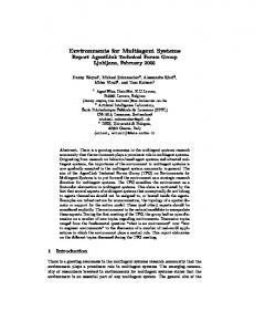
We introduce the Packet-World application we have developed (Weyns and Holvoet, 2002), since this is used as an example MAS throughout the text. The Packet-World consists of a number of different colored packets that are scattered over a rectangular grid. Agents that live in this virtual world have to collect those packets and bring them to their corresponding colored destination. The grid contains one destination for each color. Figure 1 shows an example of a Packet-World with size 10 wherein 5 agents are situated. Squares symbolize packets and circles are delivery points. The colored rings symbolize pheromone trails discussed below. In the Packet-World, agents can interact with the envi-

ronment in a number of ways. We allow agents to perform a number of basic actions. First, an agent can make a step to one of the free neighbor fields around him. Second, if an agent is not carrying any packet, it can pick one up from one of its neighboring fields. Third, an agent can put down the packet it carries on one of the free neighboring fields around it, which could of course be the destination field of that particular packet. It is important to notice that each agent of the PacketWorld has only a limited view on the world. This view only covers a small part of the environment around the agent (see figure 1). Furthermore, agents can interact with other agents too. We allow agents to communicate indirectly using stygmergy (Sauter et al.; Parunak and Brueckner, 2000; Brueckner, 2000): agents can deposit pheromone-like objects at the field they are located on. These pheromones evaporate over time and can be perceived by other agents. In the Packet-World, this allows agents to construct pheromone trails between clusters of packets and their destination (Steels, 1990). In figure 1 pheromones are symbolized by colored rings. The color of the ring corresponds to the packet color. The radius of the ring is a measure for the strength of the pheromone and decreases as the pheromone evaporates. Other agents noticing a pheromone trail can decide to follow it in the direction of increasing pheromone strength to get to a specific destination (e.g. when they are already carrying a packet of corresponding color). On the other hand, agents can also decide to follow the trail in the direction decreasing pheromone strength leading to the packet cluster (e.g.

Figure 1: The Packet-World: global screenshot (left) and view range of agent nr.4 when they are not carrying anything). Hence they can help transporting the clustered packets, while reinforcing the evaporating pheromone trail on their way back to the destination. In this way stygmergy provides a means for coordination between the agents which goes beyond the limitations of the agents’ locality in the environment.

1.2

Problem Statement

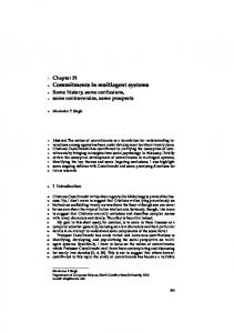
So far, time in MASs is generally dealt with in an implicit and ad hoc way: once the agents have been developed, they are typically hooked together using a particular activation regime or scheduling algorithm (see figure 2), without decent time management. MASs with an implicit notion of time are generally not adapted at all to run-time variations of timing delays introduced by the underlying execution platform, e.g. network delays, delays due to scheduling policies, etc. Moreover, these variations with respect to the execution of the agents can have a severe impact on the behavior of the MAS as a whole (Axtell, 2000; Page, 1997). The reason for this is that mostly the temporal relations existing in the problem domain differ significantly from the arbitrary and variable

Figure 2: MAS directly built upon an execution platform

time relations in an execution platform (Fujimoto, 1998), emphasizing the need for an explicit time management. In other words, delays in an execution platform are based on quantities which have nothing to do with the problem domain. To illustrate this, consider the following examples from our Packet-World application: 1. From the MAS’s point of view, agents with simpler internal logic are expected to react faster than agents with more complex internal logic. However, consider a packet lying in between a cognitive agent and a significantly faster reactive agent, for instance the white packet between agents 2 and 3 in figure 1. In case both agents start reasoning at the same time, it seems obvious that the reactive agent can pick up the packet before the cognitive one can. However in practice, the response order of both agents is arbitrary, because the underlying execution platform could cause the cognitive agent’s process to be scheduled first, allowing it to perform its reasoning and pick up the packet before the faster reactive agent even got a chance. 2. The agents can deposit pheromones drops in the environment to coordinate their activity. These pheromones evaporate over time. Because the effectiveness of pheromone-based communication is strongly dependent upon this evaporation rate, the latter is tuned to suit the needs of a particular application. However, fluctuations in the load of the underlying execution platform can cause agents to speed up or slow down accordingly, leading to a significant loss of pheromone effectiveness which affects the overall behavior of the MAS. 3. Problems can also arise with respect to the actions agents can perform. In our Packet-World applica-

tion the time period it takes to perform a particular action must be the same for all agents. However, fluctuations in processor load can introduce variabilities with respect to the execution time of actions. As a consequence a particular action of an agent can take longer than the same action performed by other agents. This leads to agents arbitrarily obtaining privileges compared to other agents due to the execution platform, a property which is undesired in our problem domain. The examples above show that a MAS without explicit time management is not adapted to varying delays introduced by the execution platform, which can be the cause of unforeseen or undesired effects. Hence the execution of all entities within a MAS has to be controlled according to the requirements at the level of the MAS, irrespective of execution platform delays. In this paper, we introduce time management adaptability as a generic solution to this problem and a more structured way to control the execution of a MAS. Figure 3: Time management adaptability in MASs

1.3

Time Management Adaptability

Time management adaptability allows the execution of a MAS to be controlled by ensuring that all temporal relations which are essential from a conceptual point of view are correctly reproduced in the software system. Hence a particular execution policy for each MAS can be enforced. Second, time management adaptability allows easy adaptation of a MAS’s execution, because it deals with time in an explicit manner and introduces execution control into a MAS as a separate concern. In order to achieve this, time management adaptability consists of three main aspects (see figure 3): 1. Time models are necessary to explicitly model the way time considered in the problem domain, without taking into account the underlying execution platform. Hence time models capture time at level of the MAS application. Time models are explicit which allows them to be easily adapted to reflect the custom needs of a MAS application. 2. Time management mechanisms are a means to ensure the consistency of time as being defined at the MAS level, even in the presence of arbitrary delays introduced by the execution platform. 3. A MAS execution control platform combines both time models and time management mechanisms to control the execution of a MAS. In a MAS execution control platform time models are used to capture the execution requirements and time management mechanisms are employed to prevent time models from being violated during execution. In this way the conceptual perception of time can be decoupled from the timing delays of the platform on which the MAS executes.

Outline of the paper. We first clarify the concept of time in MASs in section 2. We then discuss the various parts of time management adaptability: in section 3 we elaborate on time models. In section 4, the main time management mechanisms existing today are evaluated, and section 5 discusses MAS execution control platforms more in detail. Finally, we look forward to future work in section 6 and conclude in section 7.

2 2.1

Time in MAS Causality And Time

Time in MASs is important because it determines causality (Schwarz and Mattern, 1994). To illustrate this, we start from the fundamental characteristics of MASs, as stated in the definition of Wooldridge and Jennings: “an agent is a computer system that is situated in some environment, and that is capable of autonomous action in this environment in order to meet its design objectives” (Wooldridge and Jennings, 1995). Agents are not isolated entities, but instead they are situated in an environment which they can perceive and on which they can act. By means of this shared environment, the actions of one agent have an influence on other agents. The order in which the actions take place in the environment determines the actual causality between agents. We now elaborate on what causes a particular ordering of actions to arise and hence what actually determines causality in MASs. By means of coordination, agents can agree upon the order. However, to see what is determining the order in the absence of coordination, we return to the autonomy property of individual agents:

agents autonomously decide when to perform an action. Therefore in MASs, no global flow of control can be identified which unambiguously determines causality. Instead, each agent has its own, local flow of control. As a consequence, in the absence of explicit coordination between agents, the relative timing between their corresponding local control flows determines in which order their actions on the environment happen. We conclude that in MASs, time determines causal dependencies between non-coordinating agents.

2.2

Different Concepts of Time

One of the most common points of confusion is what is actually meant by time in software systems. We start from (Fujimoto, 1998) to distinguish 2 sorts of time which are of relevance for the rest of the paper: • Wallclock time is the (execution) time as measured on a physical clock while running the software system. For example, in the Packet-World the execution of a particular agent to determine its next action might take 780 milliseconds on a specific processor. • Logical time (also called virtual time) is the software representation of time as experienced in the problem context. For example, the current logical time of our application could be represented by an integer number; after executing the program for 37 minutes of wallclock time, 892 units of logical time may have passed. According to the way logical time advances in a system, a number of execution modes can be distinguished (Fujimoto, 1998). In a real-time execution, logical time advances in synchrony with wallclock time. Here we are mainly concerned with as fast-as-possible executions, which attempt to advance logical time as quickly as possible, without direct relationship to wallclock time. As an example: for a software system it could be that after 5 minutes of wallclock time, 100 units of logical time may have been processed, while after 10 minutes of execution time, 287 logical time units have passed in an as fast as possible execution, instead of 200 for real-time execution.

3

Time Models

Time models are inspired by research in the distributed simulation community, where they are used implicitly to assign logical time stamps to all events occurring in the simulation (Lamport, 1978; Misra, 1986). In software simulations, the logical time stamp of an event corresponds to the physical time the event was observed in the real world which is being simulated. However, we extend the use of time models from pure simulation contexts to execution control for MASs in general. Here, logical time is not used to obtain correspondence to physical time, which has no meaning outside the

Figure 4: A typical agent control flow cycle scope of simulation, but as a means to express causality in a MAS (see section 2.1). Also in contrast to software simulations, time models are now explicitly represented, which allows them to be easily adapted. A time model captures the requirements with respect to time, as exposed in the problem context of most applications. More precisely, a time model defines how the duration of various activities in a MAS is related to logical time, and the order of activities in logical time is used as a means to express causality between the entities in a MAS. In this way a time model allows the developer to describe the causal relationships which are essential for the correct working of the MAS and hence must be ensured during the execution of the MAS on any particular platform. Time models capture time relations at the level of the MAS’s problem domain. A first important thing which needs to be done when considering time models, is investigating the structure of a MAS to identify all entities that need to be time modeled.

3.1

Time Modeling Agents

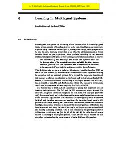
In the previous section we stated that time determines causal relations between agents, since each of the latter has its own control flow. Hence the first important MAS entities which require time modeling are the agents. Because generally agents can perform several activities, time modeling an agent requires assigning durations in logical time to all of its activities. For our discussion, we assume that an agent has a control flow cycle as the one depicted in figure 4. 3.1.1

Agent deliberation

A first important activity an agent can perform, is internal deliberation. The purpose of this activity is determining the next action the agent is going to perform. Depending on the context, agent’s deliberation can be very simple (e.g. stimulus-response behavior in reactive agents) or

immensely complex (e.g. sophisticated learning and planning algorithms used in cognitive agents). In the context of agent-based simulation, time modeling agent’s deliberation has received a lot of interest. We evaluate various time models which have been proposed to describe how much logical time the deliberation of the agents takes, and discuss their relevance for execution control. • A constant time model (Uhrmacher and Kullick, 2000) for the agents’ deliberation implies that the deliberation of all agents is performed in a constant logical time, irrespective of the actual wallclock time that is needed to execute the deliberation. By assigning constant logical time durations to the deliberation activity of each agent, one can determine the relative speed of all agents within a MAS at conceptual level, irrespective of their implementation or execution efficiency. • If the functionality of an agent has to be time sensitive, a model assuming that the agent’s deliberation always happens in a constant logical duration is no longer suitable. In this case, the logical duration of the deliberation activity can be modeled as a function of reasoning primitives (Anderson, 1997), e.g. evaluating the results of a perception action, updating its internal world model, etc. In this case, deliberation time cannot be predicted a priori, because only those primitives which are actually used during a particular deliberation phase are taken into account to determine the duration in logical time. However, although this approach is conceptually feasible, it requires zooming in into the agent’s internal working to monitor what the agent is actually deliberating about. • A popular approach uses the actual computer instructions as a basis for determining the logical deliberation time. At first sight, modeling the logical deliberation time of an agent as a function of the number of code instructions executed during deliberation could be considered an extreme example of the previous approach which treats each computer instruction as a reasoning primitive (Anderson, 1997). However counting computer instructions is related to the underlying execution platform rather than to the conceptual level of the MAS. Hence precaution has to be taken when using it in a time model for execution control, since this approach can cause a number of unexpected effects to occur. Using this model, the programming language used for an agent, the efficiency of implementation and the presence of GUI or debug code have a significant influence on the logical deliberation time, although these aspects have no conceptual meaning. Another drawback of this approach is that a “timed” version of the language in which the agents are programmed is required, e.g. Timed Common Lisp.

• The logical deliberation time can be modeled as a function of the wallclock time used for executing the deliberation (Anderson, 1995). This approach is also not feasible from conceptual point of view, since the logical duration is now susceptible to the load and performance of the underlying computer system. 3.1.2

Agent Action

A second important activity of an agent is performing actions (see figure 4). Compared to agent deliberation, time modeling agents’ actions on the environment has received little interest. However, in the context of execution control, imposing time models on the actions agents perform is indispensable. Depending on the problem context, actions can be assigned a particular cost expressed as a time penalty the agent receives for performing the action. From the agents’ point of view, this period of logical time can be considered as the time the agent needs to complete that particular action. Since meanwhile the agent is not allowed to perform anything else, this approach can be used to model the frequency an agent is allowed to perform actions, irrespective of the underlying execution platform. 3.1.3

Agent Perception

Agent perception is also an agent activity which must be time modeled, however this is often neglected. Assigning a logical time duration to perceptual actions is analogous to time modeling other actions. An advantage of time modeling perception is for example that it can be a means to better control agents which continuously poll the environment by means of perception.

3.2

Time Modeling Ongoing activities

Besides the agents, there can be other entities within a MAS which require time modeling. In MASs, there is an increased environmental awareness. The environment itself is often dynamic and evolves over time. As a consequence causal relations do not only occur between interacting agents: the environment itself can contain a number of ongoing activities which are essential for the correct working of the MAS as a whole (Parunak et al., 2001). Ongoing activities are characterized by a state which evolves over time, even without agents affecting it. Agents can often initiate ongoing activities and influence their evolution. For example a ball in a robocup soccer game that was kicked by an agent, or the pheromones in our Packet-World application which evolve continuously. We conclude that the environment is not passive, but active, and responsible for the evolution of all ongoing activities. In many MAS applications however, the dynamics of ongoing activities are dealt with in an ad hoc way. For example, the evaporation rate of pheromones is modeled in wallclock time, such that the correlation between agent activity on the one hand and pheromone activity

on the other hand is not guaranteed. As a consequence optimal coordination effectiveness can hardly be maintained: varying loads on the execution platform cause agent activity to slow down or speed up accordingly, while pheromone evaporation is determined upon wallclock time and hence not adaptive to platform loads. Therefore it is very useful to provide ongoing activities of the environment with a time model, which allows their activity to be controlled to suit the needs of the MAS application.

3.3

Time Models: A Case

We now return to the Packet-World application, and illustrate the use of time models to capture the causal relations which are necessary for the correct working of the MAS and hence must be ensured on any particular platform. The problem statement (see section 1.2) mentions a number of typical problems with respect to execution control which arise in our Packet-World application. We now elaborate on describing the requirements in our problem examples to derive time models. In the Packet-World, the following actions can be distinguished: a move action, a pick up packet action, a put packet down action and a drop pheromone action. Stated formally: E = {move, pick, put, drop} with move = move action pick = pick up packet put = put down packet drop = drop pheromone With E the set of all possible actions on the environment. In our application, there is only one perceptual action: agents can see their neighborhood. Formally: P = {look} with look = visual perception With P the set of perceptual actions. We distinguish two types of agents in our PacketWorld: reactive agents and cognitive agents. Each agent is either reactive or cognitive. Stated formally: AR = {ar1 , ar2 , ..., arn } AC = {ac1 , ac2 , ..., acm } A = AR

S

AC = {a1 , a2 , ..., am+n }

With AR the set of all reactive agents in our Packet-World application, AC the set of all cognitive agents, and A the set of all agents, reactive and cognitive.

3.3.1

Action Requirements

We take a closer look at the third problem mentioned in section 1.2. In our Packet-World application it was observed that the the underlying execution platform can have an arbitrary influence on the time it takes to perform an action. However, in the problem domain it is required the same amount of time is needed for all agents to perform a particular action. Stated formally: ∀ai ∈ A; move, pick, put, drop ∈ E : ∆Tact (move, ai ) = cstmove ∆Tact (pick, ai ) = cstpick ∆Tact (put, ai ) = cstput ∆Tact (drop, ai ) = cstdrop cstmove , cstpick , cstput , cstdrop ∈ ℵ With A the set of all agents, E the set of all actions on the environment, ∆Tact (e, ai ) the logical duration of action e performed by agent ai , and ℵ the set of natural numbers. The previous equations can also be expressed as: ∀ai ∈ A; ∀e ∈ E : ∆Tact (e, ai ) = cste cste ∈ ℵ Since perception is considered as a kind of action in our application, we obtain the following expression: ∀ai ∈ A; look ∈ P : ∆Tper (look, ai ) = cstlook cstlook ∈ ℵ With A the set of all agents, P the set of all perceptual actions, ∆Tper (look, ai ) the logical duration of perceptual action look performed by agent ai , and ℵ the set of natural numbers. Stated more generally: ∀ai ∈ A; ∀p ∈ P : ∆Tper (p, ai ) = cstp cstp ∈ ℵ

3.3.2

Deliberation Requirements

We now return to the first example of our Packet-World application. The problem was the fact that the underlying execution platform can influence the reaction speed of the agents, leading to a response order which is arbitrary. However, this is not desired from a conceptual point of view, where we would like the reactive agent to always react faster than the cognitive agent, in case both start deliberating at the same time. Based on an agent’s control flow cycle as depicted in figure 4, the moment in logical time an agent completes an action can be stated formally

as: ∀ai ∈ A; ∀e ∈ E; look ∈ P : Tend (e, ai ) = T0 + ∆Tper (look, ai ) + ∆Tdelib (ai ) + ∆Tact (e, ai ) With Tend (e, ai ) the logical time the action e of agent ai completes, T0 the logical time that a new cycle in the control flow of agent ai starts, ∆Tper (look, ai ) the logical duration of the perception look performed by agent ai , ∆Tdelib (ai ) the logical duration of the deliberation of agent ai , and ∆Tact (e, ai ) the logical duration of action e performed by agent ai . The requirement that reactive agent can always pick up the packet before cognitive agent in case both start deliberating at the same time, is hence formalized as follows: ∀ari ∈ AR ; ∀acj ∈ AC ; pick ∈ E : Tend (pick, ari ) < Tend (pick, acj ) With AR the set of reactive agents, AC the set of cognitive agents, and E the set of all actions on the environment. By substitution we obtain: T0 + cstlook + ∆Tdelib (ari ) + cstpick T0 + cstlook + +∆Tdelib (acj ) + cstpick