An interpolation algorithm usually consists of two phases: velocity planning and parame- ter computation. ... needed and used a constant feedarte in other places [23]. However, the ... Furthermore, all these methods are not proved to be time-optimal. ... algorithm in CNC machining under the same acceleration constraints.
Mathematics Mechanization Research Preprints KLMM, Chinese Academy of Sciences Vol. 29, 165–188, September 2010
165
Time-Optimal Interpolation of CNC Machines along Parametric Path with Chord Error and Tangential Acceleration Bounds Chun-Ming Yuan, Xiao-Shan Gao KLMM, Institute of Systems Science, Chinese Academy of Sciences E-mail: (cmyuan,xgao)@mmrc.iss.ac.cn. Abstract. Interpolation and velocity planning for parametric curves are crucial problems in CNC machining. In this paper, a time-optimal velocity planning algorithm under a given chord error bound and a tangential acceleration bound is proposed. The key idea is to reduce the chord error bound to a centripetal acceleration bound which leads to a velocity limit curve, called the chord error velocity limit curve (CEVLC). Then, the velocity planning is to find the time-optimal velocity curve governed by the tangential acceleration bound “under” the CEVLC. For two types of simple splines, explicit formulas for the optimal velocity curve are given. We implement the methods in these two cases and use curved segments from real machining parts to show the feasibility of the methods. Keywords. Parametric curve interpolation, time-optimal velocity planning, chord error, velocity limit curve.
1
introduction
In modern CAD systems, the standard representation for free form surfaces is parametric functions. While the conventional computed numerically controlled (CNC) systems mainly use micro line segments (G01 codes) to represent the machining path. To convert the parametric curves into line segments is not only time consuming but also leads to problems such as large data storage, speed fluctuation, and poor machining accuracy. In the seminal work [5, 18, 22], Chou, Yang, and Shpitalni et al proposed to use parametric curves generated in CAD/CAM systems directly in the CNC systems to overcome these drawbacks. An interpolation algorithm usually consists of two phases: velocity planning and parameter computation. Let C(u) be the manufacturing path. The phase to determine the feed-rate v(u) along C(u) is called velocity planning. When the feed-rate v(u) is known, the way to compute the next interpolation point at ui+1 = ui + 4u during one sampling time period is called parameter computation. This paper focuses on velocity planning along a spatial parametric path. For the parameter computation phase, please refer to [4, 9, 21] and the literatures in them. Two types of acceleration modes can be used in the velocity planning: the tangential acceleration and the multi-axis acceleration where each axis accelerates independently. Due to its conceptual simplicity, the tangential acceleration is widely used in CNC interpolations. Bedi et al[1] and Yang-Kong[22] used a uniform parametric feed-rate without
166
C.M. Yuan and X.S. Gao
considering the chord error. Yeh and Hsu used a chord error bound to control the feed-rate if needed and used a constant feedarte in other places [23]. However, the machine acceleration capabilities were not considered. Narayanaswami and Yong [24] gave a velocity planning method based on tangential acceleration bounds by computing maximal passing velocities at sensitive corners. Cheng and Tsai [4] gave an interpolation method based on different velocity profiles for tangential ACC/DCC feed-rate planning. Velocity planning methods with tangential acceleration and jerk bounds were considered by several research groups [7, 11, 13, 14, 12]. In particular, Emami and Arezoo [6], Lai et al[10] proposed velocity planning methods with confined acceleration, jerk, and chord error constraints by checking these values at every sampling point and using backtracking to adjust the velocity if any of the bounds is violated. In all the above methods besides [6, 10, 23], the chord error is considered only at some special points, and there is no guarantee that the chord error is satisfied at all points. Furthermore, all these methods are not proved to be time-optimal. In the multi-axis acceleration case, Borow [3] and Shiller et al [16, 15] presented a timeoptimal velocity planning method for a robot moving along a curved path with acceleration bounds for each axis. Farouki and Timar [19, 20] proposed a time-optimal velocity planning algorithm in CNC machining under the same acceleration constraints. Following the method in [19, 20], Zhang et at gave a simplified time-optimal velocity planning method for quadratic B-splines and realized real-time manufacturing on industrial CNC machines [26]. Zhang et al[25] gave a greedy algorithm for velocity planning under multi-axis jerk constraints. These optimal methods use the “Bang-Bang” control strategy, that is, at least one of the axes reaches its acceleration bound all the time. But they do not consider the chord error which is an important factor for CNC-machining. In this paper, we give a time-optimal velocity planning algorithm along a parametric curve path C(u) under a given chord error bound and a tangential acceleration bound. The main contribution of the paper is the introduction of the chord error velocity limit curve (abbr. CEVLC) and the velocity planning algorithm. We show that the chord error bound can be approximately reduced to a centripetal acceleration bound. Furthermore, if the centripetal acceleration reaches its maximal bound, the velocity can be written as an algebraic function in the parameter u of the curve path C(u). The graph of this function is called the CEVLC. The CEVLC is significant because the final velocity curve must be “under” this curve or be part of this curve, which narrows the range of velocity planning. Also, certain key points on the CEVLC, such as the discontinuous points, play an important role in the velocity planning. Similar to the previous work on time-optimal velocity planning, our algorithm also uses the “Bang-Bang” control strategy, which is a necessary condition for time optimal in our case. Then the final velocity curve is governed either by the centripetal acceleration bound or by the tangential acceleration bound, and the later one is called the integration velocity curve. The main task of the velocity planning is to find the switching points between the integration velocity curve and the CELVC. Two main results on the optimal velocity curve are given in this paper. Firstly, as a theoretical result, we show that the final velocity is the minimum of the CEVLC and all the integration velocity curves passing through the initial point, the termination point, and the key points of the CEVLC. We also give a practical algorithm to compute the optimal
Time-Optimal Control of CNC Machines with Chord Error
167
velocity curve incrementally. For quadratic splines and cubic PH curves, the integration velocity curve can be given by explicit formulas. We implement our algorithm in these two cases and conduct experiments using curved pathes from real manufacturing parts. Moreover, we also give a simple and real-time feed-rate override algorithm based on our velocity planning curve. For multi-axis velocity planning algorithms, feed-rate override is complicated and not suitable for real time interpolation. As a final remark, we want to mention that by combining the CEVLC proposed in this paper and the method proposed in [19, 20], it is possible to give a time optimal velocity planning method under a given chord error bound and multi-axis acceleration bounds. The rest of the paper will be organized as follows. Section 2 gives the time-optimal velocity planning algorithm for a parametric curve. Section 3 gives the details for computing the time optimal velocity curves for quadratic B-spline and cubic PH-spline. Section 4 gives a feed-rate override algorithm for CNC-machining. Section 5 concludes the paper.
2
Time-optimal velocity planning under chord error and tangential acceleration bound
The time-optimal velocity planning algorithm will be presented in this section. We consider a spatial piecewise parametric curve C(u), u = 0..1 with C 1 continuity, such as splines, Nurbs, etc. We further assume that each piece of the curve is differentiable to the third order and has left and right limitations at the endpoints.
2.1
Problem
In order to control the machine tools, we need to know the velocity of the movement at each point on the curve, which is denoted as a function v(u) in the parameter u and is called the velocity curve. The procedure to compute the velocity curve v(u) is called velocity planning. In this subsection, we will show that the chord error bound can be reduced to the centripetal acceleration bound and formulate the velocity planning problem as an optimization problem with tangential and centripetal acceleration bounds. For a parametric curve C(u), we denote its parametric speed to be: σ(u) =
ds = |C 0 (u)|, du
where 0 is the derivative w.r.t. u. The curvature and radius of curvature are defined to be: k(u) =
|C 0 (u) × C 00 (u)| 1 , ρ(u) = . 3 σ(u) k(u) P Q
|PQ|: chord error
Fig. 1.
The chord error
168
C.M. Yuan and X.S. Gao
The cutter moves in a line segment between two adjacent points on the curve C(u) and the distance between the line segment and the curve segment is called the chord error which is the main source of the manufacturing error (Fig 1). Firstly, we will show that the chord error bound can be reduced to the centripetal acceleration bound. Let T be the sampling period, δ the error constraint, and ±A the tangential acceleration bounds. In practice, the chord error bound is much less than the radius of curvature at each point on the curve. By the chord error formula [23], at each parametric value u, q(u) = v 2 (u) ≤
8δρ(u) − 4δ 2 8δρ(u) 8δ ≈ = . 2 2 T T k(u)T 2
If we denote by d(u) the interpolating chord error at u with feed-rate v(u), then d(u) = ≤ δ. Let
T 2 v(u)2 8ρ(u)
aN (u) = v(u)2 /ρ(u) = k(u)v(u)2 = k(u)q(u)
(1)
be the centripetal acceleration and
8δ . T2 Then, the chord error bound is transformed to the centripetal acceleration bound: B=
(2)
d(u) ≤ δ ⇐⇒ aN (u) ≤ B. Since
d ds du d v d = = , dt dt ds du σ du
(3)
The tangential acceleration is: aT (u) =
dv(u) v(u)v 0 (u) q 0 (u) = = . dt σ(u) 2σ(u)
(4)
From (3), the time optimal velocity planning problem becomes the following optimization problem: to find a velocity curve v(u) such that Z min t = v(u)
0
1
σ(u) du, v(u)
(5)
with the tangential and centripetal acceleration constraints |aT (u)| ≤ A, aN (u) ≤ B, u = 0..1,
(6)
where (aT (u), aN (u)) are the tangential and centripetal accelerations and (A, B) are their bounds respectively. Note that B can be derived from the chord error bound from (2).
Time-Optimal Control of CNC Machines with Chord Error
2.2
169
The main result
In this section, we present the main result of the paper about the time optimal velocity planning problem (5). We will give a velocity planning algorithm in section 2.4 and prove the correctness of the result in section 2.5. Before giving the main result, we need to introduce several basic concepts. We use “Bang-Bang” control, that is, at least one of “=” holds among the inequalities in (6). This will lead to two cases. B , If the centripetal acceleration reaches its bound B, then from (1) we have q(u) = k(u) which defines a curve 2 qlim (u) = vlim (u) = B/k(u), u ∈ [0, 1] or p vlim (u) = B/k(u), u ∈ [0, 1],
(7)
in the u-v plane with v as the vertical axis. We call this curve the velocity limit curve with the chord error constraint, denoted by CEVLC. If C(u) is a piecewise curve with C 1 continuity, then its CEVLC is the combination of the CEVLCs of its components. From the constraint aN ≤ B, the velocity curve must be “under” the CEVLC in the v direction. 2
2u 1−u Example 2.1 If C(u) = ( 1+u 2 , 1+u2 , 0) and B = 100, then vlim (u) = 10, u ∈ [0, 1].
3
If C(u) = (u2 +u+1, u2 +2u−1, 2u+1) and B = 600, then vlim (u) = 10(8u2 +12u+9) 4 , u ∈ [0, 1]. If C(u) = ( 13 u3 − 4u2 − 8u, 23 u3 + 3u2 − 8u, − 32 u3 − 2u2 − 14u) and B = 1000, then vlim (u) = 30u2 + 40u + 180, u ∈ [0, 1]. If the tangential acceleration reaches its bound, then from (4) the square of the velocity q(u) = v(u)2 can be obtained by solving the differential equation q 0 (u) = ±2Aσ(u), whose solution is q = ±2Aπ(u) + c, (8) R where π(u) = σdu is the primitive function of σ(u) and c a constant which can be determined by an initial point (u∗ , q(u∗ )): c = q(u∗ ) ∓ 2Aπ(u∗ ). The curve (8) is called the integration curve or the integration trajectory. Let vP (u) be the integration trajectory with tangential acceleration A starting from an initial point P = (uP , vlim (uP )) both for the forward (the +u) and the backward (the −u) directions. Let v0 (u) be the forward integration trajectory with tangential acceleration A from the initial point P0 = (0, 0) and v1 (u) the backward integration trajectory with tangential acceleration A from the initial point P1 = (1, 0). Of curse, all the curves mentioned above are defined in [0, 1]. Then, the solution to the optimization problem (5) is given below. Theorem 2.2 Let K be the finite set of key points of the CEVLC to be defined in the next section. Then v(u) = min(vlim (u), vP (u), v0 (u), v1 (u)). (9) P ∈K
Then, v(u) is the solution to the optimal problem (5).
170
C.M. Yuan and X.S. Gao
Obviously, v(u) is a piecewise continuous curve for u ∈ [0, 1]. We will prove the theorem in Section 2.5.
2.3
Key points of the CEVLC
There exist three types of special points on the CEVLC, which are called switching points or key points. The first type switching points are the discontinuous points of the CEVLC. These points correspond to the curvature discontinuous points of the original curve. They must be the singular points of the parametric curve or the connection points of two curve segments. If we denote by C(u) the curve segment, then the singular points of C(u) can be computed by solving the equations C 0 (u) × C 00 (u) = 0. From (7), the limit velocity vlim is ∞ at these points and the real velocity curve can not reach it, so we can omit the singular points from the key points. Thus, only the connection points need to be considered. At a first type key point, the velocity is not continuous and we call the smaller one of the left and right side velocities as the minimal velocity or simply the velocity of this point. The second type switching points are the continuous but non-differentiable points of the CEVLC (slope discontinuity). These points correspond to the curvature continuous but nondifferentiable points of the original curve. Hence, they must be the connection points of two curve segments. For a differentiable segment of the CEVLC divided by the above two types of key points, we can divide it according to whether the tangential acceleration of the CEVLC is ±A, where A is from (6). A point on the CEVLC is called a key point of the third type if the tangential acceleration along the CEVLC at this point is ±A. We can find the third type key points by solving the following algebraic equation in u aT (u) =
qlim (u) Bσ(u)2 = = ±A. 2σ(u) 2|C 0 (u) × C 00 (u)|
With these switching points, the CEVLC is divided into two types of segments: 1. A curve segment is called feasible if the absolution values of tangential acceleration at all points are bounded by A. A feasible CEVLC segment can be a part of the final velocity curve. 2. A curve segment is called unfeasible if the absolution values of tangential acceleration at all points are larger than A. An unfeasible CEVLC segment cannot be a part of the final velocity curve. In other words, the final velocity curve must be strictly under it. If the curve segments on the left and right sides of a second type key point are both feasible, we delete this key point.
2.4
The time optimal velocity planning algorithm
We use the “Bang-Bang” control strategy. Then the real velocity curve is governed either by the maximal centripetal acceleration or by the maximal tangential acceleration. Since the velocity curve must be under or be a part of the CEVLC, we need to find the proper
Time-Optimal Control of CNC Machines with Chord Error
171
integration trajectory under the CEVLC. We first give the main idea of the velocity planning algorithm. Firstly, we compute the CEVLC, find the key points and their speeds. Compute the forward integration trajectory vs from the starting point (0, 0) with tangential acceleration A. Find the intersection point (ul , vs (ul )) of vs and the CEVLC. Compute the backward integration trajectory ve from the ending point (1, 0) with tangential acceleration A. Find the intersection point (ur , ve (ur )) of ve and the CEVLC. Secondly, if (ul , vs (ul )) = (ur , ve (ur )), then return the combination of vs and ve as the final velocity curve. If ul > ur , find the intersection point of vs and ve and return the combination of vs and ve as the final velocity curve. Otherwise, set Pc = (ul , vs (ul )) to be the current point and consider the following three cases. If the next segment of CEVLC from point Pc in the forward direction (the +u direction) is feasible, then we merge this feasible segment into vs and set the current point (ul , vs (ul )) to be the end point of this segment. If the next segment of CEVLC from point Pc in the forward direction is not feasible and the forward integration trajectory vf with initial point Pc is under the CEVLC, then let (ui , vf (ui )) be the intersection point of vf and the CEVLC. Merge vf (u), u ∈ [ur , ui ] into vs . Let ul = ui and Pc = (ul , vf (ul )). If the next segment of CEVLC from point Pc in the forward direction is not feasible and the integration trajectory vf with initial point Pc is above the CEVLC, then we find the next key point Pn on the right hand side of Pc . From Pn , compute the backward integration trajectory vb , find the intersection point of vb with vs , and merge vb and vs as the new vs . Set Pn as the new current point. Finally, with the new current point, we can repeat the procedure from the second step until the velocity curve is found. Here by saying a forward curve v1 (u) is under or above another curve v2 (u) from a point P = v1 (u∗), we mean that v1 (u) is under or above v2 (u) in a neighborhood of u∗ in the forward direction. To describe our algorithm precisely, we need the following notations. For a discontinuous curve f1 (x), we denote by f1+ (x∗ ) and f1− (x∗ ) the limitations of f1 (x) at x∗ from the left and right hand sides respectively, and define f1 (x∗ ) = min(f1+ (x∗ ), f1− (x∗ )). Let f2 (x) be a curve with C 0 continuity. If f2 (x∗ ) = f1 (x∗ ) or f2 (x∗ ) is between the left and right limitations of f1 (x) at x∗ , then define (x∗ , f2 (x∗ )) to be the intersect point of the curves (x, f2 (x)) and (x, f1 (x)). We now give the velocity planning algorithm. Algorithm VP CETA. The input of the algorithm is the curve C(u), u ∈ [0, 1], a chord error bound d, and a tangential acceleration bound A. The output is the velocity curve vc (u), u ∈ [0, 1] which is the solution to the optimization problem (5). 1 Compute the CEVLC in (7) and its key points as shown in section 2.3. Denote by Uf the parametric intervals where the corresponding segments of the CEVLC are feasible. 2 From the starting point (0, 0), compute the forward integration trajectory vs using the tangential acceleration A. Compute the first intersection point (ul , vs (ul )) of vs and the CEVLC. If there exists no intersection, denote ul = 1.
172
C.M. Yuan and X.S. Gao
3 From the ending point (1, 0), compute the backward integration trajectory ve using the tangential acceleration A. Compute the first intersection point (ur , ve (ur )) of ve and the CEVLC. If there exists no intersection, denote ur = 0. 4 If (ul , vs (ul )) = (ur , ve (ur )), then return the combination of vs and ve as the final velocity curve. If ul > ur , find the intersection point (ui , vs (ui )) of vs and ve , return v(u), where ( vs , 0 ≤ u ≤ ui v(u) = (10) ve , ui < u ≤ 1. 5 If (ul , vlim (ul )) is a discontinuous point on the CEVLC, there are three possibilities. + − (a1) If vlim (ul ) > vs (ul ) = vlim (ul ), goto step 6. + − (a2) If vlim (ul ) = vs (ul ) < vlim (ul ), goto step 8. + − (a3) If vlim (ul ) ≥ vs (ul ) > vlim (ul ), let un = ul and goto step 9.
6 Now, (ul , vs (ul )) is the starting point of the next segment of CEVLC. There exist three cases. (b1) If the next segment of the CEVLC is feasible, goto step 7 (b2) If a− T (ul ) ≥ A, goto step 8. (b3) If a− T (ul ) ≤ −A, then find the next key point (un , vlim (un )) along the +u direction and goto step 9. 7 Let un > ul be the parameter of the next key point. Then, (ul , un ) ⊂ Uf . Update vs to be ( vs (u), 0 ≤ u < ul vs (u) = vlim (u), ul ≤ u ≤ un . Let ul = un , goto step 4.
vlim
vlim vlim vf
vf vlim
u=ul
(a) Case (a2) Fig. 2.
u=u l
(b) Case (b2)
Two cases of step 8: computation of forward integration curve
8 Starting from (ul , vs (ul )), compute the forward integration trajectory vf with tangential acceleration A. Find the first intersection point (ui , vf (ui )) of vf and the CEVLC (Fig. 2). If there exists no intersection, denote ul = 1. Update vs to be ( vs (u), 0 ≤ u < ul vs (u) = vf (u), ul ≤ u ≤ ui .
Time-Optimal Control of CNC Machines with Chord Error
173
vlim
vlim
vs vb
vs
vlim
vb u=un
u=un
(a) Case (a3) Fig. 3.
(b) Case (b3)
Two cases of step 9: computation of backward integration curve
Let ul = ui , goto step 4. 9 Starting from point (un , vlim (un )), compute the backward integration trajectory vb in the −u direction with tangential acceleration A. Find the intersection point1) (ui , vb (ui )) of vb and vs . See Fig. 3 for an illustration. Update vs to be ( vs (u), 0 ≤ u < ui vs (u) = vb (u), ui ≤ u ≤ un . Let ul = un , goto step 4. The correctness proof of the algorithm is given in Section 2.5. Further improvements of the algorithm are given in Section 2.6. The flow chart of the above algorithm is given in Fig. 5. The details of the algorithm is omitted in the figure. 110 100 100
80
90
II 80
VI
60
IV
70 V 40
VII
III
60 20
I
50
40
0 0
0.2
0.4
0.6
0.8
1
0.2
0.4
0.6
0.8
1
x
(a) CEVLC and key points Fig. 4.
(b) velocity curve
An illustrative example of velocity planning
Figure 4 is an illustrative example of the algorithm. Compute the CEVLC vlim and the key points as shown in Figure 4(a), where ◦ represents the key points of first type and the corresponding parameters are 0.2, 0.7; ¦ represents the key point of second type, and the corresponding parameter is 0.4; and ¤ represents the key points of third type. The gray parts are feasible segments. 1)
We will show that there exists a unique intersection point.
174
C.M. Yuan and X.S. Gao
Starting from point (u, v) = (0, 0), compute the forward integration trajectory vs which intersects the CEVLC at u = 0.2. Starting from (u, v) = (1, 0), compute the backward integration trajectory ve which intersects the CEVLC at u = 0.7. In step 5, the current point Pc is a discontinues point and case (a3) is executed. In step 9, starting from the first ◦ point, compute the backward integration trajectory vb which intersects vs at the first point marked by +. Update vs to be the piecewise curve marked by I, II in Figure 4(b). From the first point marked by ◦, the CEVLC is feasible. Hence, update vs to be the piecewise curve marked by I, II and the first gray part of the CEVLC(III). Let the key point marked by ¦ be the current point. From the current point, the CEVLC is not feasible and case (b3) is executed. In step 9, we select the next key point which is the first point marked by ¤. Starting from this point, compute the backward integration trajectory vb which intersects vs at the second point marked by +. Update vs to be the piecewise curve marked by I, II, III, IV in the figure. Starting from the first point marked by ¤, the CEVLC is feasible. Hence, update vs to be the piecewise curve marked by I, II, III, IV, V in the figure. Let the second point marked by ¤ to be the current point. Starting from this point, the CEVLC is not feasible and case (b2) is executed. In step 8, compute the forward integration trajectory vf which intersects ve at the third point marked by +. The final velocity curve consists of seven pieces marked by I, II, III, IV, V, VI, and VII in the figure. Note that the CEVLC can be parts of the final velocity curve quite often, while in [19, 20], the VLC is rarely a part of the final velocity curve. Remark 2.3 In the above algorithm, we need to compute the CEVLC and its key points, the integration trajectory, the intersection points of the integration trajectory and the CEVLC, and the intersection points of two integration trajectories. In principle, these computations can be reduced to computing integrations and solving algebraic equations. In Section 3, we will show how to give explicit formulas for the integration curve for two types of special types of curves.
2.5
The correctness of the algorithm
In this section, we will show that the velocity curve given by the algorithm in the preceding subsection is the only solution to the optimization problem (5). The proof is divided into two parts. We will first show that the velocity curve computed by the algorithm is the curve defined in (9) and then prove that this velocity curve is the solution to the problem (5). In order to prove this, we need the following result. Theorem 2.4 [2][p.24-26] Let y, z be solutions of the following differential equations y 0 = F (x, y), z 0 = G(x, z), respectively, where F (x, y) ≤ G(x, y), a ≤ x ≤ b, and F or G satisfies Lipschitz’s condition. If y(a) = z(a), then y(x) ≤ z(x) for any x ∈ [a, b]. In our case, the above theorem implies the following result.
Time-Optimal Control of CNC Machines with Chord Error
Fig. 5.
Flow chart of the velocity planning
175
176
C.M. Yuan and X.S. Gao
Lemma 2.5 Let v1 (u) and v2 (u) be two velocity curves for the curve C(u) and [u1 , u2 ] ⊂ [0, 1]. If v1 (u1 ) ≤ v2 (u1 ) and aT 1 (u) ≤ aT 2 (u) for u ∈ [u1 , u2 ], then v1 (u) ≤ v2 (u) for u ∈ [u1 , u2 ]. Furthermore, if v1 (u1 ) < v2 (u1 ), then v1 (u) < v2 (u) for u ∈ [u1 , u2 ]. Proof. We may assume that v1 (u1 ) = v2 (u2 ), since if v1 (u1 ) < v2 (u1 ), we may consider v¯2 (u) = v2 (u) − v2 (u1 ) + v1 (u1 ) which still satisfies the conditions in the lemma. Since C(u) is differentiable to the order of three, σ(u) and aT 1 (u) must be bounded in [u1 , u2 ]. From (4), q10 (u) = 2σ(u)aT 2 (u) and q20 (u) = 2σ(u)aT 2 (u). Then, we have q1 (u1 ) = v1 (u1 )2 = q2 (u1 ) = v2 (u1 )2 , 2σ(u)aT 2 (u) ≤ 2σ(u)aT 2 (u) for u ∈ [u1 , u2 ], and 2σ(u)aT 1 (u) satisfies the Lipschitz’s condition. Using Theorem 2.4, we have v1 (u) ≤ v2 (u) for u ∈ [u1 , u2 ]. The second part of the lemma can be proved similarly. Before giving the correctness proof, we first explain the key steps of the algorithm. Besides the in initial steps, new velocity trajectories are generated in Steps 7, 8, 9. We will show that these steps are correct in the sense that they will really generate new velocity trajectories. Step 7 is obvious, since we will use the next feasible CEVLC segment as the velocity trajectory. Two cases lead to step 8: cases (a2) and (b2). In case (a2), we have − + (ul ), which means there exists a parameter un > ul such that (ul ) = vs (ul ) < vlim vlim vlim (u) > vs (ul ) for u ∈ (ul , un ). As a consequence, starting at (ul , vs (ul )), we can use the tangential acceleration A to generate a piece of integration trajectory without violate the CEVLC (See Fig. 2(a)). In case (b2), there exists a parameter un > ul such that the tangential acceleration of the CEVLC must be strictly larger than A for u ∈ (ul , un ). By Lemma 2.5, starting from point (ul , vs (ul )), we can use the tangential acceleration A without violate the CEVLC (See Fig. 2(b)). We thus prove the correctness of step 8. The correctness step 9 can be proved in a similar way. Furthermore, we have Lemma 2.6 In step 9 of the algorithm, the backward integration trajectory vb intersects vs only once if there exist no overlap curve segments. Proof. Two situations lead to the execution of step 9: step (a3) and step (b3). In case − + (ul ). Then vs (ul ) ≥ vs (ul ) > vlim (a3), the key point at ul is of the first type and vlim and vb must intersect because vb decreasing with the acceleration −A and vs is bounded by ±A. By Lemma 2.5, vs and vc can intersects only once if there exist no overlap curve segments. Moreover, if there exists an overlap curve segment of vb and vs , then there exists no intersection point of vb and vs except the overlap curve segment by Lemma 2.5. Case (b3) can be proved similarly. Similarly, we can show that vs and ve in step 4 of the algorithm only intersect once if there exist no overlap curve segments. And we can use the bisection method to compute the intersection point. We now prove the main result of the paper. Theorem 2.7 The velocity curve computed with Algorithm VP CTEA is the velocity curve defined in equation (9) and is the only solution to the optimization problem (5). Proof. Let v(u) be the velocity curve computed with the algorithm. It is clear that v(u) is below the CEVLC and the tangential acceleration aT (u) of v(u) satisfies |aT (u)| ≤ A.
Time-Optimal Control of CNC Machines with Chord Error
177
Also, if |aT (u)| 6= A, the corresponding v(u) must be a segment of feasible CEVLC. As a consequence, v(u) satisfies conditions (6) and is bang-bang. From the algorithm, it is clear that v(u) consists of pieces of vP (u) for all key points P of the CEVLC including the start point (0, 0) and the ending point (1, 0). To prove (9), it suffices to show that for each key point P , if vP (u∗ ) 6= v(u∗ ) for a parametric value u∗ , then vP (u∗ ) > v(u∗ ). From the algorithm, it is clear that all key points including the starting and ending points are on or above v(u). Let P = (u0 , v0 ) be a key point. Then v0 ≥ v(u0 ). In [u0 , 1], the tangential acceleration of vP (u) is A. Then by lemma 2.5, vP (u) ≥ v(u) for u ∈ [u0 , 1]. In [0, u0 ], if we consider the movement from u0 to 0, then the acceleration of vP (u) is also A, and hence vP (u) ≥ v(u) for u ∈ [0, u0 ]. As a consequence, vP (u) cannot be strictly under v(u) at any u. We thus prove that v(s) is the curve in (9). We now prove that v(s) is an optimal solution. We will prove a stronger result, that is, the velocity curve q(u) = v 2 (u) obtained by the algorithm is the maximally possible velocity at each parametric value u. To prove this, we assume that there exists another velocity curve v∗ (u) satisfying the constraints listed in (6), and there exists a u∗ ∈ [0, 1] such that v∗ (u∗ ) > v(u∗ ). Let q∗ (u) = v∗2 (u). The parametric interval [0, 1] is divided into sub-intervals by the key points of CEVLC on the final velocity curve and intersection points in steps 4, 8, 9 of the algorithm. From the algorithm, we can see that on each of these intervals, v(u) could be a segment of the CEVLC, an integration trajectory with tangential acceleration A in the +u direction, which is called an increasing interval, or an integration trajectory with tangential acceleration −A in the +u direction, which is called a decreasing interval. Furthermore, if [u1 , u2 ] is an increasing interval, the starting point (u1 , v(u1 )) must be a key point of the CEVLC; if [u1 , u2 ] is a decreasing interval, the end point (u2 , v(u2 )) must be a key point of the CEVLC. According to the definition of the CEVLC, u∗ cannot be on the CEVLC and thus must be in an increasing or decreasing interval. Firstly, let u∗ be in an increasing interval [u1 , u2 ]. Since (u1 , v(u1 )) is a key point on the CEVLC, we have v∗ (u1 ) ≤ v(u1 ). Since v∗ (u∗ ) > v(u∗ ) and v∗ , v are continuous curves, there exists a u0 ∈ [u1 , u∗ ] such that v∗ (u0 ) = v(u0 ). On [u0 , u∗ ], using Lemma 2.5, we obtain a contradiction. Secondly, let u∗ ∈ [u1 , u2 ] and [u1 , u2 ] be a decreasing interval. We can consider the movement from u2 to u1 and the acceleration of v becomes A and the theorem can be proved similarly to the case of increasing intervals.
2.6
Further improvements of the algorithm
In this section, we present modifications to Algorithm VP CETA to improve its efficiency by getting rid of some unnecessary computations. We first prove a lemma. Lemma 2.8 Let (ul , vlim (ul )) and (un , vlim (un )) be two adjacent key points of the CEVLC. Then an integration trajectory intersects the curve segment vlim (u), u ∈ (ul , un ) once at most. Proof. We denote by i(u) an integration trajectory. Without loss of generality, we assume that the tangential acceleration of i(u) is A; otherwise, consider the −u direction. Since the two key points are adjacent, there are three cases: (a): aT (u) > A, (b): aT (u) < −A, or (c):
178
C.M. Yuan and X.S. Gao
−A < aT (u) < A2) for u ∈ (ul , un ). Case (a). Since i(ul ) ≤ vlim (ul ), we have i(u) < vlim (u) for u ∈ (ul , un ) by Lemma 2.5. That is, if they interest, they must intersect at u = ul . + Case (b). There are two cases. If vlim (un ) < i(un ), then they must intersect once since i(ul ) ≤ vlim (ul ) and the two curve segments are continuous. Due to Lemma 2.5, they cannot + intersect more than one time. If vlim (un ) > i(un ), then follow the −u direction, aT (u) > A, by Lemma 2.5 we have i(u) < vlim (u) for u ∈ (ul , un ), thus they do not intersect. + Case (c). There are two cases. If vlim (un ) < i(un ) then vlim (u) and i(u) must intersect. Assuming that (u∗ , i(u∗ )) is an intersection point. Then, from this point in the +u direction, we have aT (u) < A, hence, vlim (u) < i(u) for u ∈ (u∗ , un ) by Lemma 2.5. From this point in the −u direction, we have vlim (u) > i(u) for u ∈ (ul , u∗ ). So i(u) intersects vlim (u), u ∈ + (ul , un ) only once. If vlim (un ) > i(un ), we have aT (u) > −A in the −u direction. By Lemma 2.5, we have i(u) < vlim (u) for u ∈ (ul , un ) and they do not intersect. Remark 2.9 Step 8 of Algorithm VP CETA can be modified as follows. Let ul be the current parametric value, un the parametric value for the next key point of the CEVLC, and vf (u) the forward integration trajectory starting from point (ul , vs (ul )). Then the tangential acceleration of vf (u) is A in the +u direction. We can modify step 8 as follows: 8.1 If vf (un ) < vlim (un ), by Lemma 2.8, vf does not meet the CEVLC in (ul , un ] and we can repeat this step for the next segment of CEVLC until either un = 1 or vf (un ) ≥ vlim (un ). + − + − 8.2 If vlim (un ) ≥ vf (un ) ≥ vlim (un ) or vlim (un ) = vf (un ) ≤ vlim (un ), then vf meets the CEVLC at (un , vf (un )). + 8.3 Otherwise, we have vf (un ) > vlim (un ) and vf meets the CEVLC in (ul , un ) at a unique point P by Lemma 2.8. Furthermore, if the current CEVLC segment is not feasible, we need not to compute this intersection point. Because, in the next step, we will execute step 9 by computing the backward integration curve vb from u = un and compute the intersection point Q of vf and vb . Point P is above vb and will not be a part of the final velocity curve (Fig. 6(a)).
vlim
vlim
P
P
Q vf
Q vf u=u l
u=ul
vb
vb vbn
u=u n
(a) Case 8.3: point P is not needed. Fig. 6.
R
u=un vlim u=u nn
(b) Step 9’: vb is not needed.
Modifications of steps 8 and 9
In step 8.3, we need to compute the intersection point between an integration curve and a feasible CEVLC or between a backward integration curve and a forward integration curve. 2)
In this case, the curve segment is feasible.
Time-Optimal Control of CNC Machines with Chord Error
179
We can use numerical method to compute it. A simple but useful method to compute these points is the bisection method, since the intersection point is unique. Steps 2 and 3 of the algorithm can be modified similarly as step 8. Remark 2.10 Step 9 can be simplified as follows. We call a parameter un useless if + − vlim (un ) ≥ vlim (un ), a− T (un ) ≤ −A, and the next CEVLC segment is not feasible. Note that the second and third conditions mentioned above are equivalent to the following condition: aT (u) < −A, u ∈ (un , unn ), where unn is the parametric value for the next key point after un . If un is useless, then we need not to compute the backward integration trajectory vb from point (un , vlim (un )). Because the backward integration trajectory vbn starting from unn will be strictly under vb due to Lemma 2.5 (Fig. 6(b)), and as a consequence vb will not be a part of the final velocity curve due to Theorem 2.2. So, step 9 can be modified as follows. Step 9’. If un is useless, we will choose the next key point as un and repeat this step until either un = 1 or un is not useless. Use this un to compute the backward integration trajectory and update vs . Remark 2.11 Due to Theorem 2.2 and Lemma 2.5, we can give the following simpler and more efficient algorithm. The input and output of the algorithm are the same as that of Algorithm VP CETA. After computing the CEVLC and its key points, we compute the velocity curve as follows. 1 Let P be the set of key points of the CEVLC and the starting and ending points (0, 0) and (1, 0). Set the velocity curve to be the empty set. 2 Repeat the following steps until P = ∅. 3 Let P = (u, vlim (u)) ∈ P be a point with the smallest velocity vlim (u) and remove P from P. 4 Let VPf and VPb be the forward and backward integration trajectories starting from point P respectively, which can be computed with the methods in Remark 2.9. If, starting from point P , the left (right) CEVLC segment is feasible, VPb (VPf ) is set to be this segment. Find the intersection points of VPb (VPf ) and the existence velocity curve if needed. Update the velocity curve using VPf and VPb . 5 Remove the points in P, which are above the curve VPf or VPb . This step is correct due to Theorem 2.2 and Lemma 2.5. The main advantage of the above algorithm is that many key points are above these integration trajectories and we do not need to compute the integration trajectories starting from these points. Also, all the integration trajectories computed in this new algorithm will be part of the output velocity curve, because each of them starts from the key point which are not processed and has the smallest velocity.
180
3
C.M. Yuan and X.S. Gao
Time optimal velocity planning of quadratic B-splines and cubic PH-splines
R In Algorithm VP CETA, we assume that σdu is computable. In this section, we will show that for quadratic B-splines and cubic B-splines, we can have a complete and efficient time R optimal velocity planning algorithm by giving explicit formulas for σdu. We implemented our algorithm in these two cases in Maple and used examples from real manufacturing parts to show the feasibility of our algorithm.
3.1
Velocity planning for quadratic B-splines
Let C(u), u = 0..1 be a quadratic B-spline. Since C(u) has only C 1 continuity and a quadratic curve has no singular points, the connection points of the spline are all the key points of first or second type. To compute the key points of third type, consider a piece of the spline: C(u) = (x(u), y(u), z(u)) = (a0 + a1 u + a2 u2 , b0 + b1 u + b2 u2 , c0 + c1 u + c2 u2 ), where a0 , a1 , a2 , b0 , b1 , b2 , c0 , c1 , c2 are constants. The curvature of C(u) is k(u) = p where σ = |C 0 | = x02 + y 02 + z 02 . For quadratic curves, p |C 0 × C 00 | = (b1 c2 − c1 b2 )2 + (c1 a2 − a1 c2 )2 + (a1 b2 − b1 ∗ a2 )2
|C 0 ×C 00 | , σ3
is a constant. Hence the CEVLC is q = v2 =
Bσ 3 B = 0 = Dσ 3 , |k(u)| |C × C 00 | 3 0
) = where D is a constant. The tangential acceleration along the CEVLC is aT = (Dσ 2σ 3 3 0 2 0 2 Dσσ = 4 D(σ ) . Hence, aT (u) is a linear function in the parameter u. Then, the key points of third type can be computed by solving linear equations aT = ±A. From the equations, we can see that for each piece of the quadratic B-splines, there are two key points of third type at most. Now, we show how to compute the integration trajectory. When the tangential acceleration reaches its bounds ±A, we need to compute the solution of the differential equation:
q 0 = ±2Aσ, where σ =
√
au2 + bu + c. Let i(u) = ±2A[1/4 (2 au+b)
(11) √
au2 +bu+c +1/2 a
√ ln( 1/2√b+au + au2 + bu + c) a
√ c √1a ]−1/8 ln( 1/2√b+au + au2 + bu + c)b2 a−3/2 . Then, q(u) = i(u)−i(u∗ )+q(u∗ ) is the solution a
of the differential equation (11) with initial value (u∗ , q(u∗ )). We use an example to illustrate the algorithm. The curve in Figure 7(a) is a quadratic B-spline consisting of six pieces of quadratic curve segments, which is from the tool path of the vase in Figure 7(b). Details of the G-codes and splines generated from the G-codes for the vase can be found in [26]. We set the tangential and centripetal acceleration bounds to be A = 800 mm/s2 and B = 1000 mm/s2 respectively.
Time-Optimal Control of CNC Machines with Chord Error
181
–2.2 –2.4 –2.6 –2.8 –3 –3.2 –3.4 –3.6 –3.8 –4 48
49
50
51
(a) A quadratic B-spline
(b) The vase
12000 2000 10000
1500
8000
6000
1000
4000 500 2000
0 0
0.2
0.4
0.6
0.8
1
0.2
0.4
0.6
0.8
1
u
u
(d) Velocity curve v 2 (u)
(c) The CEVLC 800 0.00012 600 0.0001 400 8e–05
200
0
6e–05
0.2
0.4
0.6
0.8
1
u –200 4e–05 –400 2e–05 –600
0
0.2
0.4
0.6
0.8
1
–800
u
(e) Chord error δ(u) Fig. 7.
(f) Tangential acceleration
Optimal velocity planing for a quadratic B-spline
According to the algorithm, we first compute the CEVLC with the maximal centripetal acceleration, which is shown in Figure 7(c). Some parts of the 1, 2, 3, 5, 6-th pieces of the CEVLC are feasible. Secondly, we compute the integration trajectory vs from the starting point (u0 , v0 ) = (0, 0) by tangential acceleration A, which intersects the feasible part of the first CEVLC segment. Find the intersection point of vs and the feasible CEVLC segment. Then, compute the backward integration trajectory ve from (1, 0), similarly as above, it intersects the sixth CEVLC segment. Then, execute step 7 and merge the feasible part of the first CEVLC segment into vs . Let the end point of the feasible CEVLC (next key point) be the current point with parameter u0 . Now, since a− T (u0 ) ≥ A, we execute step 8 by computing the integration trajectory vf with tangential acceleration A. The segment of vf between the current point and the first connection point of the spline is under the CEVLC. Merge vf + into vs . Let u1 be the parametric value of the first connection point. Since vlim (u1 ) < − + vlim (u1 ), we execute step 8 again by computing a new vf starting from (u1 , vlim (u1 )) with
182
C.M. Yuan and X.S. Gao
tangential acceleration A. vf intersects the CEVLC at the second connection point of the spline. Merge vf into vs . Let u2 be the parametric value of the second connection point. − Since vs (u2 ) > vlim (u2 ), according to the algorithm, we execute step 9 of by computing the − backward integration trajectory vb from (u2 , vlim (u2 )), which intersects vs only once. Update vs accordingly. In this way, we can obtain the final velocity curve shown in Figure 7(d), which consists of eleven pieces, where the 1, 3, 4, 5, 7, 8, 9, 11-th pieces are controlled by the tangential acceleration, and the 2, 6, 10-th pieces are feasible CEVLC segments. Figure 7(e) is the chord error of the optimal velocity curve with a sampling period T = 1ms, which means d = 1.25µm. Figure 7(f) is its tangential acceleration. From these two figures, we can see that the control is “Bang-Bang.” Now, we give a more complicated example shown in Figure 8(a), which is a complete tool path segment C(u) = (x(u), y(u)) of the vase in Figure 7(b) from top to bottom and consists of 57 quadratic B-spline curve segments and 5 long straight line segments. Figure 8(b) is its velocity limited curve with centripetal acceleration B = 1000 mm/s2 . Figure 8(c) is the optimal velocity curve computed with our algorithm with tangential acceleration A = 800 mm/s2 and centripetal acceleration B = 1000 mm/s2 , which consists of 127 curve segments. Figure 8(d) is the chord error of the optimal velocity curve with a sampling period T = 1ms, which means d = 1.25µm. Figure 8(e) is its tangential acceleration. Note that in the connection point of a straight line segment and a quadratic B-spline, the velocity decreases to zero.
3.2
Velocity planning for cubic PH-splines
Let C(u), u = 0..1 be a cubic PH-spline. Since a cubic PH-spline only has C 1 continuity, the connection points of the PH-spline are all the key points of first or second type of the CEVLC. Let r(u) be a piece of cubic PH-curve of C(u). Then, r0 (u) has the following representation [8]: r0 (u) =(f (u)2 + g(u)2 − m(u)2 − n(u)2 , 2(f (u)n(u) + g(u)m(u)),
(12)
2(g(u)n(u) − f (u)m(u))). where f (u), g(u), m(u), n(u) are linear functions in u. 0 00 | The curvature of r(u) is k(u) = |r σ×r = σE2 , where σ = |r0 | = f (u)2 + g(u)2 + m(u)2 + 3 n(u)2 and E is a constant. The CEVLC of r(u) is q = v2 =
B = Gσ 2 , |k(u)| 2 0
) = Gσ 0 . where G is a constant. The tangential acceleration along the CEVLC is: aT = (Gσ 2σ Since σ is of degree two, aT (u) is a linear function in the parameter u. The key points of the third type can be computed by solving linear equations aT = ±A directly. For a cubic PH-curve, when the velocity is controlled by the tangential acceleration, the integration trajectory is a polynomial in u with degree three. The integration trajectory is the solution of the following differential equation:
q 0 = ±2Aσ = ±2A(au2 + bu + c),
(13)
Time-Optimal Control of CNC Machines with Chord Error
183
(a) quadratic B-splines r(u) = (x(u), y(u))
2 (u) (b) Velocity limited curve qlim (u) = vlim
(c) Velocity curve q = v 2 (u)
(d) Chord error δ(u)
(e) Tangential acceleration aT (u) Fig. 8.
Optimal velocity planing for quadratic B-splines from a vase
where a, b, c are constants. Let i(u) = ±2A(1/3 au3 + 1/2 bu2 + cu). Then, q(u) = i(u) −
184
C.M. Yuan and X.S. Gao
10
25000
8 20000 6
4
15000
2 10000 0
5
10
15
20
25
–2
5000 0
0.2
0.4
0.6
0.8
1
t
(a) Cubic PH-spline
(b) The CEVLC 3000
20000
0.00012
2000
0.0001 1000
15000 8e–05
0 10000
0.2
0.4
0.6
0.8
1
u
6e–05 –1000 4e–05 –2000
5000 2e–05
–3000 0
0.2
0.4
0.6
0.8
1
0
0.2
0.4
0.6
0.8
1
u
u
(c) Velocity q = v 2 (u)
(d) Chord error δ(u)
Fig. 9.
(e) Tangential acceleration of velocity curve
Optimal velocity planning for a cubic PH-spline
i(u∗ ) + q(u∗ ) is the solution of the differential equation (13) with initial value (u∗ , q(u∗ )). Now, we give an illustrative example for a cubic PH-spline (Fig. 9(a)). The cubic PH-spline consists of two pieces of PH-curves and has C 1 continuity. Let the tangential and centripetal acceleration bounds be A = 3000mm/s2 and B = 1000mm/s2 respectively. Here are the details to get the velocity curve. Firstly, we compute the CEVLC of the curve which consists of two feasible segments. So the key points are the starting point, the ending point, and the connection point of the spline. Let u∗ be the parametric value of the connection point of the spline. Secondly, we compute the integration trajectory vs from the starting point (u0 , v0 ) = (0, 0) by tangential acceleration A. Since vs (u∗ ) > vlim (u∗ ), we see that it must intersect the first CEVLC segment. Find the intersection point (u1 , vlim (u1 )) of vs and the first CEVLC segment. Let [0, u1 ] be the defining interval of vs . Compute the backward integration trajectory ve from the ending point (1, 0). + − Since vlim (u∗ ) < ve (u∗ ) < vlim (u∗ ), ve does not intersect the second CEVLC segment. Let (u∗ , ve (u∗ )) be the intersection point of ve and the CEVLC and [u∗ , 1] be the defining interval of ve . Starting from (u1 , vlim (u1 )), the CEVLC is feasible, we merge this feasible part + of CEVLC into vs . Let (u∗ , vs (u∗ )) be the current point. Since vs (u∗ ) = vlim (u∗ ) < ve (u∗ ), execute step 8 by computing the integration trajectory vf which intersects ve at (u2 , vf (u2 )). The final velocity curve has four segments, where the 1, 3, 4-th segments are controlled by the tangential acceleration and the 2-th piece is a feasible CEVLC segment. The CEVLC, velocity curve , chord error and tangential acceleration of the velocity curve are shown in Figure 9, where the sampling period is T = 1ms.
Time-Optimal Control of CNC Machines with Chord Error
4
185
Feed-rate override in NC-machining
During the NC-machining, there exists another constraint: the maximal feed-rate vmax . In this situation, all we need to do is to change the velocity curve to q ∗ (u) = min(q(u), vmax ), where q(u) is the optimal velocity curve obtained in the preceding section. The procedure of the interpolation is as follows. Algorithm 4.1 Interpolation algorithm Input: current parameter ui , the velocity curve q(u), maximum feed-rate vmax , and the sampling time T Output: the parameter of the next interpolation point ui+1 p 1. According to the velocity curve and the maximum feed-rate, let vi = min( q(ui ), vmax ). The step size is ∆L = vi · T . 2. According to the step size ∆L, compute the parameter of the next interpolation point ui+1 ([4, 21]). Since for any parametric value u, whenever the value of q ∗ (u) is taken from q(u) or vmax , the left and right limitations of the tangential acceleration are satisfied. Hence, q ∗ (u) satisfies the maximum feed-rate, chord error, and tangential acceleration bounds. Furthermore, in CNC-machining, the users can change the maximum feed-rate during manufacturing, which is called feed-rate override. Although the new feed-rate limitation is not required to respond immediately, the real velocity should decrease to the new lower speed as soon as possible. The following algorithm solves the feed-rate override problem efficiently. Algorithm 4.2 Feed-rate override algorithm Input: the velocity curve q(u), current parameter ui , the current feed-rate v∗ , the modified 0 feed-rate limitation vmax ; Output: the parametric values ui+1 , ui+2 , . . . of the interpolation points. p 0 0 1 If v∗ > vmax ), vi = min(vi00 , q(ui )). Find , then let vi0 = v∗ − AT , vi00 = max(vi0 , vmax the next interpolation point ui+1 according to Algorithm 4.1, i = i + 1, v∗ = vi , and repeat step 1; p 0 0 2 If v∗ ≤ vmax , then let vi = min( q(ui ), vmax , v∗ + AT ). Find the next interpolation point ui+1 according to Algorithm 4.1. If ui+1 > 1, then let ui+1 = 1 and terminate; else let i = i + 1, v∗ = vi , and repeat step 2. Since the final velocity is under the CEVLC, the error bound is satisfied. Step 1 of the above algorithm is to slow down feed-rate as soon as possible when the current feed-rate is larger than the modified feed-rate. Step 2 of the above algorithm is exactly Algorithm 4.1, where the maximum feed-rate is replaced by the modified feed-rate. One advantage of the algorithm presented in this paper is that feed-rate override can be carried out easily. In the case of multi-axis acceleration mode, when the maximal feed-rate is changed to vmax , we cannot simply take q ∗ (u) = min(q(u), vmax ) to be the new velocity curve.
186
5
C.M. Yuan and X.S. Gao
Conclusion
In this paper, we give the first time-optimal velocity planning method for parametric curves with confined chord error. We adopt the simplest acceleration mode: the linear acceleration for tangential accelerations. With the method introduced in this paper, it is not difficult to give time-optimal velocity planning method with confined chord error and multi-axis acceleration modes. The key idea is to reduce the chord error bound to a centripetal acceleration bound. When the centripetal acceleration reaches its bound, the velocity curve is an algebraic curve and is called the CEVLC. With the CEVLC, the final velocity curve is the minimum of all the integration velocity curves starting from the key points of the CEVLC the starting point, and the ending point. We also give a practical algorithm to compute the time-optimal velocity curve and implemented the algorithm for two types of curves.
References [1] D. Bedi, I. Ali, N. Quan. Advanced techniques for CNC machines, Journal of Enginerring for Industry, 115, 329-336, 1993. [2] G. Birkhoff, G. Rota. Ordinary differential equations. Newyork, Blaisdell, 1969. [3] J.E. Bobrow, S. Dubowsky, J.S. Gibson. Time-optimal control of robotic manipulators along specified paths. Int. J. Robot. Res., 4(3), 3-17, 1985. [4] C.W. Cheng, M.C. Tsai. Real-time variable feed rate NURBS curve interpolator for CNC machining. Int. J. Adv. Manuf. Technol., 23, 865-873, 2004. [5] J.J. Chou and D.C.H. Yang. Command generation for three-axis CNC machining. Journal of Engineering for Industry, 113, 305-310, 1991. [6] M.M. Emami, B. Arezoo. A look-ahead command generator with control over trajectory and chord error for NURBS curve with unknown arc length. Computer-Aided Design, 4(7), 625-632, 2010. [7] K. Erkorkmaz, Y. Altintas. High speed CNC system design. Part I: jerk limited trajectory generation and quintic spline interpolation. Int. J. of Mach. Tools and Manu., 41, 13231345, 2001. [8] R.T. Farouki. Pythagorean-hodograph curves, Springer, Berlin, 2008. [9] R.T. Farouki, Y.F. Tsai. Exact Taylor series coefficients for variable-feedrate CNC curve interpolators. Computer-Aided Design, 33(2), 155-165, 2001. [10] J.Y. Lai, K.Y. Lin, S.J. Tseng, W.D. Ueng. On the development of a parametric interpolator with confined chord error, feedrate, acceleration and jerk. Int. J. Adv. Manuf. Technol. , 37: 104C121, 2008.
Time-Optimal Control of CNC Machines with Chord Error
187
[11] M.T. Lin, M.S. Tsai, H.T. Yau. Development of a dynamics-based NURBS interpolator with real-time look-ahead algorithm. Int. J. of Mach. Tools and Manu., 47(15), 22462262, 2007. [12] S. Macfarlane, E.A. Croft. Jerk-bounded manipulator trajectory planning: design for real-time applications. IEEE Trans. on Robot. and Automa., 19: 42-52, 2003. [13] S.H. Nam, M.Y. Yang. A study on a generalized parametric interpolator with real-time jerk-limited acceleration. Computer-Aided Design 36, 27-36, 2004. [14] J. Park, S.H. Nam, M.Y. Yang. Development of a real-time trajectory generator for NURBS interpolation based on the two-stage interpolation method. Int. J. Adv. Manuf. Technol., 26: 359-365, 2005. [15] Z. Shiller. On singular time-optimal control along specified paths. IEEE Trans. Robot. Autom., 10, 561-566, 1994. [16] Z. Shiller, H.H. Lu. Robust computation of path constrained time optimal motions. Proc., IEEE Inter. Conf. on Robot. Autom., Cincinnati, OH, 144-149, 1990. [17] K.G. Shin, N.D. McKay. Minimum-time control of robotic manipulators with geometric path contraints. IEEE Trans. on Automatic Control, 30(6), 531-541, 1985. [18] M. Shpitalni, Y. Koren, C.C. Lo. Realtime curve interpolators. Computer-Aided Design 26(1), 832-838, 1994. [19] S.D. Timar, R.T. Farouki, T.S. Smith, C.L. Boyadjieff. Algorithms for time-optimal control of CNC machines along curved tool paths. Robotics and Computer-Integrated Manufacturing, 21(1), 37-53, 2005. [20] S.D. Timar, R.T. Farouki. Time-optimal traversal of curved paths by Cartesian CNC machines under both constant and speed-dependent axis acceleration bounds. Robotics and Computer-Integrated Manufacturing, 23(5), 563-579, 2007. [21] Z.M. Xu, J.C Chen and Z.J Feng. Performance Evaluation of a Real-Time Interpolation Algorithm for NURBS Curves. Int. J. Adv. Manuf. Technol., 20: 270-276, 2002. [22] D.C.H. Yang, T. Kong. Parametric interpolator versus linear interpolator for precision CNC machining. Computer-Aided Design, 26(3), 225-234, 1994. [23] S.S. Yeh, P.L. Hsu. Adaptive-feedrate interpolation for parametric curves with a confined chord error. Computer-Aided Design, 34, 229-237, 2002. [24] T. Yong, R. Narayanaswami. A parametric interpolator with confined chord errors, acceleration and deceleration for NC machining. Computer-Aided Design, 35, 1249-1259, 2003. [25] K. Zhang, X.S. Gao, H. Li, C.M. Yuan. A greedy algorithm for feed-rate planning of CNC machines along curved tool paths with jerk constraints. MM Research Preprints, 29, 189-205, 2010.
188
C.M. Yuan and X.S. Gao
[26] M. Zhang, W. Yan, C.M. Yuan, D. Wang, X.S. Gao. Curve fitting and optimal interpolation on CNC machines based on quadratic B-splines(in Chinese). MM Research Preprints, 29, 71-91, 2010.