min. U l' 1 dt subject to robot dynamics (ignoring gravity for sim- plicity):. M(8); + iTC(8)d = U ; 8, uER". (2) actuator (control) constraints: obstacle constraints: (3).
Time-Optimal Obstacle Avoidance S. Sundar and Z. Shiller Department of Mechanical, Aerospace and Nuclear Engineering University of California Los Angeles Los Angeles, CA, 90024 shiller @seas.ucla. edu Abstract
and the boundary conditions :
This paper presents a method for generating neartime optimal trajectories in cluttered environments for manipulators wath invariant inertia matrices. For one obsdacle, the .methop generates the time-optimal trajectory b y manamatang the fame-deravatave of the return (cost) function for this problem, satisfying the Hamilton- Jacobi-Bellman (HJB) equation. For multiple obstacles, the trajectory i s generated using the pseudo return function whzch is an approximation o the return function for the multi-obstacle problem. Jhe pseudo return function avoids one obstacle at a time, producing near-o timal trajectories that are guaranteed to avoid the oistacles and satisfy the actuator constraints. An exam le wath circular obstacles demonstrates close correit ion between the nearoptimal and optimal aths, re uiring computational efforts that are suitabz for on-!ine implementations.
1
Introduction
The objective of this paper is the on-line com uta tion of the time-optimal feedback control for a roiotic manipulator movin in a cluttered environment between two iven en$ points while satisfying actuator and obstack constraints. This roblem, which we call the Dynamic Problem, can be Ermulated as: min U
l'
1 dt
subject to robot dynamics (ignoring gravity for simplicity):
M(8);
+ iTC(8)d = U
; 8, uER"
(2)
actuator (control) constraints:
e(o)
= eo; qt,) = 0, B(0) = =
e,; e@/) e, (6) where t j is free, 8 E R" and e are the joint positions
and velocities, respectively, M(B) is a positive definite n x n inertia matrix, C ( 8 ) is an n x n x n array of the Coriolis coefficients, U is the actuator effort, m is the number of obstacles, and x represents the position of the tip (point of interest) in the workspace. We assume that the obstacles (4)are strictly convex' and not overlapping with each other and the goal point. The time-optimal control problem (1) has been investigated extensively during the past twenty years (see for example [2, 4, 5, 81). The focus of these efforts has been the off-line computation of the timeoptimal control using the Pontryagin Maximum Principle, dynamic programming and parameter o timizations. On-line solutions to the time-optimafcontrol problem using these methods are virtually impossible to obtain due to the complexity of the nonlinear and coupled robot dynamics (2) and the difficulty in generating paths that satisfy the obstacle constraints (4). One approach to solving for the time-optimal feedback control is to compute the return function, which is a solution to the Hamilton-Jacobi-Bellman (HJB) equation, a sufficient condition for global optimality [l, 3, 61. The globally optimal paths are generated on-line by minimizing the time derivative of the return function. However it is virtually im ossible to solve the HJB equation directly for manipufators with highly nonlinear and coupled dynamics and state dependent obstacle constraints. In this paper, we simplify the problem by assuming manipulators with invariant (constant) inertia matrices', for which system dynamics (2) reduce to
MB=u
(3)
where M is a constant positive definite and symmetric matrix. We then present an approach to solving
obstacle constraints:
(4) kinematic constraints:
IEEE lnternatlonal Conference on Robotlcs and Automation 0-7803-1965-6/95$4.00 01995 IEEE
(7)
Ithis is not a severe limitation of the proposed approach as discussed later 2More general manipulators can be consideredby using feedback linearization to transform their nonlinear dynamics to a linear second order system, as discussed later.
- 3075 -
the Dynamic Problem by avoiding one obstacle ut a time, which is equivalent to approximating the return function with the pseudo return function. This converts the computationally complex dynamic problem to m computationally simpler sub- roblems, making it suitable for on-line obstacle avoiLnce. This approach was motivated by an efficient method we developed for on-line computation of nearshortest paths amongst stationary obstacles [ll].This method generates the gradient of a path that avoids all obstacles, one at a time by switching between the return functions of the individual obstacles. As a result, the path is computed independently of the number of obstacles at all but a finite number of points [ll]. Since the computational complexity of the method is indeendent of the number of obstacles, it can handle a Parge number of obstacles efficiently, as was demonstrated in [Ill for 66 obstacles. Though conceptually simple, this a proach does not suffer from local minima, and is, tkerefore, guaranteed to yield paths terminating at the oal for all initial oints. The basis for this work is the H f B equation, which is a sufficient condition for global optimality [l,31, as discussed next.
2
The Hamilton-Jacobi-Bellman Equation Consider the time-optimal control problem, with xf
as the target, for the system: X=f(x,u),
XER", U E O C R P
(8)
where f ( . ,.> is differentiable in both arguments and is bounded and convex, subject to the state dependent constraints:
ax)L0
Solving the Dynamic Problem
3
Without loss of generality, we can assume that the inertia matrix for the system (7) is the identity matrix [lo]. Manipulators with non-identity inertia matrices can be treated similarly usin a coordinate transformation, as discussed later. dnsidering a planar two degree-of-freedom manipulator, the system dynamics (7) then reduce to:
x
(13)
cles The first step is to derive the return function for the dynamic problem, without obstacles, using system (13). Since the two joints are decoupled, we now consider a typical joint, represented by the integrator
The return function for system (14) from any state (21, 22) to the target state ("If, x z f ) is [lo]: o(z1,z2, Z l f , 22f) = - z2j
=
{(21,22)
xi (12)
The subscript z represents partial derivatives with rect to x, and < .,. > denotes the inner product on The scalar function V(X) is the return function [l,31 (also called the value function), representing the minimum time-to-go to the origin. The optimal trajectory is generated by minimizing the time-derivative, ;(x),
if x E ~ l
(15)
otherwise
where R1
Xf
+
+ 2 J z . l j + - 21 + 2 2 2 + 2 2 f + 2J-xlj +%+21 +$ -22
subject to (9), where ~ ( x ) is a piecewise C2 scalar function, satisfying
#
5 1 5 1
The Return Function without Obsta-
3.1
< w,(x),f(x,u)>= -1
1x
; lull ; lug1
where (z, y) E R2 and (u1, u2) E R2 represent the joint variables and actuator efforts, respectively. Define the state vector for system (13) as x = ( ~ l , ~ Z , Y l , Y Zwhere ), ( 2 1 , 2 2 ) = (2,;;) and ( Y l , Y 2 ) = (y, y). Henceforth, we will refer to the first and second joints as the x-joint and the y-joint respectively.
U&
VfX)>O
=U1
y=uz
(9)
The statement of the sufficient condition for the timeoptimal control problem for (8) with constraints (9) is as follows: Theorem 1 [6]: The control u*(x) is the solution to the time-optimal control problem for (8) if it satisfies, on Rn - { x j } - {x : g(x) 5 0}, the HJB equation min
of the return function. This trajectory is globally optimal and is guaranteed to reach the target x j , since the minimized time derivative of V(X(U* )) cannot vanish anywhere but at the target. We use the HJB equation to solve the Dynamic Problem by first constructin the return function for a sin le obstacle, from whicf we then synthesize the pseufo return function to account for multiple obstacles.
I z; - 2(21-
Zlf
+ *)
+ 2(21 - x1f - %) < 0 )
> 0, (16)
Minimizing the time-derivative of the return function (15) yields the time-optimal control from any given state to the target point along each axis independent of the other axis. It is easy to show that the timeoptimal control for this case is bang-bang, with one switch at the boundary of RI, dR1. Considering now both joints, the unconstrained return function, w,, for system (13), from any initial
- 3076 -
state x = ( 2 1 , ~ , y 1 , y 2 )t o the target state xf = ( ~ l fq, fy, l f , yzf), is determined by the slower joint:
L
WU(X,Xf) = maX{~(21,~2,~lf,~Zf),~(Yl,Y2,Ylf,Y2f)} (17)
where v(.) is computed from (15). If at the initial state, xo = (210, ZZO, y10, y20), the y-joint reaches the final point before the x-joint, or 1J!Z10,Zzp, Z l f , Z ? f ) > V(Yl0, Y20, Y l f , YZf), then the time-optimal trajectory is obtained by moving the xjoint optimally, using (15), and moving the y-joint so that it reaches the goal at the same final time, which is ~ ( X I O , ~ ZZO I, ~$,2 ~ ) . There are an infinite number of such controls for the y-joint, corresponding to an infinite number of time-optimal trajectories [lo]. It can be shown that the set of time-optimal trajectories are bounded by two extremal trajectories, generated by bang-bang control [lo]. We call the control that generates the extremal trajectories the extremal controls. For one joint, in this case the x-joint, the extremal control is simply the time-optimal control (with one switch). For the other joint, i.e., the y-joint, there are two extremal controls, u?”(t) and uF”(t), each being bang-bang with two switches [lo]. The switch times are simple algebraic functions of the initial state, as shown in [lo]. We can generate the two extremal trajectories from any initial state to the origin by integrating the extremal controls U?’) and u p 2 ) . Note that if +lo, 2 2 0 , Z l f , 2 2 f ) = V(Yl0, y20, Y l f , YZf), then the extremal controls u j e l ) and u t 2 ) are identical and the time-optimal trajectory is unique [lo].
3.2
The Return Function with One Obstacle
In the following we restrict the discussion to planar circular obstacles. To account for the obstacles, we wish to identify the set of states from which the obstacle constraint is active. We call this set the D namic Obstacle Shadow. To define the Dynamic 0:stacle Shadow, we denote the projections of the two extremal trajectories on the position space, called eztremal paths, as I’l and K’2.
Definition 1: The Dynamic Obstacle Shadow,.s
d
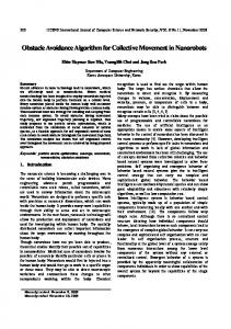
of some obstacle Ob is defined as the set of initial states for which the projections on the position space of all time-optimal trajectories intersect Ob. It is em to show that the extremal paths I’ and I’2 intersect d b from any state in the Dynamic obstacle Shadow [lo]. It follows that the time-optimal trajectory from an initial state, belonging to the dynamic obstacle sha&w, must coincide w!th some segment of the obstacle boundary, as shown in Figure 1. We call the return function for these states the constrained return function. Referring to Figure 1, the constrained trajectory, consists of three segments [lo]: 1) an unconstrained trajectory segment from the initial point, x, to the entry point, p1, on the obstacle boundary; 2) a constrained arc, which follows the obstacle boundary from
-
-=
0
\
segment 3
p2= p(s*.ij-
Segment 2
Figure 1: A Constrained Time-Optimal Path p 1 to the exit point, p 2 , and 3) an unconstrained trajectory segment from p2 to the target state, 0 . To derive the constrained return function, we need to determine the entry and exit points of the constrained arc and their corresponding speeds. To do so, we parameterize the obstacle boundary, h = (2,y), by the arc length, s:
h(s) = ( r s i n ( z ) r
+ u,rcos(z) + b) , s E [0,2m] (18) r
where ( U ,b) = c E R2 is the center of the obstacle, and r is its radius. Differentiating (18) with respect to time ields the velocity along a tra‘ectory that follows the oistacle boundary in terms 0) the tangent speed S: S
S
h(s) = (;.cos(-), -ssin(-)) r r The entry point, p 1 and the exit point pz, of the constrained arc, thus, correspond to the distances s 1 and s2, as shown in Figure 1, and their speeds correspond to B1 and sz, respectively. Using (18) and (19), it can be shown that the locus of all feasible states along the constrained arc in the state space of each joint describes an ellipse, which we call the velocity ellipse: 21-a
E2 2
) +(-) (7 -S
= 1
It follows that the entry and exit states of the constrained arc must belong to these two velocity ellipses in order for the trajectory to be dynamically feasible (twice differentiable) at p 1 and p2. The constrained return function is derived by com, any state puting the optimal motion time, ~ j from to the target state, which is the sum of the optimal motion times along Segments 1, 2 and 3, denoted TI, 72 and 73, respectively. To compute ~ f we , first determine the unknown entry and exit states,. S I , S I , s ~82,, using a parameter o timization that minimizes the total motion time wit[ res ect to these unknowns. The motion times a g n g the unconstrained segments, 71 and 73, are computed using (17): ~ ( x o , c , ~ , ~= I ,W ~ uI ()x o , p ( s 1 , 4 ) )
3077 -
(21)
where p ( s 1 , i l ) is the terminal state for Segment 1, as shown in Figure 1:
3.3
P(%4 S S S = (rsin(-) +a,scos(-),rcos(-)+b,-isin(-)) r r r r Similarly, r 3 is given by:
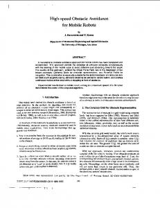
To consider multiple obstacles, we avoid an obstacle by using its individual return function. The trajectory is thus generated by switching from one return function t o another. The resulting pseudo return function is not a true return function since it is not guaranteed t o satisfy the HJB equation. It does, however, generate trajectories that are dynamically feasible, neartime optimal and terminate at the target. To illustrate the a proach, consider the two obstacles, Ob1 and Obz, sgown in Figure 2. Of the two extremal paths, I??) and I??), from the initial state X O , only I’y) intersects O b l . Hence, Ob1 can be avoided by computing the time-optimal path that is tangential to the obstacle at p(1l), as shown in Figure 2, using the unconstrained return function. Such a trajectory is uaranteed t o exist since the extremal trajectories en5ose the set of all feasible time-optimal trajectories [lo]. Therefore, we choose3 t o avoid Ob1 by using the unconstrained trajectory from the initial state t o pi‘). At pi1), both extremal paths, I??) and I??), intersect the second obstacle Ob2. Hence, Ob2 must be avoided using the constrained return function (27) until reaching the tangency point p f ) . From this point both I??) and I??) do not intersect any obstacle, permitting the use of the unconstrained return function (15) to the target. Henceforth, we denote p y ) the entry point and pp’the exit point of a trajectory segment slidin along obstacle k. Key to t f i s rocedure is the selection of the obstacle to be a v o i g d at a given state, which we call the nearest obstacle. To compute the nearest obstacle we first check if both extremal trajectories, obtained by integrating the extremal controls u?”(t) and u?”(t), intersect any obstacle, i.e., we determine the sets:
(22)
7 3 ( X f , c , r , sz, 9 2 ) = wu(P(s2,sz), X f ) (23) The computation of the optimal time along Segment 2, r2, is a s eczfied path time-optimal control problem, and can \e solved using the method presented in [9]. This approach obtains the time-optimal velocity profile in the s - S phase plane by maximizing the speed s while satisfying acceleration and velocity constraints due to the actuator limits and system drnamics. For simplicity, and with only a slight loss o optimality, we replace the true velocity limit, Smaz, which can be shown [lo] to lie between fi and l . l S f i , by its lower bound. Thus,
(24) We also avoid computing the time optimal velocity profile along the obstacle boundary by assuming a linear velocity profile between the terminal speeds along the constrained arc. Hence
Using (21), (23) and (as), we obtain the total motion time, r f ,from the initial state, X O , to the target state, xf, in terms of the unknown junction states:
+
~f(XO,Xf,C,r,Sl,sl,SZ,~z) = ~l(XO,C,~,~l,~l) 72(51, s i , sa, Sz)
+
,
7 3 ( x j C , T , S Z ,s 2 )
(26)
The constrained return function, wc, is, thus, obtained by minimizing 7-j over the parameters SI, S I , sa and 82 :
subject to (24) and the single obstacle constraint (4). Note that the cost function in (27) is a simple algebraic function, and that the minimization is carried out over only four parameters. Hence the computation of the constrained return function can be performed quickly usin an efficient gradient search. T i e computation of the constrained return function for one obstacle is not trivial although it is feasible for on-line computation given a few ”harmless” simplifications. However, the on-line computation of the return function for multiple obstacles would be virtually impossible due t o the large number of parameters. For the case of multiple obstacles, we, therefore, construct an a proximation of the return function, called the pseuio return function, which considers one obstacle at a time. This reduces the computationally complex Dynamic Problem with m obstacles to m computationally simpler problems. It is important to note that the assumption of convex obstacles only simplifies the computation of the constrained return function. General obstacles can be considered with additional computational cost [IO].
- 3078
The Pseudo Return Function for The Dynamic Problem
where dObi represents the boundary of Obi and p is the empty set. Defining the joint positions as p = (21, yl), we then determine those obstacles in I1 and I that are closest to the initial point, i.e., we compute t2e sets:
If there are more than one obstacles in Jdl and J d 2 , only the largest from each set is considered. The nearest obstacle, with index k, is that obstacle in Jdl and J d 2 which is closest to the initial point, PO. If Jdl 30ther unconstrained trajectories could also be used to avoid the
obstacle. However, this would be computationally
expensive
[lo]
more
The only points at which all obstacles are considered are the exit tangency points py), where the path switches from one obstacle shadow to another, since at those points the next nearest obstacle needs to be determined. The computational complexity at those points is, therefore, O(m). It should be noted that there may be specific cases, not discussed here, where Algorithm 1 may have to be modified (eg. recursive application by defining intermediate goals) [lo]. Figure 2: The Approximate Method and J d are not identical, then an unconstrained timeoptima? trajectory can be used to avoid the nearest obstacle. Otherwise all unconstrained time-optimal trajectories intersect the nearest obstacle, and the constrained return function (27) must be used to avoid it. If both J d l and J d 2 are empty any unconstrained trajectory can be used to drive the initial state to the tar'%t'illustrate the determination of the nearest obstacle, consider once again Figure 2. At the initial state x, J d l = {I}, J d 2 = (2) and the nearest obstacle is Obl. Therefore, the nearest obstacle Ob1 can be avoided using an unconstrained time-optimal trajectory tangential to the obstacle at ~(11). At p?), J d l = J d 2 = {2}, implying that the constrained return function must be used to avoid Obz. Finally, at py', J d l = Jd2 = { I } implying , any unconstrained timeoptimal trajectory can be used to reach the target. Thus, the pseudo return function, denoted cp, consists of the return function of the nearest obstacle at each state:
Extension to More General Manipulators and Obstacles The method presented here can be extended, as noted earlier, to manipulators with non-identity invariant inertia matrices using the coordinate transformation: 3.4
y=MB This converts (7) to the system: y=u
It also converts circular obstacles to elliptical obstacles. The solution ap roach remains unchan ed for the transformed system fecause elliptical obstaies can be parameterized simiIarly to (18). Generally shaped obstacles may be approximated by circles or ellipses in the manipulator joint space. General manipulators can be handled by using feedback linearization to convert the nonlinear dynamics to a second order linear system. The resulting nonlinear actuator constraints must then be conservatively approximated by constraints of the form (3). The method presented here could then be used for the online generation of dynamically feasible, obstacle-free trajectories satisfyin actuator constraints. The solution would, however,%e conservative and, hence, suboptimal ,
4
where w, and w, are given by (17) and (27) respectively. The avoidance procedure is outlined in the following algorithm: Algorithm 1: Step 1. Determine J d l , J d 2 . If both sets are empty, go to Step 4. Determine the nearest obz to Step 2. Otherwise, go stacle. If J d l # J ~ go to Step 3. Step 2. Avoid the nearest obstacle using an unconstrained trajectory tangential to the obstacle, as shown in Figure 2. Step 3. Follow the path generated by the constrained return function (27) until reaching the exit point p(2k). GO to step 1. Step 4. Use the unconstrained return function (17) to reach the target. STOP.
The paths generated by this algorithm are C2 con-
tinuous consisting of segments that are locally time-
o timaf. The computational effort at a typical oint afong the path is inde endent of the number of ogstacles since only one o&tacle is considered at a time.
(31)
Example The objective of this example is to avoid near-time optimally the three obstacles shown in Figure 3, starting at the initial state (0.0,0.0,4.0,-0.2) and terminating at the target state (O.O,O.O,O.O,O.O). Algorithm 1 resulted in the path shown in with motion time 4.7 seconds. Also shown Fi insigure 4 is a locally time-optimal path, computed using the method presented in [8], with motion time 4.4 seconds. The near-optimal ath correlates well with the locally optimal path. Further, the motion time of the near-o timalpath compares favorably with that of the globaiy optimal path, also shown in the Fi ure 4,which has a motion time of 4.25 seconds. %he difference between the near-time optimal ath, generated using the seudo-return function, a n i the lobally optimal. p a t i can be explained by the fact k a t for this initial state, there are two time-optimal paths (with the same motion time), avoiding the first obstacle, Obl, that lie on either side of Obl. Numerical approximations in the minimization (27) resulted in the path to the ri ht of the obstacle being selected. However, selecting d e path to the.left of the obstacle would have resulted in a near-optimal path closer to the globally optimal path.
",g,
3079 -
Initial Point
Initial Point
\f
\
Exit Point
Globally Optimal Path
Target Figure 3: Near-Time Optimal Path for the Example
5
Locally Optimal
Figure 4: Time-Optimal Paths for the Example
_141_
Conclusions
A method for the on-line generation of obstaclefree, dynamically feasible, and near-time optimal trajectories for robotic manipulators with invariant inertia matrices has been presented. The near-optimal paths are generated by minimizin5the time-derivative of the pseudo-return function, w ich is an approximation of the return function for this roblem, and is computed by considering one obstacye at a time. This reduces the computational effort significantly b reducing the complex problem of time-optimal avoidI ance of m obstacles to m simpler problems, each consisting of the time-optimal avoidance of one obstacle. The trajectories generated b the pseudo return function are near-optimal since tKey are com osed of se ments which are each locally optimal. ‘$he exam presented in the paper demonstrates a close correyation between the near-o timal and optimal paths. The computation of t%e pseudo return function degends on only one obstacle at all but a finite numer of tan ency points, where the tra’ectory switches from the g n a m i c obstacle shadow obstacle to another. he proposed approach is, therefore, applicable to the on-line computation of near-time optimal trajectories of a class of robotic manipulators, or mobile robots, moving in environments containing a large number of obstacles.
alone
Target
M.E. Khan and B. Roth, ”The near-minimum time control of open loop articulated kinematic chains”, Journal of Dynamic Systems Measurements and Control, Volume 93, Number 3, pp. 164-172, Sept. 1971.
[5] E.B. Meier and A.E. Bryson, ”An efficient algorithm for time-optimal control of a two-link manipulator”,
Proceedings of the AIAA Conference on Guidance and Control, Monterey, CA, pp. 204-212, 1987. [6] A.I. Moskalenko, ”Bellman Equations for Optimal Pro-
cesses with Constraints on the Phase Coordinates”, Automation and Remote Control, 4:185 3-1864, 1967.
[7] N.E. Nahi, ”On the Design of Time-Optimal Systems via the Second Method of Lyapunov”, IEEE Trans. Automatic Control, pp. 274-276, 1964. [8] Z. Shiller and S. Dubowsky, ”Time-optimal path-
planning for robotic manipulators with obstacles, actuator, gripper and payload constraints”, International Journal of Robottcs Research, pp. 3-18, Dec. 1989. [9] Z. Shiller and H.H. Lu, ”Computation of time-optimal motions along specified paths”, ASME Journal of Dynamic Systems Measurements and Control, December 1991.
References
[lo]
M. Athans, Optimal Control, Academic Press, New York and London, 1965.
J.E. Bobrow, S. Dubowsky and J.S. Gibson”, ”TimeOptimal Control of Robotic Manipulators”, International Journal of Robotics Research, Volume 4, Number 3, 1985. [31 L.
-
Cesari, Optimization Theory and Applications: Problems with Ordinary Diflerential Equations, Springer-Verlag, New York, 1983.
-3080-
S. Sundar, Near-Time Optimal Feedback Control of Robotic Manrpulators, Ph.D. Dissertation, Dept. of
Mechanical Engineering, University of California, Los Angeles, CA, 1995. [ll] S. Sundar and Z. Shiller, ”Optimal Obstacle Avoidance Based on the Hamilton-Jacobi-Bellman Equation”, Proceedings of the 1994 IEEE International Conference on Robotics and Automation, San Diego.