IJCSNS International Journal of Computer Science and Network Security, VOL.6 No.10, October 2006
1
Time Series Data Mining for Multimodal Bio-Signal Data Masaki Aono, Yuske Sekiguchi, Yoshifumi Yasuda, Naoya Suzuki, and Yohei Seki,
[email protected] Toyohashi University of Technology, 1-1 Tempakucho, Hibarigaoka, Toyohashi, Aichi, JAPAN Summary It is believed that there is a close correlation between the physical and mental activities of human body. These physical activities can be measured using various multimodal bio-signals employing either invasive or non-invasive sensors. In contrast, although mental activities have been modeled from various standpoints, they have been associated mostly with brain activities. We have focused on mapping physical multimodal bio-signals as time series data with mental states such as somnolence, fatigue, and concentration. We will discuss two mathematical data mining tools: (1) the interval cross-correlation coefficient; and (2) the interval crosscovariance function coefficient. Given a multimodal time series bio-signal data acquired at a given frequency using non-invasive sensors attached to a human volunteer, our methods aimed to predict the mental state of a human subject. The primary objective was to examine the feasibility of our methods in predicting the mental state of students during lessons in a university classroom. Previous attempts to predict mental states from bio-signals have mostly been based on electroencephalogram (EEG), electrocardiogram (ECG), or electrooculogram (EOG), but have not tried to combine them. However, it is often difficult to obtain stable EEG signals from students in a university classroom because of artifacts arising from body and eye movements. Based on this observation, we considered simultaneous multimodal bio-signals with their combination, and introduced interval cross- correlation coefficient and interval cross-covariance function coefficient as data mining tools for mapping the physical and mental states of the human body. We conducted experiments using subjects equipped with multiple sensors, and compared the results with the outputs of our data mining methods. Preliminary experiments show that our method produces reasonable results and allows us to control the experimental parameters to cope with individual variations. Our method is also applicable to monitoring personal health care, vehicle drivers, and individuals in business group meetings.
Key words: time-series data analysis, multimodality, prediction, biosignals
Introduction Mining latent correlations from multimodal, streaming, time series bio-signal data is a relatively new field of research in science and engineering that includes many inherent multidisciplinary technical challenges. The first challenge is how to achieve a quick response, since bio-signal data are usually
Manuscript received September 28, 2006. .
measured in real time, sometimes from many different sources (i.e., multimodality), obtained using a variety of sensor devices. The second challenge is how to remove noise and outlying data that could mislead the mining algorithms, and this requires an algorithm to be robust and accurate. This is a prerequisite, because noninvasive-type sensors are usually very sensitive to human movements, even if the subject moves only slightly during sensor monitoring. The third challenge is to align the different sources of bio-signal data, whose frequencies may differ from source to source, and whose data could be missing from time to time. The fourth challenge is how to acquire and manage the bio-signal data from a group of subjects equipped with sensor devices simultaneously and asynchronously. The fifth challenge, which is the most difficult, is to map a given mental state (such as “state of concentration”, “state of fatigue”, and “state of somnolence”) to one or more of the physical biosignals. Based on observations obtained from off-line measured time series bio-signal data, we will discuss the use of two algorithms to cope with some of the above challenges, and to attempt to lay the foundation for future study in this area of research. It should be borne in mind that there is not an established method of handling all the challenges mentioned above. In the following, we will briefly survey related work in Section 2. In Section 3, we will review and introduce mathematical tools that we used for mining the time series biosignal data. In Section 4, we describe our observations based on off-line measured bio-signal data, followed by our predictions of the state of concentration and the state of somnolence in Section 5. A prototype smart classroom system, HIBALIS, is briefly described in Section 6, and our conclusions are given in Section 7, along with a discussion of our approach and possible future research.
2. Related Work Time series data analysis has a long history. Given the data for a time series, Auto-Regressive Moving Average (ARMA) models have been used extensively to predict what could happen next in meteorology, astronomy, geology, economy, and many other academic fields [1, 2]. Recently, emerging technologies and algorithms using time series data mining have been published in the fields of computer science and engineering, for example, in collecting time series data, and defining the similarities, clustering, and classification [3, 4, 5]. Lin et al. [6] classified time series data mining into three large tasks: (1) subsequence matching; (2) anomaly detection; and (3) time series motif
IJCSNS International Journal of Computer Science and Network Security, VOL.6 No.10, October 2006
2
discovery. They also mentioned visualization aspects of time series data. However, there have been few approaches that have tried to understand the correlation between two or more time series (i.e., multimodal time series) obtained simultaneously. One example is described in a paper by Gruhl et al. [7] that addresses the correlation between reputation (as one time series data) written in as a Weblog (blog) on newly published books, and their sales trends (the other time series data) published on the Amazon.com website. They showed that there was a close correlation between the two time series. Once the reputation of a newly published book became established, its volume (as time series data) in the blog thread exhibited a sharp peak at a given time, and then, after a slight time delay, the book’s sales tended to increase. The corresponding sales rank (as time series data) tended to be depicted as a sharp peak a few days after the blog thread. Crone et al. [8] employed neural network predictions for inventory decisions. The basic idea was to forecast a one-step future data point using n preceding points. They stated that their method was analogous to that used in Auto-Regressive models.
3. Interval Cross-correlation and Crosscovariance Here, we assume that time series data are acquired as a set of (sampled) numerical data, and review the mathematical tools for analyzing multimodal, multivariate time series data: the sample cross covariance and sample cross correlation methods. Then we introduce the “interval cross-correlation coefficient” and “interval crosscovariance function”.
values in the range [−( n − 1), n − 1] . The value of k corresponds to a discrete (sampled) time. For a given positive value of k , if the absolute value of rxy ( k ) is relatively large (e.g., >0.5), then the time series data denoted by x has some correlation with another time series data denoted by y . Suppose that we have M different multimodal time series data, then the above equation represents a correlation matrix of size M × M , which makes it possible to perform multivariate analysis.
3.2 Interval Cross-correlation Coefficient The value of rxy ( k ) not only depends on k , but also depends on n . If n is very large (e.g., 100,000), interactive analysis is less likely. Thus, we considered subdividing the entire set of sample data into smaller “intervals” of equal size m , as shown in Fig. 1. The problem of cross correlation among the multimodal biosignal time series data was then reduced to the same problem but with smaller sample sizes. For simplicity, in the ensuing discussion we assume that n = pm , where n is the total number of given time series data, p is the number of intervals, and m is the number of samples in each interval. n samples time series data
m sampled times series data
m sampled times series data
m sampled times series data
p intervals
Fig. 1 Time series bio-signal data can be subdivided into
p intervals of
3.1 Sample Cross-Correlation
m samples.
Suppose two sets of n time series data x = x1 , ..., xn and y = y1 , ..., yn are given. Then, sample cross-covariance is given as follows:
Consider an arbitrary interval, j ∈ [1, .., p ] , and a pair of j j sample time series data sub-sequence x ( j ) = x1 , ..., xm j j and y ( j ) = y1 , ..., ym . We define interval cross-correlation coefficient as shown in Equation (1).
⎧ 1 n− k ⎪ ⎪ ∑ ( x − μ(x))( yt +k − μ(y )) k = 0,..., n −1 ⎪ ⎪ n t =1 t , cxy ( k ) = ⎪ ⎨ n ⎪ 1 ⎪ ⎪ ∑ ( xt − μ(x))( yt +k − μ(y )) k = −1,..., −n + 1 ⎪ ⎪ ⎩ n t =1−k where μ ( x ) represents the mean of x = x1 , ..., xn , and μ ( y ) represents the mean of y = y1 , ..., yn . Then, sample cross- correlation coefficient is given as follows:
rxy (k ) =
cxy ( k ) cxx (0)c yy (0)
The value of rxy ( k ) in the above equation ranges from –1 to +1, and it varies with the integer k , which assumes
j
rxy ( k ) =
c xy ( k )
j
j
(1)
j
cxx (0)c yy (0)
Equation (1) represents an M by M correlation matrix, assuming that we have M multimodal bio-signals, as depicted in Table 2 in Section 5.1.
3.3 Interval Cross-covariance Function Here we introduce a mathematical tool which is similar to the “interval cross correlation” in that we are interested in a characteristic value in a specific “interval” (i.e., the local mental activity). Unlike measuring the correlation
IJCSNS International Journal of Computer Science and Network Security, VOL.6 No.10, October 2006
between two bio-signal data per se, we define the j-th interval cross-covariance function as follows: F ( f x , g y , j ; Δt ) ≡ j
∫
t +Δt
t
j
( f x (t ) − f x ) dt j
∫
t
t +Δt
j
( g y (t ) − g y ) dt , (2) j
j
where f x (t ) and g y (t ) represent functions of specific biosignals at the j-th interval, and Δt represents the length of the j j interval. It should be noted that f x (t ) and g y (t ) may be functions of the same bio-signal. We then define j-th interval cross-covariance function coefficient as: F ( f x , g y , j ; Δt ) . (3) ρ ( f x , g y , j ; Δt ) = F ( f x , g x , j ; Δt ) F ( f y , g y , j ; Δt ) This coefficient is similar to the ordinary cross coefficient of two statistical variables, x and y, except that two functions are used instead of two variables (or bio-signals per se). For example, the interval cross-covariance function coefficient of EOG and EEG using low pass filters as their functions can be used to predict a complete period of sleep (i.e., non-REM sleep). However, we would expect that this value could also be used to predict the degree of somnolence, or the beginning of the state of somnolence.
3
measured at 200 Hz, Fig. 2(b) shows the one-tenth downsampled data, and Fig. 2(c) shows the one-twentieth down-sampled data. It is clear that one-twentieth downsampling could lose any macroscopic behavior, while onetenth down-sampling was able to keep the overall global behavior. From this experiment, we decided that the down-sampling rate would be one-tenth the original raw data rate. It should be noted that the original data may include noise and spikes. Thus, during the down-sampling process, we performed averaging using the standard Exponential Moving Average (EMA) technique [9] shown in Equation (3). (4) ema[i ] = w × data[i ] + (1 − w) × ema[i − 1] , where ema[i ] denotes the EMA value at time i , data[i ] denotes the raw data at time i , and w denotes the parameter weight. As w approaches the value of 1.0, it begins to reflect the raw data more, while as w approaches the value of 0.0, it begins to reflect the previous EMA value more.
3.4 Down-sampling and Removal of Noise The interval subdivision technique described in the previous section enabled us to reduce the computation time for cross correlation between two time series biosignal data subsequences. However, in ideal conditions, the feasible online monitoring period of human sensor data is, at most, between 10 and 30 seconds for monitors (e.g., teachers) to provide feedback to the subjects (e.g., students). For example, to compute the cross correlation between two time series over a period of one minute is only possible after the lapse of another additional minute. Considering the above, the period for reporting analysis results is at least 30 seconds. Therefore, we assumed the interval period was approximately 30 seconds (at most), and computed the cross correlation between two different time series bio-signal data subsequences. The sampling rate of the sensor devices was 100 to 200 Hz, which depended on the particular sensor device used and the biosignal that we chose to measure. Thus, the volume of time series bio-signal data obtained within a period of 30 seconds was 3,000 to 6,000 samples. Using Equation (1) to compute the cross correlation required us to compute the correlation between the current and the previous 30 seconds data, as well as the correlation between the current and the next 20 seconds data, which amounted to 6,000 to 12,000 computations. This was prohibitively large. Then we conducted down-sampling of the original data, such that the macroscopic behavior of each biosignal data was not lost. Fig. 2 shows EEG data of a subject during the first 10 seconds of sampling. Fig. 2(a) shows the raw data
(a)
(b)
(c) Fig. 2 EEG profiles of a subject in the first 10 seconds: (a) original raw data, (b) 1/10-th down-sampled data, and (c) 1/20-th down-sampled data.
4. Observation from Off-line Measurement of Multimodal Bio-signal Data We conducted off-line recording and measurement of human bio-signal data from several subjects based on a specific agenda, as shown in Table 1, including relaxation, concentration (such as performing simple calculations and listening to English), and time spent watching videos, which lasted approximately one hour in total.
IJCSNS International Journal of Computer Science and Network Security, VOL.6 No.10, October 2006
4
Table 1 Experimental agenda of the subjects.
Start Time (minute) 0 3 7 12 18 22
Duration (minute(s)) 3 4 5 6 4 42
Contents Rest (relaxed) Calculation (addition) Rest and recovery Silent English translation Rest and recovery Video watching
Fig. 3 shows the eight different multimodal bio-signals measured: EEG, α, β, δ, and θ waves, EOG, breathing (respiratory oscillation), and pulse waves (PW). The α, β, δ, and θ waves were calculated from the EEG data. As shown in the ellipses contained in Fig. 3, during intellectual activity, the δ wave signal decreased, while the breathing (respiratory oscillation) signal tended to have a relatively low amplitude, but be very regular. In contrast, during the relaxed state, both the δ wave and the breathing signals (respiratory oscillation) tended to be irregular, but their amplitudes increased compared to the state of intellectual activity. Note also that during intellectual activity, the EOG trace was intermittent, relatively regular, and positive values were dominant, but during the relaxed state, the EOG trace was relatively large and irregular, and both positive and negative values were observed.
combinations of two out of eight multimodal bio-signals, we chose the δ wave and breathing (respiratory oscillation) signals, as discussed in the previous section.
5.1 Predicting the State of Concentration Using Interval Cross-Correlation Coefficient In this section, we will describe a method for predicting the state of concentration using the interval crosscorrelation coefficient. The basic idea is as follows. If, for a given period, (within 30 seconds as described in Section 3.4) with a one-tenth down-sampling of the time series, the absolute value of (or square magnitude of) the i-th i interval cross correlation rxy ( k ) between two bio-signals is significantly larger than the j-th interval cross j correlation rxy ( k ) between the same two bio-signals, where i ≠ j , then this can be utilized to predict mental activity. Among all the possible combinations of the eight biosignals shown in Table 2, we chose the δ wave and breathing (respiratory oscillation, ‘BR’ in Table 2) signal. Table 2 shows the “significance matrix”, where a “++” entry denotes a significant difference between the two biosignals during concentration and relaxation states, a “+” entry indicates the possible difference between the two bio-signals, while a “-” entry indicates no difference between the two bio-signals. The data in Table 2 was created by selecting three different pairs of intervals, each having a state where a subject was concentrating on something, and also having the state where a subject was relaxed. We then average these values, and found that either a (δ, BR) or a (BR, PW) pair showed a significant difference in their cross-correlation coefficients among all the combinations, where PW denotes a Pulse Wave. The (δ, θ) pair can also be used. We chose the (δ, BR) pair for our experiments to predict the state of concentration, since this pair exhibited a more significant difference than the (BR, PW) pair did. It is very interesting that this result coincides with the observations described in Section 3.4. Table 2 Significance matrix of interval cross-correlation coefficients, contrasting the state of concentration with the state of relaxation.
EEG δ θ
Fig. 3 Eight different multimodal bio-signals measured from a subject during the first 10 minutes.
α
EEG
δ
θ
α
β
EOG
BR
PW
N/A
-
-
-
-
-
-
-
+
-
-
-
++
-
N/A
-
-
-
-
-
-
-
-
-
N/A
-
-
-
N/A
N/A
β EOG
5. Predicting Mental States
N/A
BR PW
Based on the observations discussed in the previous section, we developed an algorithm to predict the mental state of several subjects from their multimodal bio-signals. Among the many
-
-
N/A
++ N/A
j
Fig. 4(a) shows the two rxy ( k ) curves between the δ wave and breathing (respiratory oscillation) signals, j where the solid curve represents rxy ( k ) for the state of
IJCSNS International Journal of Computer Science and Network Security, VOL.6 No.10, October 2006
relaxation starting from 20 minutes and ending at 20 minutes and 30 seconds, while the dotted curve represents j rxy ( k ) for the state of concentration starting from 5 minutes and ending at 5 minutes and 30 seconds. Note that using a one-tenth down-sampling rate in the data measured at 200 Hz, the number of samples (i.e., m in Fig. 1) was 600. In Fig. 4(a), it is still rather difficult to see any difference between the two different states. Thus, we j defined the “square magnitude” of rxy ( k ) , as shown in Fig. 4(b). Using this measure, it is easier to see that the two different states exhibit different “square magnitude” values in their “interval cross correlation” analysis.
5
Fig. 4 shows a typical contrast between the state of concentration and the state of relaxation. This particular example used a time-sliced window of 30 seconds, and identified performing “mental arithmetic” as a typical example of an intellectual activity. Other choices, such as “Silent reading of English”, could also be detected, as listed in Table 1, which exhibited more or less similar behavior and exhibited similar graphical behavior. Based on these behaviors, we tentatively defined the state of concentration using the following formula:
∫
t
t +Δt
(| rδ , b (t ) | −η ) dt < λ , 2
j
(5)
j
where rδ , b (t ) denotes the j-th interval cross correlation
(a)
between the δ wave and the breathing (respiratory oscillation) signals, and η and λ are nonnegative constants. If the left-hand side of the inequality in Equation (5) is denoted by R ( x, y , j , η ; Δt ) , then the state of concentration can be predicted if R ( x, y , j , η ; Δt ) is less than a pre-defined threshold, λ . Otherwise, we predict that the subject is in the state of relaxation. Formally, the “concentration detector” algorithm is given below: Algorithm Concentration-detector Let Δt be the actual interval (e.g. 30 seconds) Let Let Let
j
rx , y (t ) be defined as in Equation (1)
x be the δ wave y be the breathing signal (BR in Table 1)
Initialize jSave as zero For t in timesteps do
(b)
j = ⎢⎣ t / Δt ⎥⎦ R = 0.0 if ( j == jSave ) then R += | rx , y (t ) | −η j
2
else do jSave = j if ( R < λ ) then Mark the (j-1)-th interval as “Concentrated” else Mark the (j-1)-th interval as “Relaxed” end do endif
(c) Fig. 4 (a) A plot of the interval cross-correlation coefficient of the δ waves and breathing (respiratory oscillation) signals for two different intervals, where the solid curve denotes the relaxed state, and the dotted curve denotes the state of concentration while performing mental arithmetic (i.e., addition). (b) and (c) show the “square magnitude” of these interval cross-correlation coefficients, respectively.
Fixing Δt and λ to predefined constants, and varying η between 0.0 and 0.1, we applied the above algorithm to two subjects. By utilizing a standard confusion matrix [10], which counted as True Positive (TP, predicted as a concentration that was a real subject concentrating), False Positive (FP), True Negative (TN, predicted as being relaxed, which was a real subject who was relaxed), or False Negative (FN), we obtained the resulting ROC curve
IJCSNS International Journal of Computer Science and Network Security, VOL.6 No.10, October 2006
6
shown in Fig. 5. The correct answers were confirmed using both video observations (as shown in Fig. 6) and the answers to mental arithmetic problems (addition) from each subject. From the data in Fig. 5, it is interesting to note that Subject 2 exhibited an ideal ROC curve, while Subject 1 showed a plateau before reaching a TPR = 1.0. Since the ROC curve of a good classification model should be located as close as possible to the upper left corner of the diagram, our simple concentration detector algorithm was reasonably accurate for the given time series bio-signal data. The individual variations, especially visible in the ROC curve of Subject 1, can be interpreted as showing that several intervals corresponding to concentration and relaxation are intermediate states between concentration and relaxation
Fig. 5: The concentration detector ROC curves of two subjects calculated by varying η in Equation (5) between the values of 0.0 and 1.0.
5.2 Predicting the State of Somnolence Using Interval Cross-Covariance Function In this section, we will describe a simple method for predicting the state of somnolence. Note that here we are interested in the onset or the degree of somnolence, and also in complete somnolence, which should be easier to detect (e.g., by video observation, as shown in Fig. 8(b)). The detection of the state of somnolence has been more extensively studied in many fields of science and engineering. For example, Fukami et al. [11] used an Auto-Regressive (AR) model, with α , δ , and θ data to extract the characteristic patterns during sleep, and achieved a >80% success rate. Kameyama and Doi [12] employed a portable sensor to measure pulse waves obtained from the fingertips of subjects in order to extract fluctuations in the heartbeat rate. They attained a 75% success rate in identifying “shallow” and “deep” sleep. Telser et al. [13] described sleep stage transitions based on monitoring the heart rate variability (HRV), and succeeded in differentiating between REM sleep and NREM sleep to some extent. We had the simple idea of constructing a “somnolence detector” in employing the square magnitude of the interval cross correlation, similar to the process used in the “concentration detector” discussed earlier. However, as shown in Table 3, we examined every combination between the two bio-signals under three different conditions with different subjects at different time intervals, and found that there was no good detector that was positive (“+”) for all the three conditions. Table 3: The significance matrix of the square magnitude of the interval cross-correlation coefficient, contrasting the state of somnolence with the state of arousal. Three different pairs of intervals were examined, but it turned out that no combination could satisfy all three conditions. (Note: EEG column is omitted.)
(a)
(b)
δ
θ
α
β
EOG
BR
PW
EEG
+,-,-
-,-,-
-,-,-
-,-,-
-,+,-
-,+,-
+,-,-
δ
N/A
-,-,-
-,-,-
-,-,-
-,-,-
-,-,-
-,-,-
-,-,-
+,+,-
+,-,-
+,-,-
-,-,-
N/A
-,-,-
-,-,-
-,-,-
-,-,+
N/A
-,-,-
-,-,-
-,-,-
N/A
-,-,+
-,-,-
N/A
+,+,-
θ α β EOG BR PW
(c)
(d)
Fig. 6 Subject 1 in (a) a state of concentration and (b) a state of relaxation, and Subject 2 in (c) a state of concentration and (d) a state of relaxation.
N/A
N/A
Thus, we attempted to resolve this problem from a different standpoint. The data in Fig. 3 shows that the EOG values tend to be predominantly positive if the subject is in the state of concentration (e.g., staring at a monitor), whereas the EOG values tend to fluctuate between both positive and negative values when the subject is in the relaxed state. This phenomenon seems to
IJCSNS International Journal of Computer Science and Network Security, VOL.6 No.10, October 2006
be more clearly followed in the state of somnolence, although the magnitude of the EOG values tends to decrease. Thus, we attempted to predict the sign of somnolence by applying the EOG values to Equation (2), as below: H≡∫
t + Δt
(| G | −| G
t
|) dt ∫
t + Δt
(G − G ) dt ,
7
obtained a set of human-determined correct answers (i.e., either being awake or not) for each interval. Then we ran our method using Equation (6) by varying τ , and obtained the results shown in Fig. 7.
(6)
t
where G (t , j ,τ , κ ) = Function (EOG
j
(t ), τ , κ )
Function ( x , τ , κ ) = LPF ( x , τ ) + Amplify ( x; | x |> κ ) .
LPF ( x , τ ) is a low-pass filter, and τ is a control parameter. Amplify ( x; | x |> κ ) is an amplifier for the bio-signal data,
x , whose absolute value exceeds the threshold, κ . By applying Equation (6) to Equation (3), we can obtain the main component of somnolence detector as ρ (| G ( x ) |, G ( x ), j , τ , κ ; Δt ) . By analogy with Equation (5), we can formally define the somnolence detector as follows: (7) ( ρ (| G ( x ) |, G ( x ), j , τ , κ; Δt ) − ζ ) < μ If the left-hand side of Equation (7) is denoted by Q ( x , y , j , τ , κ , ζ ; Δt ) , then the state of somnolence can be predicted if Q ( x , y , j , τ , κ , ζ ; Δt ) is less than a predefined threshold, μ . Otherwise, we predict that the subject is in the state of arousal. Formally, “somnolence” detection algorithm is as below: 2
Algorithm Somnolence-detector Let Δt be the actual interval (e.g. 30 seconds)
Let
ρ ( f ( x ), g ( y ), j ; Δt ) be defined as in Equation (3) x and y be EOG f ( x ) be a smoother (low pass filter and amplification)
Let
g ( x ) be the absolute of f ( x )
Let Let
Initialize jSave as zero For t in timesteps do
j = ⎢⎣t / Δt ⎥⎦ Q = 0.0 if ( j == jSave ) then Q +=
ρ (| G ( x ) |, G ( x ), j ; Δt )
2
Fig. 7: The ROC curve of the somnolence detector calculated by varying τ and κ in Equation (6)
Fig. 8 shows the data obtained on Subject 1 while watching the TV program and moving between the state of arousal and the state of somnolence. Specifically, the horizontal axis denotes the time from the start of the TV program, and the vertical axis represents the “arousal level” (the inverse of the somnolence level) corresponding to the value of ρ (| G ( x ) |, G ( x ), j , τ , κ ; Δt ) . The dotted curve shown in Fig. 8 shows the change in actual arousal level, while the solid curve was calculated using the somnolence detector algorithm. The correct answer was calculated by manually examining the subject’s face from a video clip and was identified frame by frame. Fig. 9(a) and 9(b) show snapshots obtained while the subject watched the TV program. In Fig. 9(a), Subject 1 was in the state of arousal, while in Fig. 9(b), Subject 1 was in the state of somnolence. Similarly, Fig. 9(c) and 9(d) show Subject 2 is in the state of arousal and in the state of somnolence, respectively
−ζ
else do jSave = j if ( Q < μ ) then Mark the (j-1)-th interval as “Somnolent” else Mark the (j-1)-th interval as “Awake” end do endif
We conducted an experiment for identifying the state of somnolence or the state of arousal by taking the video of a subject while he was watching a TV program “Natural beauty of Japan” lasting approximately 30 minutes By selecting the interval to be 30 seconds, as discussed in Section 3, and by identifying the subject’s facial expression to see if they were awake or somnolent, we
Fig. 8: The accuracy of our somnolence detector calculated by comparing the actual state of somnolence of Subject 1. The dotted curve is the actual arousal level, while the solid curve was calculated using the somnolence detector algorithm. The correct answer (dotted curve) was measured by manually examining records of the subject’s face (in mpeg format), and was identified frame by frame.
IJCSNS International Journal of Computer Science and Network Security, VOL.6 No.10, October 2006
8
Fig. 10 Components and data flow of HIBALIS, a smart classroom. Fig. 10 shows a diagram of the HIBALIS components, and Fig. 11 shows a demonstration lecture having five students (subjects) each sitting on a “smart chair” that is capable of sensing eight bio-signals simultaneously, including three EEGs, two EOGs, an ECG, and a breathing signal. The mining of groups of bio-signals is currently underway.
(a)
(b)
Fig. 11 Lecture demonstration of HIBALIS, involving a smart classroom using five students as subjects sitting on smart chairs.
(c)
(d)
Fig. 9 Subjects watching the TV program “The natural beauty of Japan”. Subject 1 in (a) a state of arousal and (b) a state of somnolence; Subject 2 in (c) a state of arousal and (d) a state of somnolence.
6
HIBALIS: Smart Classroom as an Application of Data Mining
Toyohashi University of Technology (TUT) in Japan, has carried out an “Intelligent Human Sensing” project for several years as a 21st Century Center of Excellence (COE) project sponsored by the Japanese government. In this project, we are implementing a smart classroom called HIBALIS, where a lecturer and students can interact with each other, while the lecturer can monitor the mental state as well as observe physical bio-signals from sensor devices attached to each student in real time.
7
Conclusions
Given multimodal time series bio-signal data obtained from a variety of sensor devices, we developed two algorithms and associated data mining tools, i.e., the square magnitude of the interval cross-correlation coefficient and the square magnitude of the interval crosscovariance function coefficient, to estimate the mental state of subjects, such as the state of concentration and the state of somnolence. The advantage of our method is that it is simple and straightforward, and it allows us to perform real-time decisions as to whether a subject is in the state of concentration or whether they are in a state of somnolence, by monitoring at intervals and by applying our data mining methods to each interval. In the experiments we conducted, we took the interval to be 30 seconds, which implies that we can obtain an answer every 30 seconds by continuously monitoring a subject’s bio-signals. The disadvantage of our method is that both the interval crosscorrelation coefficient and the interval cross-covariance function coefficient are susceptible to artifacts caused by quick movements by the subject, such as twitches and jerks. However, as far as our experiments go, the ROC curves of both our concentration detector and our somnolence detector showed a good performance level.
IJCSNS International Journal of Computer Science and Network Security, VOL.6 No.10, October 2006
In the future, we would like to begin analyzing the biosignals of a group of subjects, and extend our method to analyzing the data from this group of subjects.
Acnowledgements This work was supported by the 21st Century Center of Excellence (COE) program of the Japanese government. We are also grateful to numerous staff and students in the COE project.
References [1] Hamilton, J. D. Time Series Data Analysis, Princeton University Press, 1994. [2] Chatfield, C., The Analysis of Time Series -An Introduction, Sixth Edition, CRC Press Company, Boca Raton, Florida, 2004. [3] Chiu, B., Keogh, E. and Lonardi, S. Probabilistic Discovery of Time Series Motifs, Proceedings of the Ninth ACM SIGKDD International Conference on Knowledge Discovery and Data Mining, ACM Press, Washington, D.C. 2003, pp.493-498. [4] Vlachos, M., Hadjieleftheriou, M., Gunopulos, D. and Keogh, E. Indexing Multi-Dimensional Time-Series with Support for Multiple Distance Measures, Proceedings of the Ninth ACM SIGKDD International Conference on Knowledge Discovery and Data Mining, ACM Press, Washington, D.C. 2003, pp.216-225. [5] Keogh, E. and Ratanamahatana, C. A. Exact Indexing of Dynamic Time Warping, Knowledge and Information Systems, Vol. 7, 2004, pp. 358-386. [6] Lin, J., Keogh, E., Lonardi, S., Lankford, J. P., and Nystrom, D. M. Visually Mining and Monitoring Massive Time Series, Proceedings of the Tenth ACM SIGKDD International Conference on Knowledge Discovery and Data Mining, ACM Press, Seattle, WA, 2004, pp.460-469. [7] Gruhl, D., Guha, R., Kumar, R., Novak, J. and Tomkins, A. The Predictive Power of Online Chatter, Proceedings of the Eleventh ACM SIGKDD International Conference on Knowledge Discovery and Data Mining, ACM Press, Chicago, IL, 2005, pp.78-87. [8] Crone, S. F., Lessmann, S., and Stahlbock, R. Utility based Data Mining for Time Series Analysis – Cost-sensitive Learning for Neural Network Predictors, Proceedings of the 1st international workshop on Utility-based data mining UBDM, Chicago, 2005, pp.59-68. [9] Pyle, D. Data Preparation for Data Mining, Morgan Kaufmann, San Francisco, 1999. [10] Tan, P-N., Steinbach, M. and Kumar, V. Introduction to Data Mining, Addison-Wesley, Boston, 2006. [11] Fukami, T., Emori, R., Shimada, T., Akatsuka, T., and Saito, Y. The Detection of EEG Characteristic Waves by Using Locally Stationary Autoregressive Models, Trans. IEE Japan, Vol. 121-C, No.3, in Japanese 2001 , pp.1-7. [12] Kameyama, K. and Doi, M. IT Technology Trend Supporting Health Life, Information Processing, Vol. 46,
9
No.10, Information Processing Society of Japan, in Japanese 2005, pp. 1144-1154. [13] Telser, S., Staudacher, M., Ploner, Y., Amann, A., and Hinterhuber, H, and Ritsch-Marte, M. Can One Detect Sleep Stage Transitions for On-Line Sleep Scoring by Monitoring the Heart Rate Variability? Somnologie, Vol. 8, 2004, pp.33-41. Masaki Aono received the B.S. and M.S. degrees in Information Sciences from the University of Tokyo in 1980 and 1984, respectively. He received his Ph.D. degree at computer science department of Rensselaer Polytechnic Institute in 1994. During 19842003, he worked with Tokyo Research laboratory, IBM Japan Ltd. Since 2003. he is a professor at computer and information sciences in Toyohashi University of Technology. His research interests include data mining, information retrieval, multimedia data processing, and information visualization. Yuske Sekiguchi received the B.S., M.S. and Ph.D. degrees from Tokyo Institute of Technology in 1996, 1998 and 2003, respectively. He is currently postdoctoral fellow at Research Center of Physical Fitness, Sports and Health, Toyohashi University of Technology. His research interests include drowsy state of human and sleep of dolphin.
Yoshifumi Yasuda received his B.S.degree from Tokyo University of Education. He also received the Ph.D. degree in physiology from Nagoya City University Medical School, Japan, in 1992. He is now a professor in the Health Science Center in Toyohashi University of Technology. His current research interest is the use of thoracic impedance and an ultrasonograph for assessing cardiorespiratory function in humans. Naoya Suzuki received his B.E. from the department of Production Systems Engineering, Toyohashi University of Technology in 2006. He is currently a student of the Graduate School of Engineering, Toyohashi University of Technology. Yohei Seki received the B.S. and M.S. degrees in Computer Sciences from Keio University in 1994 and 1996, respectively. He received his Ph.D degree at department of informatics in the Graduate University for Advanced Studies in 2005. During 2002, he worked as a research associate in
10
IJCSNS International Journal of Computer Science and Network Security, VOL.6 No.10, October 2006
Aoyama Gakuin University. Since 2005. he is a research associate at computer and information sciences in Toyohashi University of Technology. His research interests include natural language processing, summarization, opinion analysis, and text generation.