Time-Series Modeling for Statistical Process Control Author(s): Layth C. Alwan and Harry V. Roberts Source: Journal of Business & Economic Statistics, Vol. 6, No. 1 (Jan., 1988), pp. 87-95 Published by: Taylor & Francis, Ltd. on behalf of American Statistical Association Stable URL: http://www.jstor.org/stable/1391421 Accessed: 04-03-2016 20:32 UTC REFERENCES Linked references are available on JSTOR for this article: http://www.jstor.org/stable/1391421?seq=1&cid=pdf-reference#references_tab_contents You may need to log in to JSTOR to access the linked references.
Your use of the JSTOR archive indicates your acceptance of the Terms & Conditions of Use, available at http://www.jstor.org/page/ info/about/policies/terms.jsp JSTOR is a not-for-profit service that helps scholars, researchers, and students discover, use, and build upon a wide range of content in a trusted digital archive. We use information technology and tools to increase productivity and facilitate new forms of scholarship. For more information about JSTOR, please contact
[email protected].
Taylor & Francis, Ltd. and American Statistical Association are collaborating with JSTOR to digitize, preserve and extend access to Journal of Business & Economic Statistics.
http://www.jstor.org
This content downloaded from 143.88.93.232 on Fri, 04 Mar 2016 20:32:22 UTC All use subject to JSTOR Terms and Conditions
? 1988 American Statistical Association
Journal of Business & Economic Statistics, January 1988, Vol. 6, No. 1
Time-Series Modeling for Statistical
Process Control
Layth C. Alwan and Harry V. Roberts
Graduate School of Business, University of Chicago, Chicago, IL 60637
In statistical process control, a state of statistical control is identified with a process generating
independent and identically distributed random variables. It is often difficult in practice to attain
a state of statistical control in this strict sense; autocorrelations and other systematic time-series
effects are often substantial. In the face of these effects, standard control-chart procedures can
be seriously misleading. We propose and illustrate statistical modeling and fitting of time-series
effects and the application of standard control-chart procedures to the residuals from these fits.
The fitted values can be plotted separately to show estimates of the systematic effects.
KEY WORDS: Shewhart charts; CUSUM charts; EWMA charts; ARIMA models; Special cause;
Common cause.
1. INTRODUCTION
dependent variable and the previous observation is the
independent variable.
In standard applications of statistical process control,
If such a time-series model fits the data, leaving only
a state of statistical control is identified with a random
residuals that are consistent with randomness, it is futile
process-that is, a process generating independent and
to search for departures from statistical control and
identically distributed (iid) random variables. Once a
their corresponding special causes. The practical em-
state of statistical control is attained, departures from
phasis would then shift to trying to gain better general
statistical control may occur. These departures typically
understanding of the process. Process improvement
are reflected in extreme individual observations (out-
would be sought by identification and understanding of
liers) or aberrant sequences of observations (runs above
the common causes making for autocorrelated behav-
and below a level or runs up and down).
ior. Autocorrelated behavior means that there are car-
Departures from a state of statistical control are dis-
ryover effects from earlier observations. The mecha-
covered by plotting and viewing data on a variety
nism of these carryover effects must be sought.
of control charts, such as Shewhart, cumulative sum
Whether or not we achieve full understanding of the
(CUSUM), exponentially weighted moving average
common causes underlying autoregressive behavior, fit-
(EWMA), and moving-average charts. Having found
ting of the autoregressive model makes it possible, by
departures, we hope to find explanations for them in
study of its residuals, to isolate the departures from
terms of assignable or special causes. ["Assignable
control that may be traceable to special causes. Oth-
cause" is a term introduced by Shewhart (1931); "spe-
erwise, these departures are confounded with the dom-
cial cause" is an alternative term suggested by Deming
inant autoregressive behavior of the data.
(1982).] We then hope to move from "out of control"
Hence, when the data suggest lack of statistical con-
to "in control" by correcting or removing the special
trol, one should attempt to model systematic nonran-
causes.
dom behavior by time-series models-autoregressive or
In practice, however, it may be difficult either to
other-before searching for special causes. In particu-
recognize a state of statistical control or to identify de-
lar, we suggest using the autoregressive integrated mov-
partures from one because systematic nonrandom pat-
ing average (ARIMA) models of Box and Jenkins (1976),
terns-reflecting common causes-may be present
identified and estimated by standard techniques, to sup-
throughout the data. [The term "common cause" was
plement the iid model as the guiding paradigm in prac-
suggested by Deming (1982).] When systematic non-
tical work. This approach leads to two basic charts rather
random patterns are present, casual inspection makes
than one:
it hard to separate special causes and common causes.
A natural solution to this difficulty is to model sys-
tematic nonrandom patterns by time-series models that
1. Common-Cause Chart (a chart of fitted values based
go beyond the simple benchmark of iid random vari-
on ARIMA models). This chart provides guidance in
ables. One possibility, for example, is a first-order au-
seeking better understanding of the process and in
achieving real-time process control.
toregressive model, in which each observation may be
regarded as having arisen from a regression model for
2. Special-Cause Chart [or chart of residuals (or one-
which the current observation on the process is the
stepprediction errors)fromfittedARIMA models]. This
87
This content downloaded from 143.88.93.232 on Fri, 04 Mar 2016 20:32:22 UTC All use subject to JSTOR Terms and Conditions
88 Journal of Business & Economic Statistics, January 1988
chart can be used in traditional ways to detect any spe-
systematic variation through time, and what can be done
cial causes, without the danger of confounding special
to deal intelligently with this variation.
causes with common causes. The iid model guides the
interpretation of this second chart; all traditional tools
2. SHEWHART'S DEFINITION OF A STATE
of process control are applicable to it.
OF STATISTICAL CONTROL
This strategy applies not only to industrial processes
Since the classic pioneering work of Shewhart (1931),
that manufacture items sequentially but also to quality
the concept of a state of statistical control has been
control and statistical studies generally in all areas of
central to prediction and control of industrial and other
businesses and other organizations.
processes. Shewhart defined a state of control as fol-
In the light of the widespread use of ARIMA models
in other areas of statistical application, we find it sur-
prising that the practice of statistical process control has
not moved in the direction here proposed. Although
there have been many applications of time-series con-
cepts in process control, the thrust of these applications
has been directed toward testing for randomness, not
toward modeling of departures from randomness. In
writings on quality control, we have been able to locate
lows: "a phenomenon will be said to be controlled when,
through the use of past experience, we can predict, at
least within limits, how the phenomenon may be ex-
pected to vary in the future. Here it is understood that
prediction within limits means that we can state, at least
approximately, the probability that the observed phe-
nomenon will fall within the given limits" (p. 6).
As implemented by Shewhart and his colleagues and
successors, this definition of a state of statistical control
only one suggestion along the lines of this article: Mont-
has been specialized from general probabilistic predic-
gomery (1985, p. 265) outlined the strategy of basing
tion to prediction based on iid or simple random be-
control charts on residuals from time-series modeling.
havior. Further, in many applications the conditional
In addition, a referee has pointed out an application in
distribution of individual quality measures, or of sta-
which standard control-charting procedures were used
tistics computed from subsamples of these measures,
by Berthouex, Hunter, and Pallesen (1978) to study the
can be approximated by familiar distributions such as
residuals from a time-series model.
the normal, binomial, and Poisson. Shewhart control
The use of time-series models requires more statis-
tical skill than the use of traditional Shewhart charts,
because one must know something about modeling non-
charts based on these distributions became, and have
remained, simple and powerful tools.
For example, a process yielding a quantitative quality
random time series. But when the Shewhart charts are
measure can be regarded as in a state of statistical con-
not fully pertinent to an application, there is little choice.
trol if means of subsamples of 5 drawn at fixed time
Moreover, the level of skill needed to work with time-
intervals behave as iid normal variables and if ranges
series models is less demanding than at first appears.
of the same subsamples behave as iid variables following
First, ARIMA modeling has to some extent been au-
the distribution of ranges in samples of 5 from a normal
tomated by computer programs. Second, a few simple
distribution. In modern terminology, investigation of
special cases of ARIMA models, such as the first-order
whether or not a process is in a state of statistical control
integrated moving average process-ARIMA(O,1,1)-
means "diagnostic checking" of data from the process
may serve as good approximations for many or even
to see if the observed behavior is compatible with these
most practical applications. [The EWMA chart is based
specifications about the process. A Shewhart chart for
on ARIMA(O,1,1).]
variables facilitates this diagnostic checking, as do other
In addition, we believe that greater knowledge of
time-series methods would lead to more skilled inter-
common control charts.
If the verdict of checking is that the process is in a
pretation of control-chart data, even in the absence of
state of statistical control, there is need for surveillance
formal time-series modeling.
to assure that the state of control continues or to sound
The plan of the article is as follows: In Section 2, we
discuss Shewhart's definition of statistical control and
an alert if it does not. If an alert is sounded, investi-
gation and, possibly, corrective action are called for.
sketch its practical implementation. In Section 3, we
One great advantage of the Shewhart chart is that the
explore limitations of the traditional implementation of
investigation for special causes is facilitated if under-
process control. In Section 4, we outline our suggested
taken soon after the alert is sounded.
extension of the traditional implementation. In Section
Checking for a state of statistical control is usually
5, we fill in details of our proposals, offer an illustrative
regarded as a test of a null hypothesis. An out-of-control
application, and briefly discuss typical applications. In
state is any hypothesis alternative to this null hypoth-
Section 6, we consider possible ways of easing the de-
esis. Procedures for practical process control draw heav-
mands for expertise in time-series analysis required by
ily on hypothesis-testing procedures suggested by sta-
our proposals. In Section 7, we outline various proce-
tistical theory. For example, an inference of departure
dures required for full exploitation of our proposals,
from control often is attached to a single subsample
particularly for the interpretation of what lies behind
mean outside "three-sigma control limits" on a Shew-
This content downloaded from 143.88.93.232 on Fri, 04 Mar 2016 20:32:22 UTC All use subject to JSTOR Terms and Conditions
Alwan and Roberts: Time-Series Modeling for Statistical Control
hart control chart for means (X-bar chart)-roughly the
.003 level of significance.
89
distinctly nonrandom behavior will often be found in
claimed examples of statistical control. In particular,
This particular test is reasonable if one believes that
substantial autoregressive behavior is very common.
an important alternative hypothesis to the hypothesis
of statistical control is the possibility that sudden and
An interesting discussion of this point was provided
by Eisenhart (1963, p. 167), who commented: "Expe-
substantial shocks may impinge on the "constant cause"
rience shows that in the case of measurement processes
system underlying a process that has previously been
the ideal of strict statistical control that Shewhart pre-
in control. Against such an alternative hypothesis, the
scribes is usually very difficult to attain, just as in the
three-sigma control limits provide sufficient power to
case of industrial production processes. Indeed, many
detect major shocks without sounding frequent false
measurement processes simply do not and, it would
alarms in the absence of such shocks.
seem, cannot be made to conform to this ideal ..."
Shewhart applied the expression "assignable cause"
to sources of sudden and substantial shocks, but he
(p. 167). Eisenhart went on to cite an earlier comment
of Student along the same lines.
envisaged other kinds of assignable causes. For exam-
ple, for economic data he mentioned "such things as
2. An out-of-control process can be nonetheless a
predictable process, one that is not affected by special
trends, cycles, and seasonals" (p. 146). Most of the
causes. The failure to realize this, however, may lead
extensions of Shewhart's control-chart procedures can
people to view such a process as a sequence of isolated
be regarded as tests that are sensitive to particular de-
episodes, each with its own special cause and associated
partures from iid behavior. For example, there are cri-
hint as to appropriate intervention. Preoccupation with
teria based on counts of runs above and below a given
nonexistent special causes diverts attention from com-
level, runs up and down, and runs of points within the
mon causes. Thus, if the data autocorrelated, one may
three-sigma limits but more than, say, two standard
fail to look for factors that make for lagged effects.
deviations from the mean. Other tests are based on the
CUSUM chart originally introduced by Page (1954).
There are also control charts based on moving averages
EWMA's. For discussion of the various approaches to
control charts see, for example, Montgomery (1985) or
Wadsworth, Stephens, and Godfrey (1986).
Consider an application that we have examined re-
cently, one that is far removed from industrial practice.
The time-series behavior of monthly closing of the Dow-
Jones Industrial Index from August 1968 through March
1986 is far from random. Technical analysts of the stock
market often suggest special causes for variations of this
index:-for example, "profit taking," "concern about
the budget deficit," or "lowering of the discount rate."
3. LIMITATIONS OF THE TRADITIONAL
Yet the first differences of logs of the Dow-Jones
IMPLEMENTATION OF PROCESS CONTROL
Index are nearly iid normal to a closer approximation
Underlying standard control-chart procedures, there
is a view of reality that envisages just two possibilities,
a state of statistical control versus everything else. "A
state of statistical control" is a sharp concept; "every-
thing else" is not, although in particular applications it
is sometimes made concrete in terms of specific alter-
natives against which one hopes tests to be powerful,
such as sudden and substantial shocks or gradual trends.
than we have typically seen in industrial data from pro-
cesses alleged to be in control. For the stock market,
then, a very simple application of time-series modeling
suggests that there were no special causes for market
behavior in the sense of sudden shocks that are incom-
patible with a state of statistical control. Rather, we are
observing a simple time-series model, namely a random
walk on the logs of the Dow-Jones Index.
Although this dichotomy of statistical control versus 3. Emphasis on, say, a normal iid process as the model
everything else often serves well in practice, it is not for a state of statistical control tends to encourage the
required by Shewhart's basic idea of a state of control, development of a complex set of decision or testing
which requires only that "we can predict, at least within procedures for detecting out-of-control situations. These
limits, how the phenomenon may be expected to vary rules may be based on combined consideration of in-
in the future" (p. 6), and it may needlessly limit our dividual extreme points, checks of runs above and be-
perspective in applied work: low a given point and runs up and down, CUSUM
charts, and so forth. In testing language, we have mul-
1. If one looks closely, "everything else" is likely to
be the rule rather than the exception. A state of sta-
tiple tests, so the correct risks of Type I error must be
calculated by some kind of compounding of probabil-
tistical control is often hard to attain; indeed, in many
ities, and this calculation, if possible at all, is very dif-
applications it appears that this state is never achieved,
ficult.
except possibly as a very crude approximation. (A reader
The focus on normal iid random variables also tends
who doubts this will find it interesting-as one of us
to lead people to place undue emphasis on normality,
has done-to try to achieve a state of statistical control
since control limits are sometimes calculated without
for body weight.) Our examination of published and
detailed scrutiny of the sequence plots of individual
unpublished data from actual applications suggests that
observations or even of control charts on means. More-
This content downloaded from 143.88.93.232 on Fri, 04 Mar 2016 20:32:22 UTC All use subject to JSTOR Terms and Conditions
90 Journal of Business & Economic Statistics, January 1988
over, approximate normality of a histogram is often
ulates well with current statistical practice and can be
erroneously assumed to imply a state of statistical con-
implemented easily with standard computing packages.
trol for the process. For an example, see Deming (1982,
5. BOX-JENKINS MODELING FOR
p. 114).
PROCESS CONTROL
A useful set of tools for implementing these decom-
4. SUGGESTED EXTENSION OF TRADITIONAL
PROCESS CONTROL
positions is provided by the modern principles of time-
series modeling, illustrated, for example, by another
To call attention to common causes when they are
classic pioneering work, that of Box and Jenkins (1976).
present, we suggest an alternative to the dichotomy of
They stated their goals as follows:
"a state of statistical control" versus "out of control."
In this book we describe a statistical approach to forecasting The alternative is based on the familiar decomposition
time series and to the design of feed forward and feedback control
of regression analysis: Actual = Fitted + Residual.
schemes. ... The control techniques discussed are closer to those of
(When the regression fit is used for forecasting, the
the control engineer than the standard quality control procedures
developed by statisticians. This does not mean we believe that the parallel dichotomy is Actual = Predicted + Error.)
traditional quality control chart is unimportant but rather that it per-
Our experience suggests that in a wide range of ap-
forms a different function from that with which we are here con-
plications in which processes are not in control in the
cerned. An important function of standard control charts is to supply
a continuous screening mechanism for detecting assignable causes of sense of iid random variables, one can use relatively
variation. Appropriate display of plant data ensures that changes that
elementary regression techniques to identify and fit ap-
occur are quickly brought to the attention of those responsible for
propriate time-series models. If we succeed in finding
running the process. Knowing the answer to the question, "when did
a change of this particular kind occur?" we can then ask "why did it such a model, we have reached a negative verdict about
occur?" Hence, a continuous incentive for process improvement,
statistical control in the sense of iid and we obtain fitted
often leading to new thinking about the process, can be achieved.
values and residuals along with probabilistic assess-
In contrast, the control schemes we discuss in this book are ap-
propriate for the periodic, optimal adjustment of a manipulated variments of uncertainty. We can regard the process as "in
able, whose effect on some output quality characteristic is already
control in a broader sense," a sense that is entirely
known, so as to minimize the variation of that quality characteristic
consistent with Shewhart's conception of a state of sta-
about some target value.
The reason control is necessary is that there are inherent disturtistical control.
bances or noise in the process.... (p. 4)
Since successful time-series modeling decomposes the
actual series into fitted values and residuals, the tra-
ditional purposes of process control can be served by
the two basic charts mentioned in Section 1:
Our view is that Box-Jenkins time-series methods-
and their many extensions-are applicable both to the
control schemes mentioned in this quotation and to the
traditional process-control objective of continuous
1. A Time-Series Plot of the Fitted Values (without
computation of control limits). This plot can be re-
garded as a series of point estimates of the conditional
mean of a process-our best current guess based on
past data of the location of the underlying process.
process surveillance to detect special causes of vari-
ation. We believe that the basic philosophy of diagnostic
checking espoused by Box and Jenkins leads almost
inevitably to the approach to process surveillance out-
lined in this article.
2. Standard Control Charts (Shewhart, CUSUM, or
other) for the Residuals. Control limits are based on
the time-series model itself; for example, limits for pre-
diction errors would be based on the standard errors of
one-step-ahead forecasts.
To illustrate time-series modeling, we shall use a spe-
cial case of Box-Jenkins "ARIMA" models known in
statistical quality control as the EWMA, explained by
Hunter (1986). In Hunter's use of EWMA, it was a
procedure for testing a state of statistical control, al-
though he did emphasize the predictive quality of the
This two-step approach appears to be an obvious union
of time-series modeling with traditional ideas of process
control, but the possibility of the union appears not to
have been widely exploited. The closest approaches that
we have seen are those of Hoadley (1981) and Hunter
(1986). So far as we can tell, other applications of time-
EWMA and the need for prediction for control and
went on to relate the EWMA to the control engineer's
modeling approach. In our approach, the EWMA
emerges as a flexible time-series model that, for many
but not all processes, may be a satisfactory approxi-
mation.
series concepts to process control have been oriented
toward more sophisticated testing of the traditional null
hypothesis of iid behavior. The power of proposed tests
One appealing interpretation of EWMA is that the
process being studied can be decomposed into two com-
ponents:
may be assessed against specific time-series alternatives,
1. iid random disturbances, with mean 0
but these alternatives are not explicitly modeled.
2. A random walk, which is the sum of a fraction a
In the regression decomposition here proposed, each
of all past iid random disturbances.
fitted value is conditioned only on past data rather than
on all of the data, as in signal-extraction theory. We
propose the regression decomposition because it artic-
To bring out our main point, we shall consider an
application in which individual observations rather than
This content downloaded from 143.88.93.232 on Fri, 04 Mar 2016 20:32:22 UTC All use subject to JSTOR Terms and Conditions
91
Alwan and Roberts: Time-Series Modeling for Statistical Control
8.25+
subsample means are used. We consider Series A of
Y-
Box and Jenkins (1976), 197 concentration readings on
7.50+
a chemical process, single readings taken every two
hours. (We have subtracted a constant 10 from the ac-
6.75+
tual readings.) The following computer output was pro-
duced by Minitab. 6.00+
+ + + + * + +SMut^m-
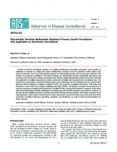
First, we show in Figure 1 the sequence plot of the
0 10 20 30 40 50 60
series itself, called Y From visual examination alone,
8.25+
we see that the series is obviously out of control, with
strong evidence of positively autocorrelated behavior
Y~ -t
(see also Box and Jenkins 1976, pp. 178-187). The sam-
- -- aL
ple mean is 7.06 and the sample standard deviation is
.40, so conventional three-sigma control limits would
extend from 5.86 to 8.26, limits that are shown in Figure
6.00+
1 only for illustration. All points are within these limits 60 70 80 90 100 110 120
(the maximum is 8.2 and the minimum is 6.1). (If the 8.25+
Y
data are viewed without regard to time sequence, they
-.-------
conform very closely to the normal model, providing
another illustration of nonrandom but approximately
6.75+
normal data.)
- LCL
IJ,=;
8.25+
Y .+ + + . + + +S QUEE
120 130 140 150 160 170 180
7. 50+
8.2+ 2
y - -A ---6.75+
7.50+
- - -- ---CL
6.00+ rrr
6.75+
+ + + + + + + 60SECUE
0 10 20 30 40 50 60
;L
8.25+ .L
6.00+
+ + +SEQUENCE
180 190 200
7. 50S
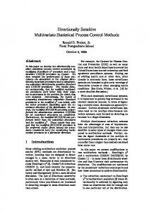
Figure 2. Sequence Plot of the Same Data as in Figure 1. UCL
6.75.
and LCL are limits computed from the mean of moving ranges of
successive observations.
6.00+ LCL
. + + . + + + SEG0U,
60 70 80 90 ?00 lio ao0 It is seen not only that the data are positively auto-
8.25+ UCL correlated, but that it is not even obvious that the data
Y-
7. 50+
Even if the process were deemed stationary, however,
three-sigma limits should logically be based on the mar-
6.75.
ginal rather than the conditional standard deviation.
Any concern with control limits, however, diverts at-
6.00+
+ ++^ tention from the basic observation that the conditional
120 130 140
mean is changing constantly. These changes of the con-
8.25+ -UCL
ditional mean are essential to understanding and control
of the process.
7.500+ r ~0-
A common approach for dealing with nonrandom
data like these is to base control limits on the mean of 6.75+
moving ranges of successive observations (Wadsworth
et al. 1986). We see in Figure 2 that these limits are 6.00+
LCL
++ + +GSEGU CE much tighter and show many points out of control, oc180 190 200
curring mainly at the peaks and troughs of the waves
Figure 1. Sequence Plot of
197 Concentration Readings or
Series A, Box and Jenkins (1976): of the data.
n a Chemical Process, Single Read- These control limits based on moving ranges alert the
ings Taken Every Two Hours.
Data are coded by subtraction of a
constant 10 from each observa
ition. CL is e eer e the center line at a height user that the process is not close to being random, but
equal to the sample mean, anc
I UCL and LCL show the location of they provide no real guidance in understanding what is
conventional three-sigma contr
.ol limits. happening.
This content downloaded from 143.88.93.232 on Fri, 04 Mar 2016 20:32:22 UTC All use subject to JSTOR Terms and Conditions
92 Journal of Business & Economic Statistics, January 1988
For many users, data like these suggest a series of
Y, is 0. As estimated by the Minitab ARIMA procedure,
we have
loosely connected episodes, each inviting ad hoc expla-
nations. (This parallels the after-the-fact "explana-
Fitted Y, = Yt_1 - .705A,_1.
tions" offered by stock-market analysts to "explain"
changes of the Dow-Jones Industrial Index!) The pro-
The quantity .705 is an estimate of what is called 0 by
cess of achieving a state of statistical control is some-
Box and Jenkins; 1 - .705 = .295 is an estimate of
times pictured as finding special explanations for each
what is often called a in discussions of the EWMA. The
episode, making a correction, observing the process
standard error of the estimated 0 is .05, and the standard
further, finding further special explanations for further
deviation of residuals is .318. (We have suppressed the
episodes, and so forth, until control is finally attained.
constant term, for two reasons: We have judged such
Here, however, as in the example of the Dow-Jones
a term unlikely a priori, and the sample evidence sug-
Industrial Index, simple time-series modeling unifies
gests an estimated constant near 0.)
the picture immediately.
Box and Jenkins fitted two models, each of which
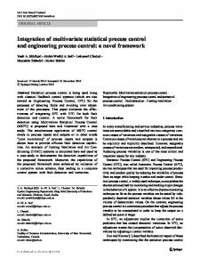
5.1 Common-Cause Chart: Fitted Values
describes the data about equally well. We consider one
It is useful to display the fitted values or estimated
of these models (the model underlying EWMA), namely
conditional means of the process, called "FITlED" in
a first-order integrated moving average, called "AR-
Figure 3, on a time-sequence plot. This plot gives a
IMA(0,1,1)," which, as pointed out previously, can be
view of the level of the process (estimated conditional
interpreted as a random-walk trend plus a random de-
mean) and of the evolution of that level through time.
viation from trend. This model specifies that the ob-
We see the systematic behavior of the process that per-
served Yt is the sum of an unobserved random shock
vades the entire period of observation. This behavior
A, plus a (proper) fraction a of the sum of all past
may aid in real-time control or in better understanding
random shocks A,_ , At-2, .... In the current appli-
how the process is working.
cation we have assumed that the mean of changes of
The model just fitted can be interpreted as follows:
Each observation can be thought of as a random dis-
turbance plus a random-walk trend or drift that reflects
FITTED -
a certain fraction of the sum of all past random distur7.50+ 9
bances. Thus a part of each disturbance continues to
affect the process into the indefinite future. The fitted
7.00+
values in Figure 3--P'lED-are estimates of the un-
6.50+
derlying random-walk trend; they follow a random walk
without drift. The chart of FI'IT'ED represents the first
+ + + + + + + SEC.CE
0 10 20 30 40 50 60
of the two charts proposed by us. Each point is an
FITTED -
estimate of the local level of the process itself, as dis7.50+
tinguished from the observed readings.
CL To illustrate the type of control decisions that could 7. O0 1 e
be based on this plot, suppose that the most desirable
level of the process is 7.0, and that increasing deviations
6.50S
from that level entail increasing economic loss from less+ 4 + + + +4 *SEQUENCE
60 70 80 90 100 110 120
than-optimal product. Suppose further that at a certain
FITED -
known cost it is possible at any time to recenter the
7.50+
process 7.0. Then one can make an economic calcula-
tion to balance the expected loss of bad product over 7.00+
some specified period of time against the cost of re-
centering. This calculation will define action limits both 6.50+
below and above 7.0 at which the process should be + + + + + + SEQUEiCZ
120 130 140 50 160 170 180
recentered.
FITTEDNote that these action limits are conceptually differ-
7.50+
ent from traditional control limits. They are not signals
- CL
that it is time to look for special causes; rather, they
7.00+
are signals that a specific corrective action is needed.
6.50+
+ + +SEQUECE
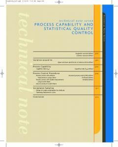
5.2 Special-Cause Chart: Residuals
i80 190 200
The second graph is essentially a standard control
Figure 3. Common-Cause Chart: Sequence Plot of Fitted Values
chart for residuals. To facilitate visualization of control for the Data of Figures 1 and 2. Estimates are based on the AR-
IMA(O, 1,1) model with 0 constant.
limits, we plot in Figure 4 the standardized residuals
This content downloaded from 143.88.93.232 on Fri, 04 Mar 2016 20:32:22 UTC All use subject to JSTOR Terms and Conditions
93
Alwan and Roberts: Time-Series Modeling for Statistical Control
ST.S For many purposes of control, whether real-time con-
2.50+
trol or process surveillance, either would be suitable.
From a theoretical point of view, the two models have
very different implications for the long-run behavior of
the process, assuming continuation of the basic condi-
tions now being observed. ARIMA(0,1,1) is nonsta-
0 10 80 30 40 50 60
tionary, but ARIMA(1,0,1) is stationary. Given the
STRES ARIMA(0,1,1) fitted previously, there is no tendency
0.00+ a. so*
of the process to revert to its mean level as it wanders
away. Given the ARIMA(1,0,1) for the same process,
there is a relatively weak tendency to mean reversion.
Moreover, prospective control limits as we look farther 2.50+
into the future are constant for ARIMA(1,0,1) but ever
0.00+
widening for ARIMA(0,1,1).
At one time we contemplated the concept of a sta-
tionary process as a possible extension of the concept
O ._~~~~- O O4CLU+LCL
of iid in defining a state of statistical control. The pres-
ent example illustrates, however, that data may not
permit a sharp distinction between stationary and non-
-a.50.0.00+ -
- ~ ~~~~- LC.~~~~~LCL
stationary. Hence we propose only that some time-se-
++ + + + SEEUECCE
810 t30 140 160 170 180
ries model be used to define statistical control in an
STRES) with approximate center line and upper and
extended sense. Even a nonstationary model permits
2.5 UL0+ probabilistic prediction.
Of course, if the weight of statistical evidence and
background knowledge suggests that the process should 0- t t t tt
be regarded as nonstationary, the problem confronting
-2.50+
LCL management is inherently more difficult, since a non-
+ +? + SENCE
180 190 200
stationary process has no tendency toward mean re-
version. For example, a stationary ARIMA model about,
Figure 4. Special-Cause Chart: Sequence Plot of Residuals for
say, a linear trend suggests disaster in the absence of
the Data of Figures 1 and 2. Estimates are based on the AR-
intervention. At the same time, the chart of residuals IMA(O, 1,1) model with 0 constant.
could suggest that special causes are occurring along
the road to ruin of the process itself.
(STRES) with approximate center line and upper and
lower three-sigma limits.
It is seen that two individual points-observations 43
5.4 Applications in Business and Economics
and 64-breach the three-sigma limits. By contrast, the
We have used a "public" data set to illustrate the
first set of control limits calculated previously suggested
mechanics of our basic proposals in an application that
no points out of control, but the second set, based on
will be familiar to many readers. Even here, however,
mean ranges, suggested many individual points out of
it results in identification of apparent out-of-control
control. These out-of-control points did include obser-
points that are easy to miss given the generally satis-
vation 64, which was at the top of a wave, but not
factory fit by ARIMA models.
observation 43.
We have had substantial experience in applications
In addition, the preceding plot reveals perhaps two
to business and economics, and these have confirmed
or three short intervals for which run counts would
the fruitfulness of time-series modeling. One interesting
suggest some suspicion of lack of control. Note that run
illustration is based on a report by BaRon (1978), who
counts are applied only after the residuals from the
studied the number of air tourist arrivals in Israel by
time-series model have been isolated. As applied to the
months for 20 years starting in January 1956. Except
original series, run counts would suggest that the proc-
for an upward trend and seasonality, BaRon's data con-
ess was nearly continually out of control, sometimes on
veyed the same visual general impression as the series
the high side and sometimes on the low side.
presented previously. Based on observation of the data
and knowledge of the historical background, BaRon
5.3 Other Simple Models
classified the 240 months into 26 segments of varying
The ARIMA(0,1,1) model fitted previously is not the
lengths; for example, segment 9 extended from Feb-
only reasonable model for the data. Box and Jenkins
ruary 1961 to July 1962. Within these segments, he used
also fit ARIMA(1,0,1) with a nonzero constant. The
three subclassifications: "regular," "short monotonic,"
two models give nearly identical fitted values and re-
and "unusual." February-December 1961, for exam-
siduals and hence about the same degree of overall fit.
ple, was identified as "unusual," and labeled "Eichman
This content downloaded from 143.88.93.232 on Fri, 04 Mar 2016 20:32:22 UTC All use subject to JSTOR Terms and Conditions
94 Journal of Business & Economic Statistics, January 1988
trial: disturbed growth," whereas January-July 1962
was "regular." BaRon also picked out nearly 40 "ex-
treme" months.
Although there can be no completely satisfactory sub-
stitute for statistical skills in time-series analysis, we
believe that much can be accomplished by people with
In a discussion of BaRon's paper, Roberts (1978)
reported that the series could be well fitted by a mul-
tiplicative seasonal model (0,1,1) by (0,1,1)12 on the
logs, with a constant term. Only one residual turned up
as an unmistakable outlier, and that was for the month
of October 1973-the Yom Kippur War. The model
limited skills. For example, modern computational tools
make possible relatively automated implementation of
time-series modeling; automatic fitting of Box-Jenkins
models has for some time been available in software of
general purpose software packages like Minitab, Stat-
graphics, SCA, or Systat now available on the IBM PC
itself is the so-called "airline" model used by Box and
and compatibles. [There are even programs that at-
Jenkins (1976) to fit a monthly time series of interna-
tempt to automate model identification, as well as fit-
tional airline passenger travel from 1949 to 1960. This
ting! See, e.g., Shumway (1986).]
suggests that many common causes underlying BaRon's
data were similar to those underlying foreign travel
worldwide and that special causes were rare.
Our approach has also been used by several hundred
students in the Executive Program and other programs
of the Graduate School of Business at the University
of Chicago who have applied it to data arising in various
areas of organizations for which they worked, ranging
from finance and marketing to production and research
and development. These applications typically find sys-
It is reassuring to know that precise model identifi-
cation may not be essential to effective process control;
several alternative models may fit the past data, at least,
about equally well. In particular, the two models men-
tioned in our example in Section 5-ARIMA(1,0,1) and
ARIMA(0,1,1)-offer reasonably good fit for a wide
range of applications. (As one referee has suggested,
the EWMA model may be a good all-purpose starting
point.)
If a process can be modeled, then the traditional
tematic time-series variation, including autocorrelation,
objectives of quality control-or surveillance-can be
seasonality, and trend. Many of them also find at least
better served. Moreover, a control mechanism can be
one outlying residual, and most of these students are
designed, and if a principal disturbance to the process
able to identify plausible special causes for these resid-
can also be modeled, we have the adaptive control sit-
uals.
uation described by Box and Jenkins (1976).
Typical examples are a sudden decrease in mean of
length of stay in a hospital, which was traced to the
7. ENGINEERING AND ECONOMIC ISSUES
imposition of the diagnostically related groups program;
More difficult than model identification and fitting is
an extreme negative bank stock return related to a pub-
the interpretation and exploitation of fitted values for
lic announcement of a write-off of nonperforming loans;
real-time process control, especially when process re-
a sharp decline in company sales of a capital-equipment
centering is costly, and for better understanding of un-
manufacturer in the third quarter of 1980, subsequently
derlying common causes that make the process behave
traced to the lagged effects of the economic recession
as it does. Real-time process control has received con-
that had occurred earlier in the year; a time-of-day
siderable attention, for example, by Box and Jenkins
effect in the occurrence of computer crashes; and an
(1970) and Box, Jenkins, and MacGregor (1974). Sys-
extremely high reading of hardness of steel coils, traced
tematic study of common causes has attracted little at-
to a scheduling error by which a billet of mixed steel
tention. We hope, in future work, to examine questions
was inadvertently processed into a coil.
like these in some detail.
One interesting economic illustration encountered by
several students from a variety of perspectives was the
ACKNOWLEDGMENTS
great increase in volatility of interest rates starting in
the fall of 1979, for which the special cause appears to
be a change of policy by the Federal Reserve System,
We are indebted to two referees and an associate
editor for many excellent suggestions.
a switch in emphasis from targeting interest rates to
[Received November 1986. Revised March 1987. targeting monetary aggregates.
6. TIME-SERIES MODELING IN PRACTICE
REFERENCES
A practical limitation on the use of the approach
BaRon, Raphael Raymond V. (1978), "The Analysis of Single and
advocated in this article is that implementation requires Related Time Series Into Components: Proposals for Improving
some skill in analysis of time series, whereas the imX-11," in Seasonal Analysis of Economic Time Series (Proceedings
plementation of the standard Shewhart procedures en-
of the Conference on the Seasonal Analysis of Economic Time
Series, Washington, DC, Sept. 9-10,1976), Washington, DC: U.S. tails only the most elementary statistical knowledge. We
Department of Commerce, Bureau of the Census, pp. 107-158,
believe that in many applications, the ability better to
171-172.
sort out special causes from common causes justifies Berthouex, P. M., Hunter, W. G., and Pallesen, L. (1978), "Moni-
the use of the more elaborate machinery required by toring Sewage Treatment Plants: Some Quality Control Aspects,"
our approach.
Journal of Quality Technology, 10, 139-149.
This content downloaded from 143.88.93.232 on Fri, 04 Mar 2016 20:32:22 UTC All use subject to JSTOR Terms and Conditions
Alwan and Roberts: Time-Series Modeling for Statistical Control
Box, G. E. P., and Jenkins, G. M. (1976), Time Series Analysis,
Forecasting and Control (2nd ed.), San Francisco: Holden-Day.
Box, G. E. P., Jenkins, G. M., and MacGregor, J. F. (1974), "Some
95
Page, E. S. (1954), "Continuous Inspection Schemes," Biometrika,
41, 100-115.
Roberts, Harry V. (1978), Comment on "The Analysis of Single and
Recent Advances in Forecasting and Control: Part II," Applied
Related Time Series Into Components: Proposals for Improving
Statistics, 23, 158-179.
X-11," by R. R. V. BaRon, in Seasonal Analysis of Economic Time
Deming, W. E. (1982), Quality, Productivity and Competitive Posi-
tion, Cambridge, MA: MIT Center for Advanced Engineering Study.
Eisenhart, Churchill (1963), "Realistic Evaluation of the Precision
and Accuracy of Instrument Calibration Systems," Journal of Re-
Series (Proceedings of the Conference on the Seasonal Analysis of
Economic Time Series), Washington, DC: U.S. Department of
Commerce, Bureau of the Census, pp. 161-170.
Shewhart, W. A. (1931), Economic Control of Quality of Manufac-
search of the National Bureau of Standards, C-Engineering and
tured Product, New York: Van Nostrand. (Republished in 1981,
Instrumentation, 67, 2.
with a dedication by W. Edwards Deming, by the American Society
Hoadley, B. (1981), "The Quality Measurement Plan," Bell System
Technical Journal, 60, 215-271.
Hunter, J. S. (1986), "The EWMA," Journal of Quality Technology,
18, 4.
Montgomery, Douglas C. (1985), Introduction to Statistical Quality
Control, New York: John Wiley.
for Quality Control, Milwaukee, WI.)
Shumway, R. H. (1986), "AUTOBOX (Version 1.02)," The Amer-
ican Statistician, 40, 299-300.
Wadsworth, Harrison M., Stephens, Kenneth S., and Godfrey, Blan-
ton A. (1986), Modern Methods for Quality Control and Improve-
ment, New York: John Wiley.
This content downloaded from 143.88.93.232 on Fri, 04 Mar 2016 20:32:22 UTC All use subject to JSTOR Terms and Conditions