1999, 71, 293–301
JOURNAL OF THE EXPERIMENTAL ANALYSIS OF BEHAVIOR
NUMBER
2 (MARCH)
TIME, TRACE, MEMORY J. E. R. S TADDON , J. J. H IGA , I. M. C HELARU
AND
DUKE UNIVERSIT Y AND TEXAS CHRISTIAN UNIVERSIT Y
Objections to a trace hypothesis for interval timing do not apply to the multiple-time-scale (MTS) theory, which incorporates a dynamic trace tuned by the system history and can easily accommodate interval timing over a 1,000:1 range. The MTS model can also account for Weber’s law as well as systematic deviations from it. Contrary to our critics, we contend that patterns of variance in interval timing experiments are not fully described by scalar expectancy theory, and that attempting to understand timing by assigning variance to different elements of a flexible model that lacks inductive support is a flawed strategy, because the attempt may be successful even if the model is wrong. We further argue that biological plausibility is an unreliable guide to the development of behavioral theory, that prediction is not the same as test, that induction should precede deduction, and that a rat is not a clock. Key words: interval, habituation, dynamics, multiple time scale, scalar expectancy theory, rat, pigeon
The line of argument often pursued throughout my theory is to establish a point as a probability by induction and to apply it as hypotheses to other points and see whether it will solve them. (Charles Darwin, ‘‘M’’ Notebook, p. 31) What we got heah, is a failyuh to communicate. (Strother Martin in Cool Hand Luke)
We thank the commentators for agreeing to respond to our paper. Our general aim was to open up the issue of interval timing: to expand the data set addressed by theories and to expand the range of theories deemed worthy of consideration. In this, we seem to have succeeded. Our specific aims were to point out the limitations of scalar expectancy theory (SET) and to show the advantages of the multiple-time-scale (MTS) approach. Here our success was not complete. Several commentators seem persuaded by our arguments against pacemaker-accumulator models and are willing to entertain an alternative; a few are noncommittal, but at least two strongly disagree. Nevertheless, even our severest critics concede that ‘‘SET would not be in any consequential way altered if the Poisson pacemaker assumption were abandoned’’ (Gallistel, p. 266) and ‘‘The key features of We thank Mark Cleaveland, Valentin Dragoi, and George King for comments on an earlier version. Research supported by grants to Duke University from NIDA and NIMH. Address correspondence to J. E. R. Staddon, Department of Psychology: Experimental, Duke University, Durham, North Carolina 27708 (E-mail:
[email protected]).
the theory did not rely on the Poisson pacemaker idea’’ (Gibbon, p. 272) In other words, the pacemaker is redundant, as we claim— and this was apparently known at the outset. The two major proponents of SET are unimpressed by the MTS theory. We address first their main objections to MTS: that no trace-decay theory of interval timing can possibly work; that MTS cannot make the kinds of detailed, quantitative predictions that are the major strength of SET; that we have failed to deal adequately with the time-left-experiment disproof of nonlinear time encoding; and that we have ignored the whole issue of variability and its incorporation into interval timing models. We conclude with remarks on some of the more general philosophy-of-science issues raised by the commentators. We apologize in advance to the majority of our commentators: We agree with most of what they say and so have little response beyond ‘‘Amen!’’ In the limited space available, we respond mostly to our critics. Can Inter val Timing Be Explained by a Trace? Gallistel writes that ‘‘Scalar variability [i.e., the Weber law property of interval timing]. . . appears to be irreconcilable with the assumption that temporal intervals are measured by a decay process, which is the central assumption in Staddon and Higa’s model’’ (p. 271). Based on lengthy calculations derived from our Figure 1, he argues (and Gibbon agrees) that at long times, our traces are ‘‘effectively zero’’ (p.
293
294
J. E. R. STADDON et al.
270), so the model cannot provide an accurate picture of interval timing over a realistic (1,000:1) range. These are damning criticisms, and they rule out a fixed-trace model. But both are false for the tuned trace intrinsic to the MTS model, as we explained in the paper, as Killeen explains in his commentary, and as we now explain again, with a picture. Figure 1 shows how the trace is tuned by different histories. In this simulation a 10-unit MTS model (Figure 4 in Staddon & Higa shows a single unit; 10 of these were cascaded in the simulation) was exposed to a long series of constant stimuli at fixed interstimulus intervals (ISIs) ranging from 5 to 5,000 time steps. The left column of panels shows the trace values for each of the 10 integrators at the end of each series. Notice that at short ISIs, only early (hence faster) units are active, whereas at longer ISIs, later (hence slower) units also become active. The result is that the trace decays rapidly in extinction after a history of closely spaced stimuli but does so slowly after a history of widely spaced stimuli. An MTS model with a sufficient number of units can therefore accommodate interval timing over any specified range. For a range of 1,000:1, about 10 units are sufficient. Because all these extinction functions decay rapidly at first and more slowly thereafter, each of them can be reasonably well fit by a power function, although the parameters will be different for each fit. Each power function will be effectively zero after a long enough time, but that time will be directly related to the ISI during training. Thus, any specific experiment (such as those carried out by Stubbs and his associates, discussed in our paper) can be modeled reasonably well either by a power-function trace or by MTS, as we claim in the paper. Can the MTS Model Account for Scalar Timing? The scalar (Weber law) property is an important property of interval timing. Nevertheless, Gallistel’s enthusiasm for what he terms time-scale invariance goes well beyond what the data will support. Many experiments, notably those by Zeiler and by Stubbs and his associates, do not fit this scheme. The data of Dreyfus, Fetterman, Smith, and Stubbs (1988), for example, show pretty clearly that time ratios alone do not explain relative-choice data: Pigeons are better at discriminating 10 s from
20 s than discriminating 20 s from 40 s, a violation of time-scale invariance. Interval size does matter; ratios are not everything, as we point out at some length in the paper. Scalar variance is assumed, rather than explained, by SET. Nevertheless, no theory that fails to accommodate the Weber law property of interval timing, at least approximately, is likely to be taken seriously. Figure 2 shows that a 10 habituation-unit cascade, together with simple assumptions about start and stop response thresholds and fixed (not scalar) Gaussian variance, can match prototypical peak-procedure scalar timing data. To simulate these data, we set up a structure comparable to SET; that is, a process whereby a ‘‘remembered time’’ (stored trace value) is compared with the current time (current trace value) and responding is driven by thresholded comparison between them (cf. Staddon & Higa, Figure 3). We do not like this as a general approach to interval timing, because it is very much restricted to the peak procedure, cannot (because of the all-ornone response rule) accommodate fixed-interval (FI) scalloping, and does not deal in a natural way with timing of multiple intervals (e.g., as on mixed- and variable-interval schedules; see Church’s comment). Nevertheless, it is the scheme used by SET, and it seems fair to use it when defending ourselves against charges that the MTS model ‘‘does not derive the observed scalar variability from more basic assumptions. Indeed, it does not even provide an explanation of the observed scalar variability’’ (Gallistel, p. 266), that ‘‘although the article contains 21 equations, there is no quantitative comparison of observed with predicted behavior’’ (Church, p. 255), and that our model is ‘‘never addressed to real data’’ (Gibbon, p. 272; we assume that Gibbon means quantitative data, because much of the paper is devoted to qualitative data). So we here follow the suggestion at the end of Church’s commentary ‘‘to substitute the output of a series of cascaded habituation units for a pacemaker-accumulator system in scalar timing theory. . . . This would provide a basis for a quantitative comparison of the two models’’ (p. 255). To generate the simulated data in Figure 2 we assumed first that the system learns the currently reinforced trace value, VM* (cf. Equation 18 in the paper), termed STM* in the simulation, according to
REPLY
295
Fig. 1. Left panels: Steady-state integrator V values for a 10-unit habituation cascade after a history of stimulus presentations at interstimulus intervals ranging from five time steps (top) to 5,000 (bottom). These are the initial conditions at the beginning of extinction. Right panels: Memory trace (sum of V values) in extinction, after the training series. The longer the ISI during training, the more integrators are active and the slower the trace decay. Note the resemblance between the pattern of integrator activation at different ISIs and the SQUID data reported by Williamson (Glanz, 1998). The decay parameters (Equation 16 in Staddon & Higa) for the 10 integrators were set according to the rule ai 5 1 2 exp(2li), where l 5 .9 (with this l value, the Weber fraction estimate approximately doubles over the 5 to 5,000-s range); bi 5 .2.
LTM(k 1 1) 5 LTM(k) 1 X(k)[STM(k 2 1) 2 LTM(k) 1 mz(k)],(1) where k is the time step, LTM is the remem-
bered value of the trace, X is the current value of reinforcement (usually 1 or 0), STM is the current trace value, z(k) is Gaussian noise with zero mean and unit standard deviation,
296
J. E. R. STADDON et al.
Fig. 2. MTS simulation (S) of peak-interval procedure peak-rate data (D) from Church, Meck, and Gibbon (1994, Figure 3), 240-s ‘‘empty’’ trial condition with a 30-s ITI. Symbols: Data. Solid lines: MTS simulation. Model: The system learns the value of the trace that is currently associated with reinforcement, STM* (stored as LTM). Responding then begins when the trace declines below a start threshold above LTM, and ceases when it falls below a stop threshold below LTM. For this simulation, the start and stop thresholds were LTM 1 .05 and LTM 2 .015, respectively; ai values were set as in Figure 1 with l 5 .9 and bi 5 .2; noise (parameter m in Equation 1) was Gaussian with standard deviation 0.02; 1 s 5 eight time steps. The simulation is based on 1,024 trials.
and m, the single parameter, is the noise weight. In words, the remembered reinforced trace value, LTM, is set to the currently reinforced trace value, STM*, with added noise. In the absence of reinforcement (X 5 0), LTM remains the same. Second, we assumed that responding occurs at a constant rate as long as ustop , STM , ustart. In words, the system responds at a constant rate as long as the current trace value is in between the start and stop thresholds. Third, we assumed that the start and stop thresholds are fixed amounts above and below the reinforced trace memory, LTM: ustart 5 LTM 1 kstart; ustop 5 LTM 2 kstop. This scheme has five free parameters: the two thresholds, l (the rate of increase of time constants across the cascade), b, and the noise weight, m—not particularly parsimonious, but no worse than SET. And this version of our model includes an explicit, real-time learning rule, which SET does not. Figure 2 shows that the same set of parameters produces a tolerable fit to group-average peakrate histograms for three peak-procedure conditions (15, 30, and 60 s) and does so while assuming fixed thresholds and constant, not scalar, variance. This simulation refutes Gallistel’s assertion that ‘‘the observed distributions are not predicted by a model
that assumes that (a) the relation between subjective intervals and objective intervals is . . . determined by a decay process and (b) the noise in a subjective interval is Gaussian with constant standard deviation’’ (p. 270). We should emphasize that Figure 2 is intended to show that the MTS model can generate quantitative predictions in the manner of SET, if we accept the same constraints as SET, namely an all-or-none response rule and free parameters that are not linked to schedule parameters, plus a simple learning rule. Equation 1 is simpler than the sampling system for interval learning that has been proposed for SET (e.g., Brunner, Gibbon, & Fairhurst, 1994; Gibbon, 1991) but it is only marginally more satisfactory in its ability to provide an account of true dynamic timing effects (e.g., Lejeune, Ferrara, Simons, & Wearden, 1997). The assumptions that underlie the simulation in Figure 2 are far from adequate. Only when we have full confidence in the whole model structure, including the learning process, can issues related to variance be decided (see below). Does the Time-Left Procedure Imply Linear Time Encoding? Both Gibbon and Gallistel argue that the time-left procedure, particularly the two-stan-
REPLY dard version, conclusively refutes the idea of log-like nonlinear time encoding. The proof offered is that when comparing an elapsing delay to two unpredictable delays, the point of indifference is at the harmonic mean of the pair (Gallistel, p. 265). There are four things to note about this conclusion. First, the data are far from novel. Killeen (1968) found the same thing in a choice experiment in which pigeons chose between two two-link chained schedules. One final link was fixed, and the other was two equiprobable fixed intervals. Killeen concluded that ‘‘relative amount of responding in the initial link equaled the relative harmonic rate of reinforcement in the terminal links’’ (p. 263). Hence, pigeons are indifferent between a fixed-interval second link and a two-interval second link with the same harmonic-mean interval. Second, the experimental issue is the different averaging processes implied by the bisection experiment (which shows geometric-mean averaging and implies log-like time encoding) and the time-left experiment (which shows harmonic-mean averaging and implies linear time encoding). But these two procedures are quite different. In the bisection experiment the animal responds left or right depending on the duration of a sample stimulus. In the time-left experiment, the animal responds left or right depending on an expectancy—what it has learned about the upcoming reinforcement rates associated with each choice at that time. It should not surprise us if these very different procedures yield very different results. Third, Killeen’s result has usually been interpreted as telling us something about how pigeons in effect compute rates of reinforcement. Given a set of interreinforcement intervals t1, t2, . . . tN, reinforcement rate is computed by the animals according to 1/(t1 · t2 · . . . · tN)1/N rather than N/(Sti) (i.e., the harmonic rather than the arithmetic mean). There is no necessity for any timing process here, because rates can be computed in ways that do not require the explicit learning of time intervals, for example, by an integrator or appropriate differential equations (cf. Dragoi & Staddon, in press). Fourth, given that animals assess expected rates of reinforcement by means that have no necessary relation to time encoding, patterns of preference for stimuli associated with different reinforcement rates have no
297
necessary bearing on the issue of how time is in fact encoded. Translated to the two-standard time-left procedure, Killeen’s result means that the animal must compare a rate of reinforcement equal to the reciprocal of the harmonic means of the two unpredictable standard delays with expected rates of reinforcement at different elapsed times since trial onset on the time-left key. What the animal must learn, therefore, is the particular value of encoded in-trial time, t, at which the expected rate of reinforcement on the timeleft key is equal to the expected (harmonicmean) rate of reinforcement on the standard key. The fact that the animal can learn this task tells us nothing about how t is encoded, other than that it is monotonic with real time (i.e., that there exists a unique value of t for which both expected rates of reinforcement are equal). The fact that the value of t at which the animal is indifferent corresponds to a time to food equal to the harmonic mean of the set of variable standards tells us, again, that expected reinforcement rate is computed harmonically, not arithmetically or geometrically. Proponents of the time-left procedure might reasonably ask, ‘‘Well, if you don’t accept the SET interpretation of the relation between time discrimination and the computation of reinforcement rate, what can you offer in its place?’’ Fair enough; we have no firm alternative, although in our discussion of the consequences of Equations 8 and 9 in the text we suggest one possibility. But we do contend that because reinforcement rate can be computed in ways that are independent of the processes of explicit time estimation, the time-left experiment will not bear the theoretical weight that has been placed upon it. In particular, it cannot be used to refute the idea that time is encoded nonlinearly. What Is the Proper Role of Variability in Behavioral Models? This question is at the heart of the criticisms of our paper by our chief critics. Gibbon says that ‘‘there is no talk of variance throughout [their] paper’’ (p. 274), and Gallistel says that ‘‘The Staddon and Higa proposal offers no explanation for the observed variability, and it is unclear what noise assumption would yield the observed variability’’ (p. 264). We have just described an as-
298
J. E. R. STADDON et al.
Fig. 3. Normalized waiting-time (start-time) distributions from a single pigeon long-trained on several responseinitiated delay schedules. Clamped refers to an FI-like schedule in which the time between reinforcers is held constant; fixed refers to schedules in which the delay, T, is constant. The distributions roughly superimpose, consistent with Weber’s law, and are symmetrical on a log scale. (Reprinted from Wynne & Staddon, 1988, Figure 5)
sumption that would yield the obser ved variability, but Gibbon and Gallistel are correct that we avoided doing so in the paper. There are two reasons we neglected variance, one specific and the other more general. The specific reason is that the ability of SET to deal with variability is not as well established as our critics imply. Most discussion is devoted to peak-rate distributions, such as those shown in Figure 2, which are generally Gaussian, symmetrical, scalar, and centered on the time of reinforcement—although there are some exceptions, as we point out in the paper (Cheng & Westwood, 1993; Zeiler & Powell, 1994). But data on start and stop times, in the peak procedure and in fixedinterval-type procedures, are not so simple. For example, Brunner et al. (1997, Figures 2, 8, and 11) report start-time data that are strongly skewed to the right, not symmetrical as SET would suggest. Admittedly, the definition of start in the peak procedure, and on FI, is somewhat ambiguous, but on response-initiated-delay schedules it is not. On response-initiated-delay schedules, the first response after reinforcement causes a stimulus change and initiates a delay, T, until the next reinforcement,
which requires no additional response. On so-called clamped schedules, the time between reinforcement is fixed, so that t 1 T is constant, where t is the wait (start) time until the first response (i.e., the procedure resembles an FI schedule). Start-time distributions on such procedures are symmetrical on a log (not linear) scale (see Figure 3), consistent with MTS but not with SET, absent assumptions about additional sources of variance (Brunner et al., 1994, p. 76). Start times are a simpler and more primitive measure of temporal discrimination than is peak-rate time. They are easier to collect and require less averaging. Yet they seem to be incompatible with SET. We need to see a comprehensive SET analysis of start and stop times, as well as more detailed treatment of start, peak, and stop times by MTS, before we can judge which approach really does a better job of treating variability. The general reason we omitted discussion of variance from our paper can be illustrated by an anecdote. When I (Staddon) was learning physics in high school from our bald, boring (but, in retrospect, very good) German physics master, we learned about sources of error in calorimetry, a topic not riveting to
REPLY 17-year-olds. Nevertheless, I still recall his discussion of the various means by which heat could leak away from the sample whose specific heat was to be measured: conduction, convection, radiation, and, perhaps, evaporation, were all sources of measurement error. Each of these processes could be demonstrated independently, and their properties were known. The physics of the whole situation had been independently established. It made sense, therefore, to partition the observed variance into these various known components. Translated to the behavioral context, the scientific question is: Are the laws of temporal discrimination in rats and pigeons well enough established that we can make with confidence assertions such as ‘‘this analysis was designed to attempt to isolate the relative contributions of memory and decision variance in this procedure’’ (Gibbon, p. 274)? That is, are the theoretical constructs ‘‘memory’’ and ‘‘decision process’’ as well established as ‘‘convection’’ or ‘‘radiation’’ so that it makes sense to assign components of variance to them? We contend that the answer to this question is a pretty firm “no.” The SET structure of which these are a part is not well enough established to make questions like this appropriate. Consequently, to set up the situation in this way is not to isolate sources of error in a known process—a familiar, legitimate scientific procedure—but rather to see if a variable and rather restricted data set can be fitted by injecting variance at various points in a hypothetical structure, which is much more questionable. It is a hazardous practice because if data are both variable and limited in scope, and if the theoretical structure is relatively flexible, a fit may be found, whether or not the structure is in fact correct. The first priority, most will agree, is to find the true structure. We believe that this cannot be done by looking chiefly at variance, for the reason just described: Given a relatively unparsimonious structure and a relatively restricted data set, it is simply too easy to generate quantitative fits, even if the structure is false. Gibbon points out that ‘‘a major thrust of psychophysics . . . has been to understand sources of variability and error’’ (p. 275), to which the snappy answer is ‘‘so much the worse for psychophysics.’’ A more measured
299
response is to point out first that there is greater consensus on the appropriate model in psychophysics. Second, in most psychophysical studies, averaging is within subject, not between subjects (see, e.g., Staddon, King, & Lockhead, 1980); consequently the ultimate aim of the inquiry, understanding mechanisms of behavior in the individual organism, is not compromised. Third, learning is not central to psychophysical problems, and the dependence of psychophysical performance on history is minimal. Even the venerable time error apparently has more to do with the form of the scale than the order of stimulus presentation (Stevens, 1975). Partitioning sources of variance in psychophysics may well be less misleading than in temporal discrimination. If not by analysis of variance, then how is interval timing to be understood? We address this question as part of a general discussion of philosophy of science. Philosophy of Science There is no litmus test for deciding between theories. Many believe there is a rule for deciding on data: ‘‘Fact’’ is often treated as synonymous with ‘‘significant at the 5% level,’’ for example. One of our commentators (Church, 1997) has suggested that there should be a similar algorithm for deciding which of two theories is ‘‘true.’’ But we believe both views are mistaken. The idea that truth—of a theory or of a datum—can be decided algorithmically is a myth. Explanation, prediction, test, and control. B. F. Skinner made much of science as the search for ‘‘prediction and control,’’ with emphasis on control. Others have laid more stress on the power to explain; and all agree that the essence of a scientific hypothesis is that it be subject to test. We claim that the truth of a theory may rest on any or all of these four legs, and the weight on each will depend on what the theory is and what it purports to explain. In experimental psychology, the greatest weight has always been placed on prediction and test, and much less on the power of a theory to explain a range of data. Psychologists are unfortunately much more impressed by a match, especially a quantitative match, between data and prediction than by any attempt to explain relations among disparate
300
J. E. R. STADDON et al.
data sets. But testing a prediction is not the same as testing a theory. Given a flexible theory and limited domain of data, a good predictive fit may be more or less guaranteed, as we contend is the case for SET. A true test of a predictive theory, on the other hand, would take the simplest and most fundamental assumption of the theory and evaluate it directly. We have tried to do this for both the pacemaker and the assumption of linear time encoding. We claim that there is negligible evidence for the pacemaker (despite 20 years of search) and inadequate evidence for linear time encoding. Because SET is primarily a predictive (rather than an explanatory) theory, the failure of one or more of its core assumptions calls the whole thing into question. But not all theories gain credence through experimental test. Darwinian evolution, for example, was until recently hardly testable at all. It gained adherents through its power to explain. Our defense of MTS theory, like Darwin’s defense of evolution by natural selection, rests on “establish[ing] a point as a probability by induction and applying it as hypotheses to other points to see whether it will solve them.” Our justification for MTS time encoding is that its central assumption, a cascade of tuned habituation units, has independent support from both behavioral (Staddon & Higa, 1996) and physiological (e.g., Glanz, 1998; Uusitalo, Williamson, & Seppa¨, 1996) habituation data on the one hand and human and animal memory data (Staddon, 1998) on the other. Unlike the idea of a linear internal clock, which is entirely a priori, the MTS model has some independent basis. It may be wrong as applied to interval timing (and the theory is certainly incomplete) but its power to explain a wide of range of experimental results gives it credibility that a pacemaker-accumulator system lacks. Parsimony. Parsimony is not just a desirable feature, like electric windows or a self-cleaning oven, it is the measure of explanatory power. Because parsimony cannot be defined exactly does not mean that it does not exist. (Beauty cannot be defined exactly either, but few doubt that Miss World is better looking than Godzilla.) As Killeen points out, parsimony is a ratio, composed of facts explained divided by assumptions made. The theorist has an equal obligation to reduce the denom-
inator (by stripping out unnecessary assumptions, like redundant, undetectable pacemakers) and add to the numerator (by applying the theory to the widest possible range of data, not just the peak-interval procedure and its variants). The parsimony of dynamic models can to some extent be measured. The denominator can be quantified in answer to two questions: How many state variables does the model have? How many free parameters are there? Both are important. For example, a neural net model may have very few free parameters, but because it has very many state variables (the synaptic weights) it can accommodate a wide range of data. Nevertheless, the ratio of data explained to state variables needed may be quite small, so that despite its power and the small number of free parameters, such models may not be very parsimonious, and not very explanatory. The numerator, the number of facts explained, is harder to quantify, but we can at least look at areas of overlap (data explained by both competing theories) as well as data explained by one and not the other. We would be inclined to give more weight to explaining the outcome of different experimental arrangements than to detailed fitting of data from one arrangement. On these grounds we tend to prefer MTS, which potentially looks at every operant situation that involves temporal control, to SET, which focuses on a limited number of experimental arrangements that can also (we believe, although this remains to be shown in detail) be explained by MTS. Biological plausibility. Gibbon, and Donahoe and Burgos, all give some weight to the idea that a proper timing model should be biologically plausible. We argue in the paper that this idea is mistaken, if only because biology is too rich to much constrain behavioral theorizing (there are other objections to this notion as a useful guide to theories of behavior; cf. Staddon & Bueno, 1991; Staddon & Zanutto, 1998). Donahoe and Burgos object to inferred process models, and consequently do not like either the SET or the MTS approach, although they agree with our contention that timing can occur in the absence of a pacemaker. Hence they present a biobehaviorally informed, but pacemaker free, neural net model.
REPLY Their approach has produced some interesting results, but it does not really live up to its underlying philosophy. First, theoretical neural networks are also inferred process models, to the extent that they model only certain aspects of neurons and not others. For example, it is not too common to see neural net models that include auto- and heteroreceptors and changes in membrane permeability, as well as the resulting changes in neurotransmitter synthesis and their effects on subsequent neuronal firing rates—not to mention field effects and circulating neurohumors. Neural models are always selective in just what neural properties they choose to incorporate. They are just as ‘‘inferred’’ as frankly formal models like MTS and early SET. Second, ‘‘neural’’ models are usually incomplete because our understanding of neurobiology is incomplete and evolving. For example, the Donahoe–Burgos model uses a dopaminergic system to adjust connection weights, probably because until recently most investigators viewed mesolimbic dopamine systems as the primary, if not the only, neurotransmitter involved in the neurobiology of reinforcement. However, recent research paints a more elaborate picture, which includes the idea of the extended amygdala, as well as recognizing the importance of other neurotransmitter systems such as glutamate and serotonin (cf. Koob & Le Moal, 1997). Models that aspire to be biologically correct need to be continuously modified in light of new biological research, a challenge that is rarely met. The Pygmalion fallacy. In Greek mythology the misogynist sculptor Pygmalion carved an ivory statue of a woman so beautiful that he fell in love with it. Operant conditioning sculpts behavior so effectively that there is a tendency to mistake the outcome of training for the thing itself. So, we can train a rat to behave like a clock, but we forget that it is after all not a clock, but a rat. The object of theory and experiment must still be to understand the rat, not the clock. REFERENCES Brunner, D., Gibbon, J., & Fairhurst, S. (1994). Choice between fixed and variable delays with different re-
301
ward amounts. Journal of Experimental Psychology: Animal Behavior Processes, 4, 331–346. Cheng, K., & Westwood, R. (1993). Analysis of single trials in pigeons—timing performance. Journal of Experimental Psychology: Animal Behavior Processes, 19, 56– 67. Church, R. M. (1997). Quantitative models of animal learning and cognition. Journal of Experimental Psychology: Animal Behavior Processes, 23, 379–389. Church, R. M., Meck, W. H., & Gibbon, J. (1994). Application of scalar timing theory to individual trials. Journal of Experimental Psychology: Animal Behavior Processes, 20, 135–155. Dragoi, V., & Staddon, J. E. R. (in press). The dynamics of operant conditioning. Psychological Review. Dreyfus, L. R., Fetterman, J. G., Smith, L. D., & Stubbs, D. A. (1988). Discrimination of temporal relations by pigeons. Journal of Experimental Psychology: Animal Behavior Processes, 14, 349–367. Gibbon, J. (1991). Origins of scalar timing. Learning and Motivation, 22, 3–38. Glanz, J. (1998). Magnetic brain imaging traces a stairway to memory. Science, 280, 37. Killeen, P. (1968). On the measurement of reinforcement frequency in the study of preference. Journal of the Experimental Analysis of Behavior, 11, 263–269. Koob, G., & Le Moal, M. (1997). Drug abuse: Hedonic homeostatic dysregulation. Science, 278, 52–58. Lejeune, H., Ferrara, A., Simons, F., & Wearden, J. H. (1997). Adjusting to changes in the time of reinforcement: Peak-interval transitions in rats. Journal of Experimental Psychology: Animal Behavior Processes, 23, 211– 321. Staddon, J. E. R. (1998). The dynamics of memory in animal learning. In M. Sabourin, F. Craik, & M. Robert (Eds.), Advances in Psychological Science: Vol. 2. Proceedings of the XXVI International Congress of Psychology (pp. 259–274). Hove, UK: Psychology Press. Staddon, J. E. R., & Bueno, J. L. O. (1991). On models, behaviorism and the neural basis of learning. Psychological Science, 2, 3–11. Staddon, J. E. R., & Higa, J. J. (1996). Multiple time scales in simple habituation. Psychological Review, 103, 720–733. Staddon, J. E. R., King, M., & Lockhead, G. R. (1980). On sequential effects in absolute judgment experiments. Journal of Experimental Psychology: Human Perception and Performance, 2, 290–301. Staddon, J. E. R., & Zanutto, B. S. (1998). In praise of parsimony. In C. D. L. Wynne & J. E. R. Staddon (Eds.), Models for action: Mechanisms for adaptive behavior (pp. 239–267). New York: Erlbaum. Stevens, S. S. (1975). Psychophysics: Introduction to its perceptual, neural, and social prospects. New York: Wiley. Uusitalo, M. A., Williamson, S. J., & Seppa¨, M. T. (1996). Dynamical organization of the human visual system revealed by lifetimes of activated traces. Neuroscience Letters, 213, 149–152. Wynne, C. D. L., & Staddon, J. E. R. (1988). Typical delay determines waiting time on periodic-food schedules: Static and dynamic tests. Journal of the Experimental Analysis of Behavior, 50, 197–210. Zeiler, M. D., & Powell, D. G. (1994). Temporal control in fixed-interval schedules. Journal of the Experimental Analysis of Behavior, 61, 1–19.