Robert A. Thacker Wendy Belluomini. Chris J. Myers. Computer Science Department ...... [8] J. R. Burch. Modeling timing assumptions with trace theory. In ICCD ...
Timed Circuit Synthesis Using Implicit Methods Robert A. Thacker Wendy Belluomini Chris J. Myers Computer Science Department Electrical Engineering Department University of Utah University of Utah Salt Lake City, UT 84112 Salt Lake City, UT 84112
Abstract The design and synthesis of asynchronous circuits is gaining importance in both the industrial and academic worlds. Timed circuits are a class of asynchronous circuits that incorporate explicit timing information in the specification. This information is used throughout the synthesis procedure to optimize the design. In order to synthesize a timed circuit, it is necessary to explore the timed state space of the specification. The memory required to store the timed state space of a complex specification can be prohibitive for large designs when explicit representation methods are used. This paper describes the application of BDDs and MTBDDs to the representation of timed state spaces and the synthesis of timed circuits. These implicit techniques significantly improve the memory efficiency of timed state space exploration and allow more complex designs to be synthesized. Implicit methods also allow the derivation of solution spaces containing all valid solutions to the synthesis problem facilitating subsequent optimization and technology mapping steps.
1. Introduction Recent trends in the integrated circuit industry, such as decreasing feature sizes and increasing clock speeds, make global synchronization across large chips difficult to maintain. As a result, many designers have become interested in asynchronous circuits because they eliminate the need for global synchronization. Asynchronous circuits consist of groups of independent modules which communicate using handshaking protocols. Since there is no global clock, clock distribution and skew are not issues. Also, eliminating the global clock permits modules to work at their own pace and allows average-case performance to be realized. There are a number of different styles for designing asynchronous circuits. Most asynchronous design methodolo-
�
This research is supported by NSF CAREER award MIP-9625014, SRC contract 97-DJ-487, an SRC Graduate Fellowship, and Intel Corp.
gies are based on the assumption that nothing is known about the delays between signal transitions. Therefore, the circuit must be constrained to work correctly even in cases which never occur in a realistic implementation. The overhead necessary to guarantee this behavior often makes the asynchronous average-case performance worse than the synchronous worst-case. Timed circuits are a class of asynchronous circuits which use explicit timing information in circuit synthesis. Precise timing relationships are often unknown before synthesis and technology mapping. However, applying even rough estimates can lead to the removal of large amounts of circuitry that would be required for a speed-independent design. These timing assumptions can then be formally verified after synthesis when the actual timing values are known. This design style can lead to significant gains in circuit performance over asynchronous circuits designed without timing assumptions [15]. The first stage of timed circuit synthesis involves the exploration of the timed state space to determine which untimed states are reachable by the system. The circuit is first specified using a formalism that allows a lower and an upper bound to be assigned to the causal relationships between signals. Timing analysis is then performed by our design tool ATACS using geometric regions and partially ordered sets (POSETS) of events, which has been shown to be an efficient method for representing information about timed state spaces [3, 4, 16, 17]. We use Binary Decision Diagrams (BDDs) [7] and Multi-terminal Binary Decision Diagrams [10] to efficiently represent these timed state spaces. The second stage of synthesis consists of repeatedly dividing the state graph into subregions to determine the necessary behaviors. For each signal, the graph is divided into those regions where the signal should be enabled to rise, should be enabled to fall, should remain high, or should remain low. Equations are derived to represent a circuit implementation which conforms to these behaviors. Our synthesis method uses BDDs allowing the derivation of solution spaces containing all valid solutions to the synthesis problem.
2. Timed state space exploration Timed circuit synthesis is dependent on a complete exploration of the timed state space of the specification. This state space can be very large since it must include, not only all of the combinations of signal values allowed by the specification, but also the time relationships between signal firings. However, it can be smaller than the complete state space of an equivalent specification without timing since states that are not reachable given the timing information are not explored. The size of the timing information depends on the timing algorithm being used. One representation is to attach a clock to each signal transition that advances only in discrete time steps [8]. This representation can cause state space explosion, especially for large delay ranges [17]. A BDD method has been proposed in [6], to improve discrete time memory performance, but it does not address the state explosion problem inherent in discrete time. The geometric region method, where timing information is stored as a constraint matrix representing relationships between signal transition times, has been shown to be an efficient way to represent a timed state space [3, 14, 16, 17]. However, even with a region based representation, the memory required to store such a state space explicitly can be prohibitive for large designs. In many domains, implicit methods have been shown to significantly reduce memory usage [7]. Since timed state space exploration is such a memory intensive process, it is an excellent candidate for such an approach.
������� ��
������� ���������������� �!� The block diagram in Figure 1 is for a controller for a self-timed FIFO. In [13], a highly optimized timed circuit implementation is presented which is designed by hand. The correctness of this circuit is highly dependent on timing parameters. This example is used to show how our timed circuit synthesis method can derive the same efficient circuit from the description of the required behavior and the known timing parameters. The basic behavior is that when a request comes in (i.e., FIN " ) and the fifo is empty (i.e., EOUT is high), the data is latched (i.e., En bar " and En # ). In parallel, the insertion is acknowledged (i.e., SEOUT # ) and the next stage is requested to accept the data (i.e., FOUT " ). When the next stage accepts the data (i.e., SEIN # ), the FIFO is set to be empty (i.e., EOUT " ) and the latch is opened (i.e., En bar # and En " ).
���$�%�'&(��� �!�!)*�$ + ������*,.-/ 0�� 0�1-2�3�4)5�6�����3�! 87��4 ��! 8�
En_bar
EOUT FOUT
FIN SEOUT_
SEIN_
Figure 1. Block diagram for a timed FIFO. formally in [2]. TEL structures can represent a set of specifications equivalent to those represented by both time and timed Petri nets, as well as others that are quite difficult to represent with a Petri net. A TEL structure consists of a set of rules that represent causality between signal transitions, or events, as well as a set of conflicts which are used to model disjunctive and choice behavior. Each rule is of the form 9$:=*;>?@;BA ;DCFE , where : is the enabling event, = is the enabled event, 9$?G;GA�E is the bounded timing constraint, and C is a boolean expression which must be satisfied before = is allowed to occur. A rule is said to be enabled if its enabling event has occurred and its boolean expression evaluates to true. The timing constraint places a lower and upper bound on the timing of a rule. A rule is satisfied if the amount of time which has passed since the enabling event has exceeded the lower bound of the rule. A rule is said to be expired if the amount of time which has passed since the enabling event has exceeded the upper bound of the rule. Ignoring conflict, an event cannot occur until all rules enabling it are satisfied. An event must always occur before every rule enabling it has expired. Since an event may be enabled by multiple rules, it is possible that the differences in time between the enabled event and some enabling events exceed the upper bound of their timing constraints, but not for all enabling events. A graphical representation of the TEL structure for the FIFO example is shown in Figure 2. Nodes represent signal transitions and arcs represent causal relationships between them. Tokens on arcs indicate that the preceding transition has occurred but the following transition has not. All incoming arcs must have tokens to fire a transition. The goal of state space exploration is to derive the state seoutb-/1
[90,110] fout-/1
[90,110]
[90,110] (fin & eout)
(~eout)|(~fin) seoutb+/1
foutb+/1
[180,260] (~seoutb)
foutb-/1
fout+/1 [180,inf] (seoutb)
[90,110] eout-/1
eoutb+/1
seinb-/1 [90,110] (~fout)
(eoutb&seinb)
[90,110]
fin+/1
[90,inf] (fout)
[90,110]
[90,110] (~seinb)
fin-/1
seinb+/1
The state space exploration procedure used by ATACS begins with a timed event/level (TEL) structure, described
En
[90,110]
[90,110] (~seoutb) eout+/1
eoutb-/1
(seoutb&foutb)
[90,110]
Figure 2. The TEL structure for the FIFO.
graph (SG), which is necessary for circuit synthesis. A SG is a graph in which the vertices are untimed states and the edges are possible state transitions. A transition between two states exists if the specification allows the circuit to move from one state to the other with one signal transition. A reduced state graph (RSG) is a SG where some branches have been pruned because timing information has shown them to be unreachable. A RSG is modeled by the tuple 9$H�;>I(;DJK;>L E where H is the set of input signals, I is the set of output signals, J is the set of states, and L�MNJ�OPJ is the set of edges. For each state Q , there is a corresponding labeling function QSR4HUTPIWVYX[Z\;B](;_^0;B`(a which returns the value of each signal and whether it is enabled (i.e., 0 if b is stable low, R if b is enabled to rise, 1 if b is stable high, F if b is enabled to fall). A state transition c!Q�;>Qedgf is hV Qed where b is the signal that often denoted as follows: Qij changed value. Since our TEL structure specifications include timing constraints, it is necessary to use a timed state space exploration algorithm to find the reachable state space. The method used is to perform a depth first search to find all reachable timed states. A timed state for a TEL structure consists of a set of rules whose enabling events have fired, ]Kk , the state of all the signals, Qel , and a set of timing information, mnH . The timing information, mnH , is represented with geometric regions, which were first introduced in [5, 11]. When the geometric region approach is used for timing analysis, a constraint matrix o specifies the maximum difference in time between the enabling times of all the currently enabled rules. The Z2pGq row and column of the matrix contain the separations between the enabling times of each enabled rule and a dummy rule r_s . The enabling time of r_s is defined to be uniquely 0. Each entry tvuxw in the matrix o has the value max c$pFc enabling cgy;Doµ´¶:/oµ´�pr[{�b ®°¯ª¯ c$¬�;>o�;G·¸;>¹�fº;Bm4¦5fº» In this formula, `«{!¬4