We discuss the meaning of these results in light of different types of systems in ..... dedicated server for the system, with a reliable low-latency link to the Inter- net.
Timing Attacks in Low-Latency Mix Systems (Extended Abstract) Brian N. Levine1 , Michael K. Reiter2 , Chenxi Wang2 , and Matthew Wright1 1
University of Massachusetts, Amherst, MA, USA; {brian,mwright}@cs.umass.edu 2 Carnegie Mellon University, Pittsburgh, PA, USA; {reiter,chenxi}@cmu.edu
Abstract. A mix is a communication proxy that attempts to hide the correspondence between its incoming and outgoing messages. Timing attacks are a significant challenge for mix-based systems that wish to support interactive, low-latency applications. However, the potency of these attacks has not been studied carefully. In this paper, we investigate timing analysis attacks on low-latency mix systems and clarify the threat they pose. We propose a novel technique, defensive dropping, to thwart timing attacks. Through simulations and analysis, we show that defensive dropping can be effective against attackers who employ timing analysis.
1
Introduction
A mix [6] is a communication proxy that attempts to hide the correspondence between its incoming and outgoing messages. Routing communication through a chain of mixes is a powerful tool for providing unlinkability of senders and receivers despite observation of the network by a global eavesdropper and the corruption of many mix servers on the path. A mix can use a variety of techniques for hiding the relationships between its incoming and outgoing messages. In particular, it will typically transform them cryptographically, delay them, reorder them, and emit additional “dummy” messages in its output. The effectiveness of these techniques have been carefully studied (e.g., [4, 12, 18, 15, 13]), but mainly for high-latency systems, e.g., anonymous email or voting applications that do not require efficient processing. In practice, such systems may take hours to deliver a message to its intended destination. Users desire anonymity for more interactive applications, such as web browsing, online chat, and file-sharing, all of which require a low-latency connection. A number of low-latency mix-based protocols for unlinkable communications have been proposed, including ISDN-Mixes [14], Onion Routing [16], Tarzan [10], Web Mixes [3], and Freedom [2]. Unfortunately, there are a number of known attacks on these systems that take advantage of weaknesses in mix-based protocols when they are used for low-latency applications [19, 2, 20]. The work of Levine and Wright was supported in part by National Science Foundation awards ANI-0087482 and EIA-0080199. The work of Reiter, Wang, and Wright was supported in part by National Science Foundation award CCR-0208853 and a grant from the Air Force F49620-01-1-0340.
2
Levine, Reiter, Wang, and Wright
The attack we consider here is timing analysis, where an attacker studies the timings of messages moving through the system to find correlations. This kind of analysis might make it possible for two attacker mixes (i.e., mixes owned or compromised by the attacker) to determine that they are on the same communication path. In some systems, this allows these two attacker mixes to match the sender with her destination. Unfortunately, it is not known precisely how vulnerable these systems are in practice and whether an attacker can successfully use timing analysis for these types of attacks. For example, some research has assumed that timing analysis is possible when dummy messages are not used [20, 21, 19], though this has not been carefully examined. In this paper, we significantly clarify the threat posed to low-latency mix systems by timing attacks through detailed simulations and analysis. We show that timing attacks are a serious threat and are easy to exploit by a well-placed attacker. We also measure the effectiveness of previously proposed defenses such as cover traffic and the impact of path length on the attack. Finally, we introduce a new variation of cover traffic that better defends against the attacks we consider, and demonstrate this through our analysis. Our results are based primarily on simulations of a set of attacking mixes that attempt to perform timing attacks in a realistic network setting. We begin by providing background on low-latency mix-based systems and known attacks against them in Section 2. We present our system and attacker model in Section 3. In Section 4, we discuss the possible timing attacks against such systems and possible defenses. We present a simulation study in Section 5 in which we test the effectiveness of attacks and defenses. Section 6 gives the results of this study. We discuss the meaning of these results in light of different types of systems in Section 7 and we conclude in Section 8.
2
Background
A number of low-latency mix-based systems have been proposed, but systems vary widely in their attention to timing attacks of the form we consider here. Some systems, notably Onion Routing [19] and the second version of the Freedom [2] system, offer no special provisions to prevent timing analysis. In such systems, if the first and last mixes on a path are compromised, effective timing analysis may allow the attacker to link the sender and receiver identities [19]. When both the first and last mixes are chosen randomly with replacement from 2 the set of all mixes, the probability of attacker success is given as nc 2 , where c is the number of attacker-owned mixes and n is the total number of mixes. Both Tarzan [10] and the original Freedom system [2] use constant-rate cover traffic between pairs of mixes, sending traffic only between covered links. This defense makes it very difficult for an eavesdropper to perform timing analysis, since the flows on each link are independent. In Freedom, however, the attack is still possible for an eavesdropper, since there is no cover traffic between the initiator and the first mix on the path, and between the last mix and the responder, the final destination of the initator’s messages. This exposed traffic,
Timing Attacks in Low-Latency Mix Systems
I
Responder
Proxies
Initiator
M1I
M2I
...
3
MhI
Fig. 1. A path P I with an initiator I (leftmost) communicating with a responder (rightmost). M1I and MhI , the first and last mixes on the path originating at I, are controlled by attackers.
along with the exposed traffic leaving the path, can be linked via timing analysis. Additionally, both systems are still vulnerable to timing analysis between attacker-controlled mixes. The mixes can distinguish between cover traffic and real traffic and will only consider the latter for timing analysis. This nullifies the effect of this form of cover traffic when attacker mixes are considered. Web-Mixes [3], ISDN-Mixes [14], and Pipenet [7] all use a constant-rate cover traffic along the length of the path, i.e., by sending messages at a constant rate through each path. In these systems, it is unclear whether timing analysis is possible, since each initiator appears to send a constant rate of traffic at all times. An Onion Routing proposal for partial-path cover traffic is an extension of this idea [19]. In this case, the cover traffic only extends over a prefix of the path. Mixes that appear later in the path do not receive the cover traffic and only see the initiator traffic. Thus, an attacker mix in the covered prefix sees a very different traffic pattern than an attacker mix in the uncovered suffix. It is thus conceivable that the two mixes should find timing analysis more difficult.
3
System Model
Recall that our goal is to understand the threat posed by timing analysis attacks. In this section, we develop a framework for studying different analysis methods and defenses against them. We begin by presenting a system and attacker model. In the next section, we use this model to analyze attacks and defenses. Figure 1 illustrates an initiator’s path in a mix system. We focus on a particular initiator I, who uses a path, P I , of mixes in the system. The path P I consists of a sequence of h mixes that starts with M1I and ends with MhI . Although in many protocols the paths of each initiator can vary, to avoid cumbersome notation and without loss of generality, we let h denote the last mix in that particular path; our results do not assume a fixed or known path length. M1I receives packets from the initiator I, and MhI sends packets to the appropriate responders. We assume that each link between two mixes typically carries packets from multiple initiators, and that for each packet received, a mix can identify the path P I to which the packet corresponds. This is common among low-latency mix systems, where when a path P I is first established, every mix server on P I is given a symmetric encryption key that it shares with I, and with which it decrypts (encrypts) packets traversing P I in the forward (respectively, reverse) direction. We assume that MhI recognizes that it is the last mix on the path P I . We also
4
Levine, Reiter, Wang, and Wright
assume that mix M1I recognizes that it is the first mix on the path P I and thus that I is, in fact, the initiator. Though not shown in Figure 1, in our model we assume there are many paths through the system We are interested in the case where an attacker controls M 1I and MhJ on two paths P I and P J that are not necessarily distinct. The attacker’s goal is to determine whether I = J. If I = J and the attacker ascertains this, then it learns the responders to which I is communicating. For these scenarios, we focus on the adversary’s use of timing analysis to determine whether I = J. Packets that I sends along P I run on a generalpurpose network between the initiator I and M1I , and between each pair MkI I and Mk+1 . On this stretch of network there are dropped packets and variable transmission delays. Since these drops and delays affect packet behavior as seen further along the path, they can form a basis on which the attacker at M1I and MhJ , for example, can infer that I = J. Indeed, the attacker may employ active attacks that modify the timings of packets emitted from M1I or intentionally drop packets at M1I , to see if these perturbations are reflected at MhJ . For simplicity, we generally assume that the attacker has no additional information to guide his analysis, i.e., that there is no a priori information as to whether I = J.
4
Timing Attacks and Defenses
In this section, we describe the kinds of methods that an attacker in our model can use to successfully perform timing analysis. Additionally, we discuss defenses that can be used in the face of these kinds of attacks. In particular, we introduce a new type of cover traffic to guard against timing attacks. 4.1
Timing Analysis Attacks
The essence of a timing attack is to find a correlation between the timings of packets seen by M1I and those seen by an end point MhJ . The stronger this correlation, the more likely I = J and MhJ is actually MhI . Attacker success also depends on the relative correlations between the timings at which distinct initiators I and J emit packets. That is, if M1I and M1J happen to see exactly the same timings of packets, then it is not be possible to determine whether the packet stream seen at MhJ is a match for M1I or M1J . To study the timing correlations, the most intuitive random variable for the attacker is the difference, δi , between the arrival time of a packet i and the arrival time of its successor packet. If the two attacker mixes are on the same path P I , there should be a correlation between the δi values seen at the two mixes; for example, if δi is relatively large at M1I , then the δi at MhI is more likely to be larger than average. The correlation does not need to be strong, as long as it is stronger than the correlations that would occur between M1I and MhJ , for two different initiators I and J. Unfortunately, this random variable is highly sensitive to dropped packets. A dropped packet that occurs between M1I and MhI will cause later timings to be
Timing Attacks in Low-Latency Mix Systems
5
off by one. As a result, the correlation will be calculated between packets that are not matched—an otherwise perfect correlation will appear to be a mismatch. Therefore, we extract a new random variable from the data that is less sensitive to packet drops. We use nonoverlapping and adjacent windows of time with a fixed duration W . Within instance k of this window, mix M maintains a count XkI of the number of packet arrivals on each path, P I , in which M participates. Our analysis then works by cross correlating XkI and XkJ at the two different mixes. To enhance the timing analysis, the attacker can employ a more active approach. Specifically, the attacker can drop packets at M1I intentionally. These drops and the gaps they create will propagate to MhI and should enhance the correlation between the two mixes. Additionally, a careful placement of packet drops can effectively reduce the correlation between M1I and M1J for I 6= J. 4.2
The Defenses
A known defense against timing attacks is to use a constant rate of cover traffic along the length of the entire path [14, 7]. This defense is useful, since it dramatically lowers the correlations between M1I and MhI . The lowered correlations may seem unexpected, since both nodes will now see approximately the same number of packets at all times. The difference is that the variations in packet delays must now be correlated: a long delay between two packets at M1I must match a longer-than-average delay between the same two packets at M hI for the correlation to increase. If the magnitude of variation between M1I and MhI dominates the magnitude of variation between I and M1I , this matching will often fail, reducing the correlation between the two streams. This approach faces serious problems, however, when there are dropped packets before or at M1I . Dropped packets provide holes in the traffic, i.e., gaps where there should have been a packet, but none appeared. With only a few such holes, the correlation should increase for M1I and MhI , while the correlation between M1J and MhI should decrease. Packet drops can happen due to network events on the link between the initiator and M1I , or the attacker can have M1I drop these packets intentionally. We now introduce a new defense against timing analysis, called defensive dropping. With defensive dropping, the initiator constructs some of the dummy I packets such that an intermediate mix Mm , 1 ≤ m ≤ h, is instructed to drop the packet. To achieve this, we only need one bit inside the encryption layer for I I Mm . If Mm is an honest participant, it will drop the dummy packet rather than sending it to the next mix (there will only be a random string to pass on anyway, but an attacker might try to resend an older packet). If these defensive drops are randomly placed with a sufficiently large frequency, the correlation between the first attacker and the last attacker will be reduced. Defensive dropping is a generalization of “partial-path cover traffic,” in which all of the cover traffic is dropped at a designated intermediate mix [19]. To further generalize, we note that the dropping need not be entrusted to a single
6
Levine, Reiter, Wang, and Wright
mix. Rather, multiple intermediate mixes can collectively drop a set of packets. We discuss and analyze defensive dropping in depth in Section 7.
5
Simulation Methodology
We determined the effectiveness of timing analysis and various defenses using a simulation of network scenarios. We isolated timing analysis from path selection, a priori information, and any other aspects of a real attack on the anonymity and unlinkability of initiators in a system. To achieve this, the simulations modeled only the case when an attacker controls both the first and the last mix in the path — this is the key position in a timing attack. We simulated two basic scenarios of mixes: one based on high-resource servers; and a second based on low-resource peers. In the server scenario, each mix is a dedicated server for the system, with a reliable low-latency link to the Internet. This means that the links between each mix are more reliable with low to moderate latencies, as described below. In the peer-based scenario, each mix is also a general purpose computer that may have an unreliable or slow link to the Internet. Thus, the links between mixes have more variable delays and are less reliable on average in a peer-based setting. The simulation selected a drop rate for each link using an exponential distribution around an average value. We modeled the drop rate on the link between the initiator and first mix differently than those on the links between mixes. The link between the initiator and the first mix exhibits a drop rate, called the early drop rate (edr), with average either 1% or 5%. In the server scenario, the average inter-mix drop rate (imdr) is either 0%, meaning that there are no drops on the link, or 1%. For the imdr in the peer-based scenario, we use either 1% or 5% percent as the average drop rate. The lower imdr in the server case reflects good network conditions as can usually be seen on the Internet Traffic Report (http://www.internettrafficreport.com). For many test points on the Internet, there is typically a drop rate of 0%, with occasional jumps to about 1%. Some test points see much worse network performance, with maximal drop rates approaching 25%. Since these high rates are rare, we allow them only as unusually high selections from the exponential distribution using a lower average drop rate. For the peer-based scenario, the average delay on a link is selected using a distribution from a study of Gnutella peers [17]. The median delay from this distribution is about 112ms, but the 98th percentile is close to 3.1 seconds, so there is substantial delay variation. For the server scenario, we select a less variable average delay, using a uniform distribution between 0ms and 1ms (“low” delay) or between 0ms and 100ms (“high” delay). Given an average delay for a link, the actual per-packet delays are selected using an exponential distribution with that delay as the mean. This is consistent with results from Bolot [5]. In addition to edr, imdr, and delays, the simulation also accounts for the length of the initiator’s path and the initiator’s communication rates. The path length can either be 5 or 8 or selected from a uniform distribution between these
Timing Attacks in Low-Latency Mix Systems
7
values. Larger path lengths are more difficult to use, since packets must have a fixed length [6]. Generating initiator traffic requires a model of initiator behavior. For this purpose, we employ one of four models for initiator behavior: – HomeIP: The Berkeley HomeIP traffic study [11] has yielded a collection of traces of 18 days worth of HTTP traffic from users connecting to the Web through a Berkeley modem pool in 1996. From this study, we determined the distribution of times between each user request. To generate times between initiator requests during our simulation, we generate uniformly random numbers and use those to select from the one million points in the distribution. – Random: We found that the HomeIP-based traffic model generated rather sparse traffic patterns. Although this is representative of many users’ browsing behavior due to think times, we also wanted to consider a more active initiator model. To this end, we ran tests with traffic generated using an exponentially distributed delay between packets, with a 100ms average. This models an active initiator without any long lags between packets. – Constant: For other tests, we model initiators with that employ constant rate path cover traffic. This traffic generator is straightforward: the initiator emits messages along the path at a constant rate of five packets per second, corresponding to sending dummy messages when it does not have a real message to send. (Equivalently, the Random traffic model may be thought of as a method of generating somewhat random cover traffic along the path.) – Defensive Dropping: Defensive Dropping is similar to Constant, as the initiator sends a constant rate of cover traffic. The difference is that packets are randomly selected to be dropped. The rate of packets from the initiator remains at five packets per second, with a chosen drop rate of 50 percent. Given a set of values for all the different parameters, we simulate the initiator’s traffic along the length of her path and have the attacker save the timings of packets received at the first and last mixes. We generate 10,000 such simulations. We then simulate the timing analysis by running a cross correlation test on the timing data taken from the two mixes. We test mixes on the same path as well as mixes from different paths. The statistical correlation test we chose works by taking adjacent windows of duration W . Each mix counts the number of packets Xk it receives per path in the k-th window. We then cross-correlate the sequence {xk } of values observed for a path at one mix, with the sequence {x0k } observed for a path at a different mix. Specifically, the cross correlation at delay d is defined to be �� P 0 0 i (xi − µ) xi+d − µ q r(d) = qP � 2 P 0 0 2 (x − µ) i i i xi+d − µ where µ is the mean of {xk } and µ0 is the mean of {x0k }. We performed tests with W = 10 seconds and d = 0; as we will show, these yielded useful results for the workloads we explored.
8
Levine, Reiter, Wang, and Wright
traffic pattern HomeIP
imdr delay
edr 1% 5% Random 1% 5% Constant 1% 5% Defensive Dropping 1% 5%
low
0% high
0.0000 0.0001 0.0000 0.0000 0.0011 0.0002 0.1925 0.0930
0.0003 0.0005 0.0000 0.0000 0.0346 0.0079 0.2424 0.1233
low 0.0007 0.0008 0.0000 0.0000 0.0350 0.0108 0.2022 0.1004
1% 5% high gnutella gnutella 0.0008 0.0010 0.0000 0.0000 0.0814 0.0336 0.2506 0.1289
0.0026 0.0039 0.0002 0.0004 0.1372 0.0557 0.2875 0.1550
0.0061 0.0070 0.0003 0.0005 0.2141 0.1014 0.3117 0.1830
Table 1. Equal error rates for simulations with path lengths between 5 and 8, inclusive. The rows represent the initiator traffic model and drop rate before reaching the first mix (edr). The columns represent the delay characteristics and drop rates (imdr) on each link between the first mix and the last mix. See Section 5 for details.
We say that we calculated r(0; I, J) if we used values {xk } from packets on P I as seen by M1I and used values {x0k } from packets on P J as seen by MhJ . We infer that the values {xk } and {x0k } indicate the same path (the attackers believe that I = J) if |r(0; I, J)| > t for some threshold, t. For any chosen t, we calculate the rate of false positives: the fraction of pairs (I, J) such that I 6= J but |r(0; I, J)| > t. We also compute the false negatives: the fraction of initiators I for which |r(0; I, I)| ≤ t.
6
Evaluation Results
Decreasing the threshold, t, raises the false positive rate and decreases the false negative rate. Therefore, an indication of the quality of a timing attack is the equal error rate, obtained as the false positive and negative rates once t is adjusted to make them equal. The lower the equal error rate, the more accurate the test is. Representative equal error rate results are shown in Table 1. For all of these data points, the initiator’s path length is selected at random between 5 and 8, inclusive. Not represented are data for fixed path lengths of 5 and 8; lower path lengths led to lower equal error rates overall. Results presented in Table 1 show that the timing analysis tests are very effective over a wide range of network parameters when there is not constant rate cover traffic. With the HomeIP traffic, the equal error rate never rises to 1%. Such strong results for attackers could be expected, since initiators often have long gaps between messages. These gaps will seldom match from one initiator to another. Perhaps more surprising is the very low error rates for the attack for the Random traffic flows (exponentially distributed interpacket delays with average delay of 100ms). One might expect that the lack of significant gaps in the data
Timing Attacks in Low-Latency Mix Systems
9
would make the analysis more difficult for the attacker. In general, however, the gaps still dominate variation in the delay. This makes correlation between unrelated streams unlikely, while maintaining much of the correlation along the same path. When constant rate cover traffic is used, the effectiveness of timing analysis depends on the network parameters. When the network has few drops and low latency variation between the mixes, the attacker continues to do well. When imdr = 0% and the inter-mix delay is less than 1ms, meaning that the variation in the delay is also low, the timing analysis had an equal error rates of 0.0011 and 0.0002, for edr = 1% and edr = 5%, respectively. Larger delays and higher drop rates lead to higher error rates for the attacker. For example, with imdr = 1% drop rate and delays between 0ms and 100ms between mixes, the error rates become 0.0814 for edr = 1% and 0.0336 for imdr = 5%. 6.1
Effects of Network Parameters
To better compare how effective timing analysis tests are with different network parameters, we can use the rates of false negatives and false positives to get a Receiver Operator Characteristic (ROC) curve (see http://www.cmh.edu/stats/ ask/roc.asp). Let fp denote the false positive rate and fn denote the false negative rate. Then fp is the x-axis of a ROC curve and 1 − fn is the y-axis. A useful measure of the quality of a particular test is the area under the curve (AUC). A good test will have an AUC close to 1, while poor tests will have an AUC as low as 0.5. We do not present AUC values. The relative value of each test will be apparent from viewing their curves on the same graph; curves that are closer to the upper left-hand corner are better. We only give ROC curves for constant rate cover traffic, with and without defensive dropping, as the other cases are generally too close to the axes to see. We can see from the ROC curves in Figure 2 how the correlation tests perform with varying network conditions. The bottommost lines in Figures 2(a–b) show that the test is least accurate with imdr = 5% and the relatively large delays taken from the Gnutella traffic study. imdr appears to be the most significant parameter, and as the imdr lowers to 1% and then 0% on average, the ROC curve gets much closer to the upper left hand corner. Delay also impacts the error rates, but to a lesser extent. Low delays result in fewer errors by the test and a ROC curve closer to the upper-left-hand corner. In Figure 2(c), we see how the correlation tests are affected by edr. edr’s effect varies inversely to that of imdr. With edr = 5%, the area under the ROC curve is relatively close to one. Note that the axes only go down on the y-axis to 0.75 and right on the x-axis to 0.25. For the same imdr, correlation tests with edr = 1% have significantly higher error. Figure 2(d) graphs the relationship between path length an success of the attackers. Not surprisingly, longer paths decrease the attackers success as there is more chance for the network to introduce variability in streams of packets. We can compare the use of defensive dropping with constant rate cover traffic in Figures 2(e–f). It is clear that in both models, the defensive dropping ROC
10
Levine, Reiter, Wang, and Wright
1
1
0.95
0.95 0.9
1 - (False Negative Rate)
1 - (False Negative Rate)
0.9 0.85 0.8 0.75 imdr = 0%, low delay imdr = 0%, high delay imdr = 1%, low delay imdr = 1%, high delay imdr = 1%, p2p delay imdr = 5%, p2p delay
0.7 0.65 0.6
0.85 0.8 0.75 imdr = 0%, low delay imdr = 0%, high delay imdr = 1%, low delay imdr = 1%, high delay imdr = 1%, p2p delay imdr = 5%, p2p delay
0.7 0.65 0.6
0.55
0.55
0.5
0.5 0
0.05
0.1
0.15
0.2 0.25 0.3 False Positive Rate
0.35
0.4
0.45
0.5
0
0.05
0.1
0.15
1
0.95
0.99
0.9
edr = 5%, imdr = 0% edr = 5%, imdr = 1% edr = 1%, imdr = 0% edr = 1%, imdr = 1%
0.85
0.8
0.4
0.45
0.5
0.035
0.04
0.045
0.05
0.98
0.97 path length = 5 uniform between 5 and 8 path length = 8
0.96
0.75
0.95 0
0.05
0.1 0.15 False Positive Rate
0.2
0.25
0
(c) high link delay 1
0.95
0.95
0.9
0.9
0.85 0.8 0.75 imdr = 0%, no def. dropping imdr = 1%, no def. dropping imdr = 0%, w/ def. dropping imdr = 1%, w/ def. dropping
0.7 0.65
0.005
0.01
0.015
0.02 0.025 0.03 False Positive Rate
(d) edr = 5%, imdr = 1%, high link delay
1
1 - (False Negative Rate)
1 - (False Negative Rate)
0.35
(b) edr = 5%
1
1 - (False Negative Rate)
1 - (False Negative Rate)
(a) edr = 1%
0.2 0.25 0.3 False Positive Rate
0.85 0.8 0.75
0.6
0.6
0.55
0.55
0.5
imdr = 0% , no def. dropping imdr = 1%, no def. dropping imdr = 0%, w/ def. dropping imdr = 1%, w/ def. dropping
0.7 0.65
0.5 0
0.05
0.1
0.15
0.2 0.25 0.3 False Positive Rate
0.35
(e) edr = 1%, high link delay
0.4
0.45
0.5
0
0.05
0.1
0.15
0.2 0.25 0.3 False Positive Rate
0.35
(f) edr = 5%, high link delay
Fig. 2. ROC curves of simulation results.
0.4
0.45
0.5
Timing Attacks in Low-Latency Mix Systems
11
curves are much further from the upper-left-hand corner than the curves based on tests without defensive dropping. It makes a much larger difference than the imdr. From Figures 2(a–b), we know that imdr is an important factor in how well these tests do. Since defensive dropping has a much larger impact than imdr, we know that it does much better than typical variations in network conditions for confusing the attacker.
7
Discussion
Given that we have isolated the timing analysis apart from the systems and attacks, we now discuss the implications of our results. We first note that, rather than in isolation along a single path, timing analysis would occur in a system with many paths from many initiators. This creates both opportunities and difficulties for an attacker. We begin by showing how the attacker’s effectiveness is reduced by prior probabilities. We then show how, when paths or network conditions change, and when initiators make repeated or long-lasting connections, an attacker can benefit. We then describe other ways an attacker can improve his chances of linking the initiator to the responder. We also examine some important systems considerations. 7.1
Prior Probabilities
One of the key difficulties an attacker must face is that the odds of a correct identification vary inversely with the number of initiators. Suppose that, for a given set of network parameters and system conditions, the attacker would have a 1% false positive rate and a 1% false negative rate. Although these may seem like favorable error rates for the attacker, there can be a high incidence of false positives when the number of initiators grows above 100. The attacker must account for the prior probability that the initiator being observed is the initiator of interest, I. More formally, let us say that event I ∼ J, for two initiators I and J, occurs when the attacker’s test says that packets received at M1I and MhJ are correlated. Assume that the false positive rate, fp = Pr(I ∼ J|I 6= J), and the false negative rate, fn = Pr(I 6∼ J|I = J), are both known. We can therefore obtain: Pr(I ∼ J) = Pr(I ∼ J|I = J) Pr(I = J) + Pr(I ∼ J|I 6= J) Pr(I 6= J) = (1 − fn) Pr(I = J) + fp(1 − Pr(I = J)) = (1 − fn − fp) Pr(I = J) + fp Which leads us to obtain: Pr(I = J|I ∼ J) = (Pr(I = J ∧ I ∼ J))/ Pr(I ∼ J) = (Pr(I ∼ J|I = J) Pr(I = J))/ Pr(I ∼ J) = ((1 − fn) Pr(I = J))/((1 − fn − fp) Pr(I = J) + fp)
12
Levine, Reiter, Wang, and Wright
Suppose Pr(I = J) = 1/n, e.g., the network has n initiators and the adversary has no additional information about who are likely correspondents. Then, with fn = fp = 0.01, we get Pr(I = J|I ∼ J) = (.99)/(.99 + .01(n − 1)). With only n = 10 initiators, the probability of I = J given I ∼ J is about 91.7%. As n rises to 100 initiators, this probability falls to only 50%. With n = 1000, it is just over 9%. Contrast this to the case of Pr(I = J) = 0.09, as the adversary might obtain additional information about the application, or by the derivation above in a previous examination of a different path for the same initiator I (if it is known that the initiator will contact the same responder repeatedly). Then, with n = 1000, the probability of I = J given I ∼ J is about 90.7%. The lessons from this analysis are as follows. First, when the number of initiators is large, the attacker’s test must be very accurate to correctly identify the initiator, if the attacker has no additional information about the a priori probability of an initiator and responder interacting (i.e., if Pr(I = J) = 1/n). In this case, defensive dropping appears to be an effective strategy in stopping a timing analysis test in a large system. By significantly increasing the error rates for the attacker (see Table 1), defensive dropping makes a timing analysis that was otherwise useful much less informative for the attacker. Second, a priori information, i.e., when Pr(I = J) > 1/n, can be very helpful to the attacker in large systems. 7.2
Lowering the Error Rates
The attackers cannot effectively determine the best level of correlation with which to identify the initiator unless they can observe the parameters of the network. One approach would be to create fake users, generally an easy task [9], and each such user F can generate traffic through paths that include attacker mixes as M1F and MhF . This can be done concurrently with the attack, as the attack data may be stored until the attackers are ready to analyze it. The attacker can compare the correlations from traffic on the same path and traffic on different paths, as with our simulations, and determine the best correlation level to use. In mix server systems, especially cascade mixes [6], the attacker has an additional advantage of being able to compare possible initiators’ traffic data to find the best match for a data set taken at MhI for some unknown I. With a mix cascade in which n users participate, the attacker can guess that the mix with the traffic timings that best correlate to the timings taken from a stream of interest at MhI is M1I . This can lower the error rate for the attacker: while a number of streams may have relatively high correlations with the timing data at MhI , it may be that M1I will typically have the highest such correlation. 7.3
Attacker Dropping
Defensive dropping may also be thwarted by an attacker that actively drops packets. When an attacker controls the first mix on the path, he may drop sufficient packets to raise the correlation level between the first and last mixes.
Timing Attacks in Low-Latency Mix Systems
13
With enough such drops, the attacker will be able to raise his success rates. When defensive dropping is in place, however, the incidence of attacker drops must be higher than with constant rate cover traffic. Any given drop might be due to the defensive dropping rather than the active dropping. This means that the rate of drops seen by the packet dropping mix (or mixes) will be higher than it would otherwise be. What is unclear is whether such an increase would be enough to be detected by an honest intermediate mix. In general, detection of mixes that drop too many packets is a problem of reputation and incentives for good performance [8, 1] and is beyond the scope of this paper. We note, however, that stopping active timing attacks requires very robust reputation mechanisms that allow users to avoid placing unreliable mixes at the beginning of their paths. In addition, it is important that a user have a reliable link to the Internet so that the first mix does not receive a stream of traffic with many holes to exploit for correlation with the last mix on the path. 7.4
TCP Between Mixes
In our model, we have assumed that each message travels on unreliable links between mixes. This allows for dropped packets that have been important in most of the attacks we have described. When TCP is used between each mix, each packet is reliably delivered despite the presence of drops. The effect this has on the attacks depends on the packet rates from the initiator and on the latency between the initiator and the first mix. For example, suppose that the initiator sends 10 packets per second and that the latency to the first mix averages 50 ms (100 ms RTT). A dropped packet will cause a timeout for the initiator, who must resend the packet. The new packet will be resent in approximately 100 ms in the average case, long enough for an estimated RTT to trigger a timeout. One additional packet will be sent by the initiator, but there will still be a gap of 100 ms, which is equivalent to a packet loss for timing analysis. This effect, however, is sensitive to timing. When fewer packets are sent per second and the latency is sufficiently low, such effects can be masked by rapid retransmissions. However, an attacker can still actively delay packets, and a watchful honest mix later in the path will not know whether such delays were due to drops and high retransmission delays before the first mix or due to the first mix itself. 7.5
The Return Path
Timing attacks can be just as effective and dangerous on the path from MhI back to I as on the forward path. Much of what we have said applies to the reverse path, but there are some key differences. One difference is that I must rely on MhI to provide cover traffic (unless the responder is a peer using an anonymous reverse path). This, of course, can be a problem if the MhI is dishonest. However, due to the reverse layered encryption, any mix before M1I can generate the cover traffic and it can still be effective.
14
Levine, Reiter, Wang, and Wright
Because many applications, such as multimedia viewing and file downloads, require more data from the responder than from the initiator, there is a significant performance problem. Constant rate cover traffic can quickly become prohibitive, requiring a significant fraction of the bandwidth of each mix. For such applications, stopping timing attacks may be unattainable with acceptable costs. When cover traffic remains possible, defensive dropping is no longer an option, as a dishonest MhI will know the timings of the drops. The last mix should not provide the full amount of cover traffic, instead letting each intermediate mix add some constant rate cover traffic in the reverse pattern of defensive dropping. This helps keep the correlation between MhI and M1I low.
8
Conclusions
Timing analysis against users of anonymous communications systems can be effective in a wide variety of network and system conditions, and therefore poses a significant challenge to the designer of such systems. We presented a study of both timing analysis attacks and defenses against such attacks. We have shown that, under certain assumptions, the conventional use of cover traffic is not effective against timing attacks. Furthermore, intentional packet dropping induced by attacker-controlled mixes can nullify the effect of cover traffic altogether. We proposed a new cover traffic technique, defensive dropping, to obstruct timing analysis. Our results show that end-to-end cover traffic augmented with defensive dropping is a viable and effective method to defend against timing analysis in low-latency systems.
References 1. A. Acquisti, R. Dingledine, and P. Syverson. On the Economics of Anonymity. In Proc. Financial Cryptography, Jan 2003. 2. A. Back, I. Goldberg, and A. Shostack. Freedom 2.0 Security Issues and Analysis. Zero-Knowledge Systems, Inc. white paper, Nov 2000. 3. O. Berthold, H. Federrath, and M. Kohntopp. Project anonymity and unobservability in the internet. In Proc. Computers Freedom and Privacy, April 2000. 4. O. Berthold, A. Pfitzmann, and R. Standtke. The Disadvantages of Free MixRoutes and How to Overcome Them. In Proc. Intl. Workshop on Design Issues in Anonymity and Unobservability, July 2000. 5. J. Bolot. Characterizing End-to-End Packet Delay and Loss in the Internet. Journal of High Speed Networks, 2(3), Sept 1993. 6. D. Chaum. Untraceable Electronic Mail, Return Addresses, and Digital Pseudonyms. Communications of the ACM, 24(2):84–88, Feb 1981. 7. W. Dei. Pipenet 1.1, August 1996. http://www.eskimo.com/ weidai/pipenet.txt. 8. R. Dingledine, N. Mathewson, and P. Syverson. Reliable MIX Cascade Networks through Reputation. In Proc. Financial Cryptography, 2003. 9. J. Douceur. The sybil attack. In Proc. IPTPS, Mar 2002. 10. M. Freedman and R. Morris. Tarzan: A Peer-to-Peer Anonymizing Network Layer. In Proc. ACM Conference on Computer and Communications Security, Nov 2002.
Timing Attacks in Low-Latency Mix Systems
15
11. S. Gribble. UC Berkeley Home IP HTTP Traces. http://www.acm.org/ sigcomm/ITA/, July 1997. 12. M. Jakobsson. Flash mixing. In Proc. Sym. on Principles of Distributed Computing, May 1999. 13. D. Kesdogan, J. Egner, and R. Buschkes. Stop-and-go-mixes providing probablilistic anonymity in an open system. In Proc. Information Hiding, Apr 1998. 14. A. Pfitzmann, B. Pfitzmann, and M. Waidner. ISDNMixes: Untraceable Communication with Very Small Bandwidth Overhead. In Proc. GI/ITG Communication in Distributed Systems, Feb 1991. 15. C. Rackoff and D. R. Simon. Cryptographic defense against traffic analysis. In Proc. ACM Sym. on the Theory of Computing, May 1993. 16. M. Reed, P. Syverson, and D. Goldschlag. Anonymous Connections and Onion Routing. IEEE JSAC Copyright and Privacy Protection, 1998. 17. S. Saroiu, P. Krishna Gummadi, and S. Gribble. A Measurement Study of Peer-toPeer File Sharing Systems. In Proc. Multimedia Computing and Networking, Jan 2002. 18. A. Serjantov, R. Dingledine, and P. Syverson. From a trickle to a flood: active attacks on several mix types. In Information Hiding, 2002. 19. P. Syverson, G. Tsudik, M. Reed, and C. Landwehr. Towards an Analysis of Onion Routing Security. In Workshop on Design Issues in Anonymity and Unobservability, July 2000. 20. M. Wright, M. Adler, B.N. Levine, and C. Shields. An Analysis of the Degradation of Anonymous Protocols. In Proc. ISOC Sym. on Network and Distributed System Security, Feb 2002. 21. M. Wright, M. Adler, B.N. Levine, and C. Shields. Defending Anonymous Communication Against Passive Logging Attacks. In Proc. IEEE Sym. on Security and Privacy, May 2003.