Timing of changes in the solar wind energy input in relation to ionospheric response. T. I. Pulkkinen,1 M. Palmroth,1 P. Janhunen,1 H. E. J. Koskinen,1,2 D. J. ...
JOURNAL OF GEOPHYSICAL RESEARCH, VOL. 115, A00I09, doi:10.1029/2010JA015764, 2010
Timing of changes in the solar wind energy input in relation to ionospheric response T. I. Pulkkinen,1 M. Palmroth,1 P. Janhunen,1 H. E. J. Koskinen,1,2 D. J. McComas,3,4 and C. W. Smith5 Received 1 June 2010; revised 23 August 2010; accepted 15 September 2010; published 10 December 2010.
[1] We investigate four consecutive substorms using observations and global MHD simulation code GUMICS‐4. The solar wind energy input is estimated by the epsilon parameter and evaluated from the simulation by direct integration of the energy transfer through the magnetopause. The ionospheric dissipation is estimated using the AE index and also evaluated by computing the Joule heating from both hemispheres in the simulation. Our results show that there is a clear and repeatable time delay between changes in the solar wind parameters and the energy input through the magnetopause. In the simulation, the Joule heating is quite directly driven by the energy input through the magnetopause, without any significant delays. The AE index shows two distinct responses: when the energy input through the magnetopause increases, the AE index responds with a delay; this can be interpreted as the growth phase. When the energy input decreases, the AE decreases simultaneously, without any significant delay. This indicates that after the onset, the energy input to the ionosphere is directly controlled by the energy input through the magnetopause. The results suggest that the recovery phase timing is determined by the solar wind parameters (with a delay associated with the magnetopause processes), while the onset timing is associated with internal magnetotail and/or magnetosphere‐ionosphere coupling processes. Citation: Pulkkinen, T. I., M. Palmroth, P. Janhunen, H. E. J. Koskinen, D. J. McComas, and C. W. Smith (2010), Timing of changes in the solar wind energy input in relation to ionospheric response, J. Geophys. Res., 115, A00I09, doi:10.1029/2010JA015764.
1. Introduction [2] Timing of the substorm sequence has been a focal point in substorm research during recent years. The discussion has followed two main avenues: On one hand, changes in the interplanetary magnetic field (IMF) and solar wind parameters have been timed to substorm signatures in the magnetotail especially during the growth and expansion phases; the substorm recovery and the mechanisms bringing the substorm to an end have been discussed to much less extent [e.g., Hsu and McPherron, 2009; Pulkkinen et al., 1994]. On the other hand, the temporal sequence of substorm onset signatures in the ionosphere (magnetic and optical observations), and in the inner and midmagnetotail (magnetic and particle signatures) have been debated over decades; the main outcome being that they all are simultaneous to within 1–2 min accuracy [e.g., Angelopoulos et al., 2008]. 1
Finnish Meteorological Institute, Helsinki, Finland. Department of Physics, University of Helsinki, Helsinki, Finland. Southwest Research Institute, San Antonio, Texas, USA. 4 Department of Physics, University of Texas at San Antonio, San Antonio, Texas, USA. 5 Institute for Earth, Oceans, and Space, Department of Physics, University of New Hampshire, Durham, New Hampshire, USA. 2 3
Copyright 2010 by the American Geophysical Union. 0148‐0227/10/2010JA015764
[3] There is unanimous agreement that the energy powering substorm activity comes from the solar wind, but the energy distribution between the ionosphere, the ring current, and the magnetotail including plasmoids has variable results [Ieda et al., 1998; Lu et al., 1998; Turner et al., 2001; Tanskanen et al., 2002]. During the growth phase, the magnetotail undergoes a configuration change, which is associated with increase of magnetic flux in the tail lobes. At substorm onset, that energy is released in the expansion phase processes. In the ionosphere, the growth phase is manifested as intensification of the driven eastward and westward electrojets as the ionospheric convection increases. The onset is marked by the formation of a qualitatively different westward electrojet in the midnight sector, usually interpreted to be the ionospheric closure of the substorm current wedge [McPherron et al., 1973]. Due to lack of global observations either in the ionosphere or in the magnetosphere, following the energy storage‐release processes is extremely challenging, and results depend on the quality and quantity of available observations. [4] Even if global MHD simulations are not complete representations of the magnetospheric processes (see, e.g., discussion by Pulkkinen et al. [2008]), they provide a qualitatively similar sequence of events to that observed during substorms in the magnetosphere‐ionosphere system. Tools developed to follow the paths of energy flow and to evaluate
A00I09
1 of 9
A00I09
PULKKINEN ET AL.: TIMING OF IMF AND AL CHANGES
Figure 1. The first panel shows IMF BZ in nT as measured by ACE, shifted by 46 min to the magnetopause; the second panel shows differential electron fluxes in units of cm−1 s−1 sr−1 keV−1 from LANL‐97A from energy channels 50–75, 75–105, 105–150, 150–225, and 225–315 keV; the third panel shows differential proton fluxes in units of cm−2 s−1 sr−1 keV−1 from LANL‐97A from energy channels 50–75, 75–113, 113–170, 170–250, and 250–400 keV; the fourth panel shows AU and AL indices in nT. the energy distribution as a function of time provide a great advantage for quantitative analysis of the processes. In this paper, we use the GUMICS‐4 global MHD simulation (original GUMICS‐3 introduced by Janhunen [1996]; see, e.g., Pulkkinen et al. [2008] for details of GUMICS‐4) run for a time period of 18 February 2004, 1500–2400 UT. This interval included four substorm activations, which we use to discuss energy transfer from the solar wind into the magnetosphere. We examine the relationship of the energy transfer to the upstream solar wind parameters, and to the ionospheric Joule heating in the simulation and its observational proxy, the AE index. Section 2 discussed the observations, section 3 describes the global simulation results, and section 4 gives our interpretation of these results. Section 5 concludes with discussion.
2. Observations [5] Figure 1 shows an overview of the observations during the period of 18 February 2004, 1500–2400 UT. The first panel of Figure 1 shows the IMF BZ component as measured by the Advanced Composition Explorer (ACE) spacecraft at the first Lagrangian point L1 about 220 RE upstream of the Earth (see McComas et al. [1998] and Smith et al. [1998] for instrument descriptions). The data are
A00I09
shown in geocentric solar magnetospheric (GSM) coordinates, which are used throughout this paper. Computing the transit time from the X location of the ACE spacecraft to the magnetopause using the solar wind velocity VX component gives a time delay of (XACE − 10RE)/VSW = 48.7 min. On the other hand, the Cluster measurements (see section 3) can also be used to derive an average transit time from the solar wind to the magnetopause over the period in question, this results in a time delay of 46 min. The slightly longer time delay given by the direct propagation than that given by comparison of the ACE and Cluster features may be accounted for by the variable solar wind speed between 420 and 510 km/s during the period, and due to the possibility of slightly slanted fronts of the changes. The 46 min transit time has been applied to the ACE data in the first panel of Figure 1. [6] The second and third panels of Figure 1 show the electron and proton fluxes [Belian et al., 1992] from the Los Alamos National Laboratory LANL‐97A satellite, which was at local midnight at about 1725 UT. The fourth panel of Figure 1 shows the auroral electrojet upper and lower (AU and AL) indices depicting the substorm activity in the ionosphere. The four vertical lines identify the substorm onset times as determined from the AL data. The overall level of activity during the period was quite weak, as the energetic electron and ion injections at geostationary orbit were small; this was also true for all other LANL spacecraft (not shown). However, the ionospheric activity ranging form 250 nT to 600 nT is quite typical for substorms.
3. Global Simulation Results 3.1. Model Description [7] The GUMICS‐4 global magnetohydrodynamic (MHD) simulation solves the ideal MHD equations to provide the self‐consistent temporal and spatial evolution of the plasma dynamics in the magnetosphere and the solar wind [Janhunen, 1996]. The fully conservative MHD equations are solved in a simulation box extending from 32 RE upstream of the Earth to 224 RE in the tailward direction and ±64 RE in the directions perpendicular to the Sun‐Earth line. The equations are solved in the geocentric solar ecliptic (GSE) coordinates. The inner boundary of the MHD domain is a spherical shell with a radius of 3.7 RE, which maps along the dipole field to about 60° latitude. The MHD grid is adaptive in a sense that the grid is automatically refined to a minimum cell size of 0.25 RE whenever the code detects large spatial gradients. Furthermore, the code uses subcycling in order to save computation time, i.e., the time step varies dynamically with the local travel time of the fast magnetosonic wave across the grid cell. Solar wind density, temperature, velocity, and magnetic field are given as boundary conditions along the sunward boundary, while supersonic outflow conditions are applied on the other boundaries of the simulation box. [8] The MHD part is coupled to an electrostatic solution of the ionospheric potential at an altitude of 110 km. The ionospheric potential is mapped to the magnetosphere along dipole field lines through a passive medium that only transmits electromagnetic effects, and where no currents flow perpendicular to the magnetic field. The ionosphere‐ magnetosphere coupling loop includes mapping of the field‐
2 of 9
A00I09
PULKKINEN ET AL.: TIMING OF IMF AND AL CHANGES
A00I09
shows a comparison between the IMF BZ component and that measured by Cluster 1. The inset illustrates the Cluster 1 location in the dayside magnetosphere in relation to the magnetopause and bow shock during the time interval in question. In the latter part of the period, the Cluster measurements from the magnetosheath repeat the large‐scale features of the IMF, and were used to derive the average transit time from the solar wind to the magnetopause, which is the 46 min applied to the ACE data in the first panel of Figure 2. The colored trace shows the GUMICS‐4 simulation results, indicating that the simulation is reproducing the driver at the magnetopause quite reliably. [10] The third panel of Figure 2 shows the epsilon parameter �¼
Figure 2. The first panel shows IMF BZ in nT as measured by ACE, shifted by 46 min to the magnetopause; the second panel shows BZ component measured by Cluster‐1 in nT (black), BZ along the Cluster‐1 trajectory from GUMICS‐4 (red); the third panel shows � parameter in 1011 W computed from the ACE measurements (black) and from GUMICS‐4 (red); the fourth panel shows magnetosheath “� parameter” in 1011 W computed from the Cluster‐1 measurements (black) and from GUMICS‐4 (red) for data‐simulation comparison. The inset shows the Cluster 1 trajectory in the GSM X − Y plane projection. aligned currents and electron precipitation from the magnetosphere to the ionosphere. Precipitation from the magnetosphere is modeled as a Maxwellian population in the magnetosphere having a finite probability to fall into the loss cone. The electron precipitation is used to compute the ionospheric electron densities, which are calculated from ionization and recombination rates in several nonuniform altitude levels between about 60 and 200 km. The electron densities are then used to obtain the height‐integrated Pedersen and Hall conductances at 110 km altitude. The ionospheric potential equation is solved by using the field‐aligned currents from the magnetosphere as a source for the horizontal ionospheric currents. The ionospheric potential is then mapped to the inner shell of the magnetosphere, where it is used as a boundary condition for the MHD domain. 3.2. Timing of the Solar Wind Transit [9] Fortuitously, the Cluster spacecraft were traversing the magnetosheath in an outbound orbit during the time period in question, crossing the bow shock to the solar wind at 2253 UT (for descriptions of the CIS and FGM instruments, see Reme et al. [2001] and Balogh et al. [2001]). Figure 2
� � � � 4� 2 2 4 � l0 VB sin �0 2
ð1Þ
[Akasofu, 1981], where m0 is vacuum permeability, l0 is an empirical scaling parameter often set to 7 RE, V and B are the solar wind speed and IMF magnitude, and the gating function sin4 (�/2) depends on the IMF clock angle � = tan−1 (BY/BZ). The slight underrepresentation of the simulation trace is caused by the fact that in the simulation BX is set to a constant value of 2 nT to preserve the divergence‐free condition at the sunward boundary of the simulation box. However, the differences between observations and simulation are not large. [11] The fourth panel of Figure 2 shows the � parameter equivalent computed from the Cluster‐1 observations and from the simulation along the Cluster‐1 trajectory. While the � parameter is strictly limited to upstream solar wind, we compute it in the magnetosheath to provide a concise comparison between the observed parameters in the magnetosheath and the simulation results in the same location. The clock angle is defined similarly to that in the solar wind, to be the angle tan−1 (BY/BZ) using the local magnetic field. Note that “�” increases from the solar wind to the magnetosheath; this is largely due to the compression of the magnetic field across the bow shock, only partially compensated by the decrease in flow speed. Other differences in the temporal evolution are created by local structures in the magnetosheath as well as from bending of the magnetic field and flow lines around the obstacle. The simulation results show similar features to the solar wind data: slight underestimation, but generally good correspondence. Thus, it is safe to assume that the solar wind structures observed at the L1 point by ACE indeed encounter the magnetosphere, and that the simulation is giving a reasonable estimate of the plasma environment in the magnetopause near and at the magnetopause. 3.3. Global Energy Input PMP and Its Correlation With �, AE, and Joule Heating [12] In the MHD formulation used by GUMICS‐4, the total energy flux K is defined as K¼
� � B2 1 U þP� vþ E�B �0 2�0
ð2Þ
where U = P/(g − 1) + rV 2/2 + B 2/2m0 is the total internal energy density and g = 5/3 is the ratio of specific heats. This is a conserved quantity, and thus it is possible to trace
3 of 9
A00I09
PULKKINEN ET AL.: TIMING OF IMF AND AL CHANGES
Figure 3. The first panel shows the � parameter in 1011 W computed from the ACE measurements shifted by 46 min to the magnetopause; the second panel shows the energy flux through the magnetopause boundary (PMP) in 1011 W from the GUMICS‐4 simulation; the third panel shows the AE index in nT; the fourth panel shows the ionospheric Joule heating in both northern and southern hemispheres in 1011 W from the GUMICS‐4 simulation. Similarly to Figure 2, quantities derived from the simulation are shown in red.
A00I09
analysis, we take an absolute value to get a positive value for the inflowing energy. This convention is consistent with our earlier analyses [Palmroth et al., 2003]. [13] The first and third panels of Figure 3 show the observed � parameter and the AE index. The second and fourth panels of Figure 3 show the energy input through the magnetopause (PMP) as a function of time, and the Joule heating integrated over both hemispheres as evaluated from the GUMICS‐4 simulation. It has been demonstrated that, on average, the AE index can be used as a proxy for the ionospheric Joule heating [Ahn et al., 1983], even if the former arises from the Hall currents, while the latter is proportional to the Pedersen current. Observationally, AE is not a perfect proxy for the energy input, but it is the only one available continuously over long time periods. In the simulation, the Joule heating is a good parameter to describe the energy input from the magnetosphere to the ionosphere. Thus, we chose to use that parameter instead of computing AE equivalent indices from the simulation, which would not yield good results due to limited resolution in the simulation ionosphere and due to weak Region 2 currents in the simulation caused by the lack of a proper high‐energy ring current [Pulkkinen et al., 2008]. Below we use correlation analysis to discuss the various time delays between the time series. In the analysis, we compare the two ionospheric dissipation parameters (AE and Joule heating), although we are aware that they are not strictly equal. For further analysis of measuring and evaluating the ionospheric energy input, we refer to Palmroth et al. [2005]. [14] Figure 4 (top) shows correlations between the � parameter and the energy input PMP through the magneto-
energy flux K flow lines. The energy transfer through the magnetopause can then be evaluated by following the K flow lines and computing its normal component at the magnetopause boundary. We use an operational definition for the magnetopause as the surface defined by the solar wind flow lines bending around the magnetospheric obstacle [Palmroth et al., 2003]. This has been shown to be a robust method that yields a smooth boundary consistent with other definitions of the magnetopause. The amount of energy transfer through the boundary per unit area and time is then given by Z PMP ¼
dAK � n;
ð3Þ
where dA is the boundary surface element and n is the surface normal vector positive outward. The integration extends over the entire magnetopause surface. In practice, we limit the integration to sunward of X = −30 RE. Tailward of 30 RE, the energy flow is very closely parallel to the boundary, and energy that gets into the magnetosphere mostly flows through the system and out from the tailward edge of the simulation without being “geoeffective.” Note that with the chosen convention of the normal direction, energy input into the magnetosphere is negative. In the
Figure 4. Correlations between driver and response functions using time lags ranging from −45 to 45 min. (top) � versus energy input through the magnetopause (PMP) from GUMICS‐4 (observed � shown in black, � derived from the GUMICS‐4 simulation shown in red); (middle) � versus ionospheric Joule heating from GUMICS‐4 (black) and PMP versus Joule heating (red); (bottom) � versus AE index (black) and PMP versus AE index (red).
4 of 9
A00I09
A00I09
PULKKINEN ET AL.: TIMING OF IMF AND AL CHANGES
pause as a function of the time lag between the two time series. The correlations for each time step from −45 to 45 min were computed using the time series between 1545 and 2315 UT. The resulting correlation function shows a maximum at about 15 min time lag, indicating that, on average, the magnetopause energy input responds with about 15 min delay to large changes in the IMF driver parameters. Note that the correlations look identical regardless whether the � parameter was computed from the ACE measurements (black) or derived from the simulation parameters (red), indicating that the constant BX assumed for the simulation input at the sunward boundary is not affecting the result. [15] Figures 4 (middle) and 4 (bottom) examine the correlations between solar wind input and ionospheric output. Concentrating first on the simulation results, the output time series is chosen to be the ionospheric Joule heating over both hemispheres. The input time series is on one hand the � parameter measured in the solar wind, but time‐delayed to the magnetopause, and on the other hand the energy input through the magnetopause surface (PMP). The correlations between the input and output time series as a function of time lag are shown in Figure 4 (middle). Corresponding correlations were computed between the � and PMP input time series and AE output time series. The results are shown in Figure 4 (bottom). [16] It is clear both from the time series and the cross‐ correlation plots that the simulation Joule heating follows closely the energy input through the magnetopause [see also Palmroth et al., 2006a, 2006b; Pulkkinen et al., 2006]. The cross‐correlation function peaks close to zero lag time. Correlation between the � parameter and Joule heating is also peaked and shows an optimum lag time of about 10 min, which is similar to the lag time obtained between � and PMP. Correlations with the AE time series produce wider distributions, the lag from the observed � to AE is about 40 min, roughly consistent with earlier statistical analyses [e.g., Bargatze et al., 1985]. The optimal lag from energy input through the magnetopause PMP to AE is about 15 min. [17] Computing the correlations between the energy input parameters � and PMP and the AE index poses a problem that the delays are different when the energy input/AE is increasing and when they are decreasing: Time delays after energy input increase are longer than they are when the energy input decreases. The results plotted here contain the entire time series, and thus are representative of an average of the two types of behavior. We return to this topic in section 4.
4. Interpretation 4.1. Spatial Variation of Magnetopause Energy Input [18] The total energy input PMP discussed above is an integral of the normal component of the energy flux vector K over the magnetopause surface. Our earlier studies [Palmroth et al., 2006a, 2006b; Laitinen et al., 2007; Pulkkinen et al., 2008] show that the azimuthal variation of the energy input follows the IMF clock angle rotation: The energy input is largest in azimuth angles parallel (or antiparallel) to the IMF orientation, and smallest in azimuth angles perpendicular to the IMF orientation. [19] In the following, we examine the azimuthal distribution of the energy input. Each point in the magnetopause
surface can be associated with two coordinates, azimuth angle � and distance in the X direction. We integrate the normal component of the energy flux vector K · n along the magnetopause in the X direction from the nose of the magnetopause to −30 RE in the tail, but view each azimuthal sector (in 10° bins) separately. The integral Z PAZ ðD�Þ ¼
dX K � n
ð4Þ
then gives the energy input in the azimuth sector D�, where � is defined similarly to the IMF clock angle to be zero along positive GSM Z axis, and 90° along the positive Y axis. In Figure 5, we show PAZ (D�) for four time instances in the form of dial plots. The �‐angle axis is shown along the outer circle. The radial axis is the magnitude of the energy transfer, scaled to zero at the center of the dial to maximum of 200 · 1012 W at the outer circle. Thus, for each D�, the magnitude of the energy transfer in that angular direction is shown by a bar extending radially outward from the center. In this way, the azimuthal distribution is easily illustrated: The sectors with longest bars are those which contain largest amounts of energy input. In addition, we plot the IMF clock angle direction with a black line with a pointed head. [20] Figure 5 (bottom) shows the observed IMF clock angle direction. The vertical lines mark the four times from which the dial plots are shown. Four instances were chosen to show the energy input in various IMF conditions: (1) at 1615, after an extended period of relatively constant southward IMF with negative Y component; (2) at 1655, immediately following a rapid IMF rotation to almost due northward orientation; (3) at 1715, about 15 min after the previous time instant under continuing northward IMF; and (4) at 1905, toward the end of a continuous rotation of IMF from northward to almost due southward orientation. [21] After a rapid IMF rotation (1655 UT), the energy input is not in the sectors parallel/antiparallel to the IMF orientation, as our earlier results [Palmroth et al., 2006a, 2006b; Laitinen et al., 2007; Pulkkinen et al., 2008] would suggest. The energy input is still largely in the sectors it was before the IMF rotation started, although the northern hemisphere energy input has already started to decrease. At 1715, 20 min later, the energy input has decreased to minimum and is concentrated close to the equatorial plane as one would expect under northward IMF conditions. [22] Before 1905 UT, the IMF has rotated from due northward through 270° toward due south. The dial plot at 1905 illustrates at one time instant how the maximal energy input sector lags behind the IMF change. This is true for any given time instance during the rotation (not shown): As the IMF rotates, the IMF direction is always leading the azimuthal direction of the maximum energy input. In conclusion, the energy input total magnitude and azimuthal direction of the maximum energy input vary as a function of the solar wind clock angle, with a (variable) time delay of about 15 min. 4.2. Temporal Sequence and Delay Times [23] Figure 6 summarizes three comparisons of the time series of energy input and output parameters. In order to best illustrate the relationships of rapid temporal changes, all quantities are shown in an arbitrary scale.
5 of 9
A00I09
PULKKINEN ET AL.: TIMING OF IMF AND AL CHANGES
A00I09
Figure 5. (top) Azimuthal distribution of energy input integrated along the X direction (see text) in the form of a dial plot. The azimuth angle axis is shown in the outer circle, and the radial axis shows the amount of energy transfer in that azimuthal sector in units of 1012 W, scaled to 200 · 109 W at the outer circle. The black line with a pointed head shows the IMF direction. The times shown are 1615, 1655, 1715, and 1905 UT. (bottom) IMF clock angle in degrees (shading highlights northward (>270°) and southward (