Timing Synchronization for Fading Channels with Different ...

404

JOURNAL OF COMMUNICATIONS, VOL. 4, NO. 6, JULY 2009

Timing Synchronization for Fading Channels with Different Characterizations using Near ML Techniques Md. Tofazzal Hossain # , Sithamparanathan Kandeepan ∗ , and David Smith & # &

National ICT Australia, Canberra Research Laboratory, ACT, Australia ∗ CREATE-NET International Research Centre, Trento, Italy # ∗ & Research School of Information Sciences and Engineering, Australian National University Email: # [email protected], ∗ [email protected], & [email protected]

Abstract— In this paper, we analyze the performance of a non-data aided near maximum likelihood (NDA-NML) estimator for symbol timing recovery in wireless communications. The performance of the estimator is evaluated for an additive noise only channel. Performance analysis is extended to fading channels characterized by Rayleigh fading, Weibull fading and log-normal fading, appropriate to a variety of transmission scenarios. The probability distribution of the maxima and probability distribution of timing estimates are derived, presented and compared with simulation results. The performance of the estimator is presented in terms of the bit error rate (BER) and the error variance of the estimates. The BER is computed when the estimator is operating under additive white Gaussian noise (AWGN) channel and fading channels. The variance of the estimates is computed for the noise only case and compared with the Cramer Rao bound (CRB) and modified Cramer Rao bound (MCRB). Index Terms— BER, CRB, Rayleigh fading, Weibull fading, Log-normal fading, Near Maximum Likelihood Estimation, MCRB, Symbol Timing Error, Timing Synchronization.

I. I NTRODUCTION Timing in a receiver must be synchronized to the symbols of the incoming transmitted signal. In the analog implementation of digital modems a free running clock at the symbol rate is phase adjusted in a feedback manner to find the optimum sampling point of the symbol. In feedforward arrangement, timing wave is generated from incoming signal. Mueller and Muller [1] presented a novel technique for symbol timing recovery in the analog era. With the advancement of the digital and microprocessor systems, came digital signal processors and FPGAs, which allows us to implement complicated open loop systems. In this paper, we present a non-data aided symbol timing estimation technique and evaluate its performance. Symbol timing can be performed with synchronous sampling where exploiting some sort of error signal, the signal sampling clock is adjusted in a feedback manner, and nonsynchronous sampling where the sampling is not locked to Manuscript received January 30, 2009; revised March 27, 2009; accepted May 11, 2009. This work was presented in part at IEEE 11th International Conference on Computer and Information Technology (ICCIT 2008).

© 2009 ACADEMY PUBLISHER

the incoming signal. Non-synchronous sampling is used in this paper to estimate the symbol timing on a received baseband signal. The optimum symbol strobing point is estimated using the samples with minimum intersymbol interference. Obtained samples from nonsynchronously sampled signal may not include the sample which is at the optimum sampling point and therefore interpolation is used to reduce the error produced by nonsynchronous sampling process. While performing interpolation and upsampling with the available high processor speeds of the latest digital signal processor, no significant limitations are noted. In this paper, interpolations are assumed available for convenience. A good review on interpolation techniques for symbol timing estimation is given by Gardner [2, 3] where some useful interpolation filter functions and the use of them for timing recovery to improve performance of nonsynchronously sampled systems are discussed. Many feedback and/or feedforward symbol timing estimation techniques for synchronous and/or nonsynchronous sampled systems for either continuous time or burst mode transmissions are available in the literature [4]. Techniques for synchronizing receivers can be divided into data aided and non-data aided. The former is the case where synchronization relies on knowledge of the information symbols. The latter is the case where training sequences are impractical or inconvenient, and the decision process is not sufficiently reliable for decision feedback [5]. The performance of the estimator is evaluated in terms of BER performance and measuring the variance of the estimator and comparing with CRB and MCRB. The BER performance under the assumption of perfect timing estimates is well documented for various modulation formats [6]. In practice timing estimates exhibit small random fluctuations (jitter) about their optimum values that give rise to a BER degradation when compared to perfect synchronization [7], which degrades further when the signal undergoes fading in wireless communications [8]. A joint symbol timing estimation and data detection on flat fading channel based on particle filtering is demonstrated in [9]. We evaluate the performance of the symbol timing

JOURNAL OF COMMUNICATIONS, VOL. 4, NO. 6, JULY 2009

405

estimator operating under fading channels with different characterizations, suitable for a variety of applications. We consider the timing estimator similar to that of described in [4] and analyze its performance by finding the statistical distribution of the estimates, the distribution can then be used to characterize the average BER theoretically. The analysis is further extended to fading channels using Monte-Carlo simulations. A tighter CRB and MCRB are also derived to study the performance of the estimator for the noise only case. Although the considered timing estimator is not optimal, we consider it here because of its design simplicity, such that it can be easily used in software defined radios at the baseband. The rest of the paper is organized as follows. In the next section we present the system model. In section III, the timing estimator is presented. Section IV presents the statistical analysis of the timing estimator. Performance of the estimator is presented in section V. The timing estimator operating under fading channels for different characterizations are then presented in section VI before the paper is finally concluded in section VII.

distributed with the same statistics as w(n). Now if z(t) is sampled at times kTs , k = 0, ±1, ±2... where Ts is the sampling interval, we have z(kTs ) =

∞ X

s(t) =

cm g(t − mT )

(1)

m=−∞

where cm ’s are the transmitted symbols, g(·) is the pulse shape used to control the spectral characteristics of the transmitted signal and T is the signaling interval ( T1 is the symbol rate). The cm ’s are assumed to be independently and identically distributed, and take on the values ±1 with equal probability. The channel introduces a delay of τ , and additive white Gaussian noise is considered at the receiver with a double sided power spectral density of N20 W/Hz. Then the signal becomes y(t)

= s(t − τ ) + w(t) ∞ X = cm g(t − mT − τ ) + w(t)

(2)

m=−∞

where the noise process w(t) is stationary and Gaussian with a mean of zero. The frequency response of the pulse shaping filter in the transmitter is G(f ). The received signal is passed through a receiving filter. In general, the optimum filter at the receiver is matched to the received signal pulse g(t). Hence the frequency response of this filter is G∗ (f ). Then the received signal is z(t) =

∞ X

cm go (t − mT − τ ) + n(t)

(3)

m=−∞

where go is the signal pulse response of the receiving filter-that is Go (f ) = G(f )G∗ (f ) = |G(f )|2 -and n(t) is a bandlimited Gaussian noise independent and identically © 2009 ACADEMY PUBLISHER

cm go (kTs − mT − τ ) + n(kTs ).

(4)

m=−∞

Figure 1. Block diagram of signal detection using square root raised cosine filter.

When the symbols are transmitted over fading channel h(t), the faded discrete signal at the baseband can be written as,

II. S YSTEM M ODEL The system considered here is depicted in Figure 1. In our model we consider both the additive noise only channel as well as the fading channel. A conventional baseband pulse amplitude modulation (PAM) signal can be represented as

∞ X

z f (kTs ) =

∞ X

h(kTs )cm g0 (kTs − mT − τ ) + n(kTs )

m=−∞

(5) where h(kTs ) denotes the multiplicative fading process introduced by the fading channel sampled at times kTs , k = 0, ±1, ±2.... As is shown in Figure 1, square root raised cosine (SRC) filter is used as the pulse shaping filter and also as the receiving filter, the overall response is therefore similar to a raised cosine filter. The impulse response of SRC filter is given by: gsrc (t) =             

π(1−α)+4α √ π T sin((1−α)πT ) ´ ³ cos( (1+α)πt )+ 4αt T 4α T √ 4αt 2 1−( T ) π T √α ((π − 2) cos( π )+ 4α π 2T π )) (π + 2) sin( 4α

t=0 T t 6= 0, ± 4α

(6)

T t = ± 4α

where α is called the roll-off factor, which takes values in the range 0 ≤ α ≤ 1 and T is the symbol period. The theoretical bit error probability Pb for bipolar signaling is ! Ãr 2Eb (7) Pb = Q N0 where Q(x) is called the complementary error function or co-error function and is defined as Z ∞ ³ u2 ´ 1 du. (8) exp − Q(x) = √ 2 2π x III. T IMING E STIMATOR Here a near maximum likelihood (NML) timing estimation technique is presented that estimates the symbol timing error. This NML timing estimation technique is similar to the estimator described in [4]. We assume that

406

JOURNAL OF COMMUNICATIONS, VOL. 4, NO. 6, JULY 2009

the sampled received baseband waveform for the additive noise only channel as given by (4) is: z(kTs ) =

L−1 X

ci g0 (kTs − iT − τ ) + n(kTs ).

(9)

where zif (k 0 ) =

N X

h(k 0 Ts )cm g0 (k 0 Ts − mT − τ ) + n(k 0 Ts ).

k0 =1

(17)

i=0

The noise process n(kTs ) is a zero mean bandlimited Gaussian process with a variance of σ 2 and L is the number of symbols used to estimate timing offset. In this case we ignore the channel h(kTs ) to derive the estimator. The probability density function of n(kTs ) is given by: # " {n(kTs )}2 1 . (10) exp − fn (n) = √ 2σ 2 2πσ 2 If we let R to be a vector of the sample set z(kTs ) then using (9) and (10) ) ( P L−1 2 1 i=0 [E − F ] (11) − fR (R|τ ) = L exp 2σ 2 (2πσ 2 ) 2

IV. S TATISTICAL A NALYSIS OF THE T IMING E STIMATOR The time estimates relate to the maximum energy of the signal. The instant of time at which signal energy is maximum, is taken as the time estimate. Hence, the distribution of the time estimate corresponds to the distribution of the maximum of the signal. We find expressions for the distribution of maxima and the probability mass function of time estimates. The analytical expressions are then compared with the simulated distribution. For both the cases, nice matches are found.

where E

=

F

=

zi (kTs ) and L−1 X ci g0 (kTs − iT − τ ).

A. Distribution of Maxima

i=0

We use the Maximum Likelihood (ML) principles to derive the symbol timing estimator assuming no a-priori knowledge of the received symbol sequence ci . Let a matrix of samples be given as     Z1 z1 (1) z1 (2) · · z1 (N )  Z2   z2 (1) z2 (2) · · z2 (N )       ·    · · · · ·        Z =  Zi  =  zi (1) zi (2) · · zi (N )   (12)  ·    · · · · ·      ·    · · · · · ZL zL (1) zL (2) · · zL (N )

Let N = 2N 0 + 1. Considering the signal components Z−N , ..., Z0 , ...ZN as random variables, the maximum of the signal Q can be found 0 Q = Max(Z−N 0 , ..., Z0 , Z1 , ..., ZN ).

(18)

Then the cumulative distribution function of the maxima can be written as FQ (q)

= P (Q ≤ q) 0 ≤ q) = P (Z−N 0 ... ≤ Z0 ≤ Z1 ...ZN = FZ−N 0 ...ZN0 (q, q...q). (19)

0 are independent If Z−N 0 , ..., Z0 , ...ZN

where, Zi =

L X

zi (k 0 )

(13)

FQ (q) = FZ−N 0 (q)...FZN0 (q)

(20)

i=1

and, zi (k 0 ) =

N X

cm g0 (k 0 Ts − iT − τ ) + n(k 0 Ts ).

(14)

k0 =1

Here, k 0 = mod(k, N ), L is the number of symbols used to estimate the timing offset and N is the number of samples per symbol. The estimator is then given by: τˆ = arg max{Γ1 (k 0 , τ ) =

L X

|zi (k 0 , τ )|}.

(15)

i=1

The validity of the technique demands the constraint on number of samples to be integer multiple of symbols. When the estimator operates under fading channel, it becomes, τˆ = arg max{Γ2 (k 0 , τ ) =

L X i=1

© 2009 ACADEMY PUBLISHER

|zif (k 0 , τ )|}

(16)

where FZi (q) is the cumulative distribution function of Zi . To find the probability density function of the maxima fQ (q), differentiating (20) with respect to q gives, fQ (q) = =

d (FZ−N 0 +1 (q)...FZN0 (q)) FZ−N 0 (q) δq

+(FZ−N 0 +1 (q)...FZ−N 0 (q))fZ−N 0 (q) PN 0 QN 0 i=−N 0 fZi (q) j=−N 0 ,j6=i FZj (q) (21)

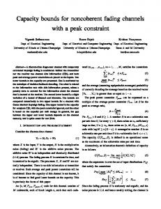
where fZi (q) is the probability density function of Zi . Figure 2 shows the analytical and simulated probability density function of maxima for signal-to-noise-ratio (SNR) of 15 dB, roll-off factor of the SRC filter α = 0.6, number of samples per symbol N = 100 with a contribution of L = 300 symbols to the estimator. Figure 2 demonstrates that the simulated probability density function of maxima closely match the analytical probability density function.

JOURNAL OF COMMUNICATIONS, VOL. 4, NO. 6, JULY 2009

407

analytical results closely match with the simulated pdf.

1 Simulated pdf of maxima Analytical pdf of maxima

0.9 0.8

Simulated pdf of τ Analytical pmf of τ

0.6

0.12

0.5 0.4

Probability density of τ

pdf of maxima (fQ(q))

0.14 0.7

Eb/N0 = 15 dB

0.3 0.2 0.1 0 220

221

222

223

224 225 Maxima (q)

226

227

228

229

0.1

0.08

0.06

0.04

0.02

Figure 2. Probability Density Function of Maxima 0 0

B. Probability Distribution of the Timing Estimator In order to determine the probability of bit error in the receiver, the distribution of the timing estimate errors must be taken into account. When using feedback techniques, the probability density function (pdf) of the timing error may be modelled using a Tichanov pdf [6]. Alternatively if the signal to noise ratio (SNR) is greater than the inverse of twice the variance of the timing offset, a Gaussian pdf may be used [10]. However, in our case the timing estimates relate to the maximum energy of the signal. The instant of time at maximum signal energy is the estimate. Considering this, we find an expression for the probability mass function of timing estimates. The analytical expression is then compared with the simulated distribution. Let N = 2N 0 + 1, and consider the two vectors, τ = [τ−N 0 , .., τ0 , .., τk0 .., τN 0 ] and Γ1 (k 0 , τ ) = [Γ1 (−N 0 ), .., Γ1 (0), .., Γ1 (k 0 ), .., Γ1 (N 0 )] with q = max(Γ1 (k 0 , τ )). Then, when the particular time instance τk0 is chosen as the timing estimate τˆ, that is τˆ = τk0 , the probability can be written as P (ˆ τ = τk0 ) = P (q = Γ1 (k 0 , τ )) = P (q > Γ1 (−N 0 ), .., q = Γ1 (k 0 ).., q > Γ1 (N 0 )) 0

= fΓ1 (k0 ) (q)

N Y

FΓ1 (j) (q)

(22)

j=−N 0 ,j6=k0

where, fΓ1 (k0 ) (q) and FΓ1 (j) (q) are the probability density function and cumulative distribution function of Γ1 (k 0 ) respectively. The expression for the probability mass function (pmf) for the timing estimates is given by, ½ P (ˆ τ = τ ); τ ∈ [τ−N 0 , .., τk0 .., τN 0 ] fτˆ (τ ) = (23) 0; τ 6∈ [τ−N 0 , .., τk0 .., τN 0 ]. Figure 3 shows the analytical probability mass function and the simulated probability density function for the timing estimates when SNR is 10 dB, roll-off factor α = 0.6, samples per symbol N = 100, and L = 300 symbols used for timing estimates. It is seen that the © 2009 ACADEMY PUBLISHER

20

40

τ/Ts

60

80

100

Figure 3. Analytical and simulated probability distribution function for timing estimates.

V. P ERFORMANCE OF THE E STIMATOR The statistics of the estimates are the key elements in determining the performances of the symbol timing recovery method. If the estimates are biased, the resulting sampling location selected by the symbol timing estimator will be biased from the true optimum and performance will suffer. Similarly, if the estimates have a high variance, the variance of the selected sampling location will also be high. Clearly it is desirable to keep the variance of the estimates as low as possible. The performance bounds for the symbol timing estimator are the CRB and MCRB. We evaluate the performance of the estimator finding bit error probability with matched filter detection and measuring variance of the estimator. Bit error probability is compared to the theoretical bit error probability for AWGN and variance is compared with the lower bounds CRB and MCRB. Figure 4 shows the bit error performance for the NDA-NML estimator in an AWGN channel when roll-off factor α = 0.6 in both transmitter and receiver, N = 20 samples per symbol, and L = 100 symbols used for timing estimates; with the further assumption that there is negligible inter-symbol interference. NDA-NML estimator exhibits good bit error performance compared with theoretical BER of AWGN. A. Cramer Rao Bound (CRB) We consider the additive noise only case to derive the CRB here, assuming that the received continuous waveform as given in (3) has complex envelope given by z(t) = s(t) + n(t) (24) which is observed over an interval T . s(t) is the information bearing signal and n(t) represents complex-valued

408

JOURNAL OF COMMUNICATIONS, VOL. 4, NO. 6, JULY 2009

with respect to time t evaluated at t = 0. For a raised cosine channel when the signal energy normalized to 00 unity, g0 (0) is given by [13] ´ ³ π2 00 + α2 (π 2 − 8) (28) g0 (0) = − 3 where α is the roll-off factor of the raised cosine filter.

0

10

−1

10

−2

BER

10

−3

10

α = 0.6 L = 100

B. Modified Cramer Rao Bound (MCRB)

−4

10

−5

10

ˆ The MCRB by [14] to the variance of λ(z) − λ is the following

Simulation with RCF and NML AWGN Theory

M CRB(λ) =

−6

10

−2

0

2

4 Eb/N0 (dB)

6

Ez,u

8

Figure 4. Bit error performance: NDA-NML estimator in an AWGN channel.

additive white Gaussian noise with two-sided power spectral density. Some of the parameters are unknown, such as the carrier phase θ, the symbol epoch τ , the carrier frequency error ν, etc. In order to estimate of a single element of {θ, τ, ν}, denoted by λ, which is assumed to be deterministic (nonrandom), all the other parameters, including the data, are collected in a random vector u having a known probability density function p(u) which does not depend on λ. If ˆ λ(z) is any unbiased estimator of λ, a lower bound to the ˆ variance of the error λ(z)−λ is given by the Cramer-Rao formula [11] CRB(λ) =

nh Ez

1 ∂ ln p(z|λ) ∂λ

i2 o

nh

(25)

where Ez denotes statistical expectation with respect to the subscripted variable, and p(z|λ) is the probability density function of z for a given λ. To compute CRB(λ) we need p(z|λ) which, in principle, can be obtained from the integral Z ∞ p(z|λ) = p(z|u, λ)p(u)du (26)

1 ∂ ln p(z|u,λ) ∂λ

i2 o .

(29)

This bound is found by [14] observing that n o n o ˆ ˆ Ez,u [λ(z) − λ]2 = Eu Ez|u [(λ(z) − λ)2 ] ) ( 1 ≥ Eu ´2 i h³ Ez|u ∂ ln p(z|u,λ) ∂λ 1

(

≥

h³

Eu Ez|u =

nh Ez,u

∂ ln p(z|u,λ) ∂λ

1 ∂ ln p(z|u,λ) ∂λ

i2 o

) ´2 i

(30)

where the first inequality derives from application of the ˆ CRB to the estimator λ(r) for a fixed u, while the second is true in view of Jensen’s inequality and the convexity of the function x1 for x > 0. In spite of having same structure of CRB and MCRB, MCRB is much easier to use. For Gaussian Channel, the probability density for (29) is a well-known exponential function whose argument is a quadratic form in the difference between z and the signal s. Thus the logarithm of p(z|u, λ) equals this quadratic form and the expectation in (29) is readily derived. The MCRB of symbol epoch (τ ) by [5] is given by 1

M CRB(τ ) =

8π 2 Lξ

−∞

T2 Es /N0

(31)

where p(z|u, λ), the conditional probability density function of r given u and λ is easily available, at least for additive Gaussian channels. Unfortunately, in most cases of practical interest, the computation of (25) is impossible because either the integration in (26) cannot be carried out analytically or the expectation in (25) poses insuperable obstacles. Using the general form of CRB given by [12], the CRB for timing estimates for AWGN channel can be written as: # " ³τ ´ 2Eb 00 2 (27) g (0)LT = − CRB N0 0 T

where L is the number of symbol intervals on which receiver bases its timing estimate on the observation on the received signal, T is the symbol interval, Es is the energy of one symbol waveform and ξ is an adimensional coefficient depending on the shape of g0 (t): R∞ 2 2 T f |G(f )|2 df R∞ . (32) ξ = −∞ |G(f )|2 df −∞

where L represents the number of symbols used to make the estimate of the timing offset, T is the symbol period, 00 g (0) is the second derivative of the pulse shaping filter

where

© 2009 ACADEMY PUBLISHER

MCRB for a normalized τ is given by [15] where τ is between 0 and 1. The MRCB is 1 (33) M CRB(τ ) ≥ 2LΓ(Es /N0 ) Γ=

T2 Es

Z 0

T

gd2 (t)dt

(34)

JOURNAL OF COMMUNICATIONS, VOL. 4, NO. 6, JULY 2009

where gd (t) denote the time derivative of g0 (t), Es is the 2 symbol energy. For a raised cosine pulse Γ = 4π3 . Figure 5 shows variance of the NDA-NML estimator with respect to CRB and MCRB when roll-off factor α = 0.6 and N = 40 samples per symbol. It is demonstrated in [14] that MCRB is generally lower than (at most equal) to the true CRB. The simulation result exhibits that the CRB is always greater than MCRB and the variance of the estimator is greater than CRB and MCRB as well. The variance of the estimator decreases as the number of symbols contributed for the timing estimation increases. With the increasing number of symbols used for estimation, the performance of the estimator improves in terms of variance. If the number of symbols contributed for the estimation is significantly small, then the performance of the estimator will be degraded. It is easy to implement the NDA-NML estimator and the complexity is low as well. −1

10

Variance of timing estimates

−2

10

−3

10

−4

10

−5

10

−6

10

NML L=100 CRB L=100 MCRB L=100 NML L=200 CRB L=200 MCRB L=200 NML L=50 CRB L=50 MCRB L=50

−5

0

5

well known that the envelope of the sum of two quadrature Gaussian noise signals obeys a Rayleigh distribution [16– 18]. The Rayleigh distribution has a probability density function given by ( ¢ ¡ r2 r 0≤r≤∞ − 2σ 2 , 2 exp σh h (35) f (r) = 0, r 0 is the shape parameter which defines the severity of fading and a > 0 is the scale parameter of the distribution. Smaller value of shape parameter indicates more severity of fading. In the special case when b = 1, the Weibull distribution becomes an exponential distribution; when b = 2, the Weibull distribution specializes to a Rayleigh distribution. For simulation purpose, for generating Weibull distributed random variates, at first a random variate U drawn from the uniform distribution in the interval (0, 1) is generated. Then the random variate hW = a(− ln(U ))1/b is generated which has a Weibull distribution with parameters b and a. hW is used as the fading amplitude for Weibull fading. While generating U , zero values are excluded to avoid natural log of zero. Sampled received signal experiencing Weibull fading can be expressed by (5) where the fading process h(kTs ) is the Weibull distributed fading amplitude hW . BER when the timing estimator operates under Weibull fading channel is demonstrated in Figure 7 for various Weibull shape parameters for roll-off factor α = 0.6, N = 15 samples per symbol and L = 100 symbols used for the timing estimates. With increasing value of shape parameter, the BER performance improves.

© 2009 ACADEMY PUBLISHER

The log-normal distribution has traditionally been used to describe the noticeable change in mean signal level (slow fading) experienced by a mobile receiver moving over long distances within a multipath environment. Rapid signal fluctuations about the local mean may also be observed over much shorter distances, typically in the order of tens of wavelengths [30]. Log-normal smallscale fading has been reported for some radio channels, particularly in indoor environments [31–33]. Recently, extensive effort has been directed at characterization of the propagation channels that involve the human body. Research into on-body channels [32], where communications is across the surface of human body and off-body [33], where a bodyworn radio device is communicating with remote terminal, have both reported small-scale fading which has followed the log-normal distribution. A statistical characterization of the narrowband dynamic human on-body area channel was presented in [34] demonstrating that log-normal distribution provides a good fitting model, particularly when the subject’s body is moving. The log-normal probability density function p(r) for an envelope R may be expressed as ³ −[log(r) − µ ]2 ´ 1 L √ exp (40) pR (r) = 2 2σL rσL 2π for r > 0, where µL and σL are the log-mean and logstandard deviation and both of which are found from log[p(r)]. For our simulation purpose, at first a random variate S is generated which is drawn from the normal distribution with 0 mean and 1 standard deviation and then the variate hL = exp(µ + σS) is generated which has a lognormal distribution with parameters log-mean µL and logstandard deviation σL . Sampled received signal experiencing log-normal fading can be expressed by (5) where the fading process h(kTs ) is the log-normal distributed fading

JOURNAL OF COMMUNICATIONS, VOL. 4, NO. 6, JULY 2009

amplitude hL . Figure 8 exhibits the BER performance for the timing estimator operating under log-normal fading when roll-off factor α = 0.6, N = 15 samples per symbol, and L = 100 symbols used for timing estimates. This performance is for the on-body wireless transmission scenarios where there is log-normal fading. Performance decreases significantly with the increasing of standard deviation. Small change of mean of the log-normal distribution does not have significant effect on the performance.

411

comparison of the Rayleigh fading, Weibull fading and log-normal fading, in Figure 9. It is clear in Figure 9 that the estimator performs similarly considering these fading conditions. Characterizations of these three types of fading are reasonably different with respect to the application of the NDA-NML estimator. 0

10

Rayleigh fading Weibull fading Log−normal fading 0

−1

10

BER

10

−1

10

−2

10 −2

BER

10

µL = 0, σL = 0.75 −3

10

µL = 0, σL = 0.50 µL = 0, σL = 0.25

−3

10

µ = 2, σ = 0.75 L

−4

10

L

µ = 2, σ = 0.50 L

L

−2

0

0

2 Eb/N0 (dB)

4

6

8

Figure 9. Bit error performance of NDA-NML estimator under various fading.

−5

10

−2

L

µ = 2, σ = 0.25 L

−4

2

4

6

8

E /N (dB) b

0

Figure 8. Bit error performance of NDA-NML estimator under lognormal fading.

Figure 9 shows the BER performance for three kinds of fading stated before. In every case, roll-off factor α = 0.6, N = 25 samples per symbol, and L = 300 symbols for timing estimation are considered. In Figure 9, standard Rayleigh fading with fading amplitudes that are based on complex fading coefficients with mean 0 and variance 1 is considered. For the Weibull fading channel, the scale parameter a = 1 and shape parameter b = 1.5 are used. For the log-normal fading channel, log-mean µL = 0 and log-standard deviation σL = 0.75 are used. The parameters for each of three different types of fading are appropriate to typical small-scale fading scenarios. From the Figure 9, it is demonstrated that BER performance for the Rayleigh fading channel is better than that of the Weibull fading and the log-normal fading channel and the performance of the Weibull fading channel is better than that of the log-normal fading channel. The performance will vary depending on the value of fading parameters. The estimator performs better for Rayleigh fading than Weibull fading, because of the more fading severity of the Weibull fading. For the Weibull fading, 1.5 is used for shape parameter which is compared with a shape parameter of 2 corresponding to Rayleigh fading, which indicates more severity of the Weibull fading scenario. The estimator performs better for Rayleigh fading than that of log-normal fading because of the higher variance used in Figure 9 of the log-normal fading. The estimator is shown to be robust to a change of fading conditions in © 2009 ACADEMY PUBLISHER

VII. C ONCLUSION Statistical performance of a NDA-NML timing estimator was presented. Several interesting aspects of the timing estimator were revealed examining the statistical distribution of the estimator. The expression for maxima and expression for the probability mass function of the timing estimates were derived and compared with the simulated density function. The performance of the estimator was assessed considering the BER, and the error variance was compared to the CRB and MCRB for AWGN channel. Finally, performance of the estimator was studied when operating under different fading scenarios with different characterizations by calculating the BER and the estimator was shown to be robust to change of fading conditions. ACKNOWLEDGMENT The authors would like to thank National Information and Communication Technology (ICT) Australia (NICTA). NICTA is funded by the Australian Government as represented by the Department of Broadband, Communications and the Digital Economy and the Australian Research Council through the ICT Centre of Excellence program. R EFERENCES [1] K. H. Mueller and M. Muller, “Timing Recovery in Digital Synchronous Data Receiver,” IEEE Trans. Communications, vol. 24, no. 5, pp. 516–531, May 1976. [2] F. M. Gardner, “Interpolation in Digital Modems-Part I: Fundamentals,” IEEE Trans. Communications, vol. 41, no. 3, pp. 501–507, Mar. 1993.

412

[3] ——, “Interpolation in Digital Modems-Part II: Implementation and Performance,” IEEE Trans. Communications, vol. 41, no. 6, pp. 998–1007, June 1993. [4] S. Kandeepan and S. Reisenfeld, “DSP based symbol timing estimation techniques,” in Proceedings of the IEEE ICICS-PCM’03, Dec. 2003, pp. 568–572. [5] U. Mengali and A. N. D’Andrea, Synchronization Techniques for Digital Receivers. New York and London: Plenum Press, 1997. [6] W. C. Lindsley and M. K. Simon, Telecommunication Systems Engineering. New Jersey: Prentice Hall, 1973. [7] K. Bucket and M. Moeneclaey, “Timing Jitter Sensitivity Comparison of Narrowband M-PSK and Bandlimited DS/SS M-PSK Signals,” IEEE Trans. Communications, vol. 1, no. 3, pp. 453–457, May 1993. [8] W. K. M. Ahmed and P. J. McLane, “On the Error Exponent for Memoryless Flat Fading Channels with ChannelState-Information Feedback,” IEEE Communications Letters, vol. 3, no. 2, pp. 49–51, Feb. 1999. [9] T. Ghirmai, “Data Detection and Fixed Symbol-Timing Estimation in Flat Fading Channels,” in Proceedings of the IEEE CISS, Mar. 2007, pp. 49–51. [10] J. J. Stiffler, Theory of Synchronous Communications. Prentice Hall, 1971. [11] S. M. Kay, Fundamentals of Statistical Signal Processing: Estimation Theory. Prentice Hall PTR, 1993. [12] T. Jesupret, M. Moeneclaey, and G. Ascheid, “Digital Demodulator Synchronisation-Performance Analysis,” European Space Agency Rep. ESTEC Contact No. 8437/89/NL/RE, June 1991. [13] C. N. Georghiades and M. Moenecleay, “Sequence Estimation and Synchronization from Nonsynchronised Samples,” IEEE Trans. Inform. Theory, vol. 37, pp. 1649–1657, Nov. 1991. [14] A. D’Andrea, U. Mengali, and R. Reggiannini, “The Modified Cramer Rao Bound and Its Application to Synchronization Problems,” IEEE Trans. Communications, vol. 2/3/4, pp. 1391–1399, Feb./Mar./Apr. 1994. [15] S. C. White and N. C. Beaulieu, “Improved Bounds for Timing Estimation Jitter,” in Proceedings of the IEEE GLOBECOM’90, Dec. 1990, pp. 609–616. [16] J. P. E. Biglieri and S. Shamai, “Fading Channels: Information Theoretic and Communications Aspects,” IEEE Trans. Inform. Theory, vol. 44, no. 6, pp. 2619–2692, Oct. 1998. [17] C. Loo and N. Secord, “Computer Models for Fading Channels with Applications to Digital Transmission,” IEEE Trans. Vehicular Tech., vol. 40, no. 4, pp. 700–707, Nov. 1991. [18] T. S. Rappaport, Wireless Communications, Principles and Practice. Prentice Hall, 1996. [19] H. Hashemi, “The Indoor Radio Propagation Channel,” in Proceedings of the IEEE, vol. 81, July 1993, pp. 943–968. [20] R. K. Mallik, “On Multivariate Rayleigh and Exponentials Distributions,” IEEE Trans. Inform. Theory, vol. 49, no. 6, pp. 1499–1515, June 2003. [21] N. H. Shepherd, “Radio Wave Loss Deviation and Shadow Loss at 900 MHz,” IEEE Trans. Vehicular Tech., vol. 26, pp. 309–313, Nov. 1977. [22] N. S. Adawi, “Coverage Prediction for Mobile Radio Systems Operating in the 800/900 MHz Frequency Range,” IEEE Trans. Vehicular Tech., vol. 37, pp. 3–72, Feb. 1988. [23] A. Babich and G. Lombardi, “Statistical Analysis and Characterization of the Indoor Propagation Channel,” IEEE Trans. Communications, vol. 48, pp. 455–464, Mar. 2000. [24] J. Cheng, C. Tellumbura, and N. C. Beaulieu, “Performance Analysis of Digital Modulations on Weibull Fading Channels,” in Proceedings of the IEEE Vehucular Technology Conference, vol. 1, Oct. 2003, pp. 236–240. [25] G. Tzeremes and C. G. Christodoulou, “Use of Weibull Distributions for Describing Outdoor Multipath Fading,” in

© 2009 ACADEMY PUBLISHER

JOURNAL OF COMMUNICATIONS, VOL. 4, NO. 6, JULY 2009

[26]

[27]

[28]

[29]

[30] [31]

[32]

[33]

[34]

Proceedings of the International Symposium on Antennas and Propagation Society, vol. 1, 2002, pp. 232–235. N. C. Sagias, D. A. Zogas, G. K. Karagiannidis, and G. S. Tombras, “Channel Capacity and Second Order Statistics in Weibull Fading,” IEEE Communications Letters, vol. 8, pp. 377–379, June 2004. M. H. Ismail and M. M. Matalgah, “Performance of Dual Maximal Ratio Combining Diversity in Non-identical Correlated Weibull Fading Channels using Pade Approximation,” IEEE Trans. Communications, vol. 54, no. 3, pp. 397–402, Mar. 2006. W. Xie and S. Liu, “Outage Probability Analysis of Dualbrach Transmit-selective System Over Correlated Modified Weibull Fading Channels,” in Proceedings of the IEEE International Conference on Communications, Cicuits and Systems, vol. 2, June 2006, pp. 659–663. M. H. Ismail and M. M. Matalgah, “BER Analysis of BPSK Modulation Over the Weibull Fading Channels with CCI,” in Proceedings of the IEEE Vehicular Technology Conference, Sept. 2006, pp. 1–5. W. C. Jakes, Microwave Mobile Communications. New York: Wiley, 1974. R. Gonesh and K. Pahlavan, “Statistics of Short Time Variations of Indoor Radio Propagation,” in Proceedings of the International Conference on Communications, June 1991, pp. 1–5. A. Fort, C. Desset, P. D. Doncket, P. Wanbacq, and L. V. Biesen, “An Ultra-wideband Body Area Propagation Channel Model-from Statistics to Implementation,” IEEE Trans. Microw. Theory Tech., vol. 54, pp. 1820–1826, 2006. S. L. Cotton and W. G. Scanlon, “Indoor Channel Characterisation for a Wearable Antenna Array at 868 MHz,” in Proceedings of the IEEE Wireless Communication and Networking Conference, Apr. 2006, pp. 1783–1788. D. Smith, L. Hanlen, D. Miniutti, and J. Zhang, “Statistical Characterization of the Dynamic Narrowband Body Area Channel,” in Proceedings of the International Symposium on Applied Sciences on Biomedical and Communication Technologies, Oct. 2008, pp. 1–5.

Md. Tofazzal Hossain is currently a PhD candidate in Information Engineering specifically in the areas of wireless communications at Australian National University, Canberra, ACT, Australia. He was born in Mymensingh, Bangladesh in 1984. He received his Bachelor of Science in Computer Science and Engineering from Khulna University of Engineering and Technology, Khulna, Bangladesh in 2005. He was awarded Prime Minister Gold Medal and University Gold Medal for his academic Excellence. He received his Masters of Information and Communication Technology from Australian National University in 2007. He was awarded National Information and Communication Technology (ICT) Australia (NICTA) Scholarship for his Masters and PhD. He was a lecturer of the department of Computer Science and Engineering at the Khulna University of Engineering and Technology, Khulna, Bangladesh, 2005-2007. His research interests include body-area communications, cooperative communications, low power communications and synchronization techniques for modern digital receivers.

Sithamparanathan Kandeepan was born in Colombo in 1975, he did his undergraduate level of studies in Colombo by completing the Engineering Council (UK) examinations majoring in communications and control systems engineering, he then went on to complete his Masters in Engineering (Telecommu-

JOURNAL OF COMMUNICATIONS, VOL. 4, NO. 6, JULY 2009

nications) in 2000, and his PhD in Electrical Engineering in 2003, both at the University of Technology, Sydney. Kandeepan currently is a senior researcher with the Create-Net International Research Centre in Trento, Italy working on various Industrial and European Union funded projects on applied and fundamental research in the areas of wireless, satellite and cognitive radio communications. In the past (2000 to 2004), he worked with the Cooperative Research Centre for Satellite Systems (CRCSS) on the FedSat micro satellite project in Sydney, whilst with the CRCSS he won the Earth Station Satellite Fellow award at the University of Technology, Sydney and from 2004 to 2008 he was with the National ICT Australia (NICTA) in Canberra as a Researcher working on wireless signal processing. Kandeepan a member of the IEEE since 2001.

David Smith was born in 1974. He received the B.E. degree in electrical engineering from the University of N.S.W. Australia in 1997, while studying toward this degree he was on a CO-OP scholarship. He obtained an M.E. (research) degree in 2001 and a Ph.D. in 2004 both from the University of Technology, Sydney (UTS) and both in telecommunication engineering, specifically in the area of wireless communications. He has also had a variety of industry experience in telecommunications planning; radio frequency, optoelectronic and electronic communications design and integration. He is currently a researcher at National ICT Australia (NICTA) and is an adjunct research fellow with the Australian National University, both since 2004. His research interests include: MIMO systems; coherent and non-coherent space-time coding; body-area communications; radio propagation and electromagnetic modelling; and antenna design.

© 2009 ACADEMY PUBLISHER

413