TinyIPFIX: An Efficient Application Protocol For Data Exchange In ...

TinyIPFIX: An Efficient Application Protocol For Data Exchange In Cyber Physical SystemsI Corinna Schmitt, Thomas Kothmayr, Benjamin Ertl, Wen Hu, Lothar Braun, Georg Carle Department for Informatics, Communication Systems Group, University of Zurich, Switzerland, [email protected] Department of Computer Science, Technische Universit¨ at M¨ unchen, Germany, [email protected], {carle, braun}@net.in.tum.de Institute for Telecommunication Systems, Chair for Next Generation Networks, Technische Universit¨ at Berlin, Germany, [email protected] CSIRO, Brisbane, Australia, [email protected]

Abstract Wireless sensor networks (WSNs) as a central part of cyber-physical systems are gaining commercial momentum in many areas, including building monitoring and intelligent home automation. Users wish to successively deploy hardware from different vendors. Interoperability is taken for granted by the customers who want to avoid the need for exhaustive configuration and set-up. Therefore, the need for an interoperable and efficient application layer protocol for machine-tomachine communication in and across the boundaries of WSNs arises. We address these issues with our implementation of TinyIPFIX, an adaption of the IP Flow Information Export (IPFIX) protocol. Throughout the paper we show how to leverage TinyIPFIX in the context of an office scenario and we discuss how the protocol may be applied to other significant WSN deployments presented in literature over the past few years. This article additionally shows how to improve the functionality of TinyIPFIX by adding both syntactic and semantic aggregation functionality to the established system. Finally, we evaluate the performance of TinyIPFIX in a large test bed with over 40 motes running TinyOS and analyze TinyIPFIX’s system performance in comparison with previous approaches. Keywords: wireless sensor networks; TinyIPFIX; aggregation; efficient data format, cyber-physical system.

1. Introduction The Internet of Things (IoT) is seeing rapid adaption across many industries. For example, Cisco Systems is predicting a growth from 369 million machine-to-machine (M2M) modules in 2012 to 1.7 billion M2M modules globally in 2017 [3] - and these figures are only for mobile M2M devices that connect via cellular networks. Arguably, the number of devices connecting via local wireless networks is even higher. Because the IoT has a plethora of different usage scenarios [4], it also covers a wide range of device I Part of this work was published in Proceedings of the 7th European Conference on Wireless Sensor Networks (EWSN) [1] and was mostly done when Corinna Schmitt and Benjamin Ertl were with Technische Universit¨ at M¨ unchen [2]. The extensions to the EWSN article include: First, an in-depth analysis on how to apply TinyIPFIX for a wide range of sensor network deployments. Secondly we demonstrate in-network aggregation support under TinyIPFIX, which includes data and message aggregation, as well as individual and direct configuration of the aggregation functionality on aggregator nodes. Third, an extensive analysis and system level evaluation of TinyIPFIX‘s transmission efficiency and resource consumption is presented along with a comprehensive comparison with other approaches. Compared to the original paper, there are significant modifications in Sections 3.4, 4, and 5.

Preprint submitted to Computer Communications

classes from powerful smartphones on the high end to devices that are highly constrained in memory, energy supply and computing capacity. The focus of this paper lies in delivering an efficient application protocol for machine-to-machine communication in a cyber-physical system. Our target device classes are the constrained devices (motes) found in wireless sensor networks (WSNs), which often form a key component of a CPS. One common application area can be found in the field of building automation, meaning the autonomic monitoring and control of environmental conditions in residential and commercial buildings for improved comfort, as well as a reduced energy usage and carbon footprint. Wireless sensors are deployed to monitor key values, such as room temperature or brightness, in different locations. They transmit the data to a control and management system, which analyses the measurements and reacts on the results, e.g. turning on/off heating or lights. Not only the devices themselves are constrained in this scenario. The low power wireless network over which they communicate also imposes severe limits on throughput and message size. Any application protocol used in this scenario must be efficient in its use of network, computational and energy May 21, 2014

and Type IDs have been allocated globally unique, a public repository for this semantic data, presented as XML markup, becomes feasible. We will give an example for such a markup in Section 5.4.

resources. However, it should still be comfortable to use for the system developer as well as complete and generic enough to allow easy deployment by the end user. Web services are a well-known approach to M2M communication, but directly adapting the techniques from traditional computing are not feasible in constrained networks because they rely on verbose XML formats to exchange messages. For example, it takes up to 442 bytes to get a temperature value encapsulated with SOAP 1.2 [5]. This is often addressed through compression of the XML data [6] or by directly encoding the XML message in a binary format [7]. HTTP itself is also considered too resource intensive for constrained networks and alternatives like the Constrained Application Protocol (CoAP) [8] have been developed. The related work is discussed in Section 2 in more detail. While suited to the domain of constrained networks, CoAP also introduces additional implementation complexity that might not be needed in all usage scenarios of WSNs. For example, a wireless thermometer that periodically reports to an automation server with a direct user interface is duplicating functionality that is available by accessing the data on the data sink it is reporting to. Our approach focuses on the core functionality of stationary Wireless Sensor Networks: Periodic reporting of sensor data to a data sink with low network, memory and computational overhead while still enabling easy integration of diverse sensor hardware on motes from different vendors with minimal configuration and maintenance overhead. The approach is centered around TinyIPFIX, a lightweight adaption of the IP Flow Information Export (IPFIX) protocol [9] for WSNs. Section 3 presents a brief characterization of the TinyIPFIX protocol and discusses its characteristics focusing on the constrains of wireless sensor nodes. In general, the design space for an application protocol to achieve tight integration of a WSN into a CPS consists of four areas:

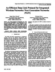
Resource Efficiency: The resources of sensor nodes are limited in terms of power, memory space and computational capacities. We evaluate TinyIPFIX with regard to its memory requirements and energy consumption. Additionally, we implemented the TinyIPFIX-Aggregation protocol, which offers in-network aggregation mechanisms for data pre-processing. By leveraging in-network aggregation additional energy savings can be achieved through transmission reduction. Syndication: The benefits of using IPv6 in sensor networks were detailed in previous work [10]. We choose to send TinyIPFIX packets via the BLIP [11] implementation of IPv6 and UDP, because it offers seamless integration into an existing IP-based network infrastructure. Scalability: In Section 5.1 we discuss the flexibility of TinyIPFIX by showing how it could have been leveraged in other significant deployments presented at IPSN or SenSys over the past few years. We present the results of numerous real world test runs of TinyIPFIX assuming an office scenario (see Figures 1 and 10) and in a large WSN deployment on the Harvard Sensor Network Testbed (Motelab) testbed [12]. Section 4 describes the integration of a TinyIPFIX based wireless sensor network into a cyber-physical system used for building automation. We evaluate the performance of the TinyIPFIX protocol concerning its hardware requirements and demonstrate the functionality of the whole system in Section 5 before concluding the paper in Section 6. 2. Related Work

Metrology: Sensor devices measure data, which has a specific format and must be represented accordingly. This representation should be general and universal, meaning that a protocol should be able to uniquely designate each measurement type across all WSN deployments. A measurement type is defined here as a reading from a specific model of a sensor, which carries information about the data type and its conversion to scientific units, rather than an abstract quantity such as “temperature”. In the case of TinyIPFIX the sensor measurement data is identified by an individual Type ID and Enterprise Number (EID), which are registered with the Internet Assigned Number Authority (IANA)1 . This ensures adaptability to other platforms or new measurement types. Since an IPFIX Template only carries syntactical meta data for the measurements sent in an IPFIX Data packet the semantics for that data still need to be supplied. If the Enterprise

Widespread adaption of traditional web services in constrained networks is stymied by HTTP’s verbosity. With the Constrained Application Protocol (CoAP) Shelby et al. introduced a lightweight, yet interoperable, alternative to HTTP that allows the adaption of the web service principle to constrained networks [8]. Compared to HTTP, CoAP’s main benefits are a reduced header size and no requirement for reliable message transport (i.e., CoAP only requires UDP and not TCP). Motes that have data to expose implement a CoAP server and expose their data offerings to the data consumers via a discovery service. Similar to HTTP, CoAP does not specify the actual format in which data is transported but supports different content encodings. Our approach, which is centered on IPFIX, is more comparable to a content encoding format in the context of CoAP. CoAP and IPFIX for sensor networks therefore have different concerns: While CoAP’s goal is to bring the full suite of features that is required for a weblike experience to constrained networks, we aim to offer a

1 http://www.iana.org

2

Server

WSN Infrastructure

TinyIPFIX Data Set Template ID Node ID Value 1 = Temp. 2 = Brightness

TinyIPFIX Metadata Repository

1

2

XML Metadata

Central

1 3

4

20Management Entity

0

00

5 Data collection

Aggregator Nodes: Node ID 0, 3, 6 Aggregation functionality mode 1 or mode 2

XML Parser

3

6

2 6

Central Management Entity

1 3 2 6

Sensor Nodes: Node ID 1, 2, 4, 5 Measurement functionality

Field Metadata

20 200 Field Metadata Metadata

200

TinyIPFIX Field

Data g essin proc

Cloud of Application

Wireless Communication (perhaps aggregated messages) Logical control communication Wired Communication

Figure 1: Abstract system architecture

In the field of in-network aggregation two main approaches exist today: (1) message aggregation and (2) data aggregation, which is also referred to as pre-processing in literature. The first approach concatenates two or more messages into a newly generated aggregate message without data pre-processing. The second approach means to evaluate the data transmitted from one sensor node to another one and to compute aggregates on this data, based on requested types of values and aggregate functions. The naive approach consists of performing these aggregates on the data sink. A better strategy is to perform innetwork aggregation on sensor nodes with more resources. In this paper we present an in-network aggregation technique called TinyIPFIX-Aggregation, which implements message and data aggregation features. The remainder of this section briefly compares our approach to TAG, AIDA, and SIA. Those three approaches are the most prominent examples in literature. In 2002 Madden et al. presented a Tiny AGregation (TAG) service for ad-hoc sensor networks [16]. This approach is based on in-network data pre-processing, because applications often depend more on data aggregations rather than raw sensor data. The underlying aggregation queries are formulated in a syntax that is similar to the well-known SQL. Przydatek et al. presented a security framework called Secure Information Aggregation (SIA) for wireless sensor networks in 2003 [17]. In SIA, sensor nodes transmit raw sensor data unsecured and employ secured computation of aggregates. The computation of secure aggregates consists of three parts: (1) data collection and aggregation, (2) commitment of the collected data by the aggregator, and (3) establishing a communication protocol with the data sink. One example for the data collection and aggregation part is the implementation of a spanning tree in the network. Other algorithms can also be adapted. One year later He et al. presented the AIDA implementation, which is an Adaptive Application-Independent Data Aggregation approach [18]. The AIDA component resides between the data link layer and network layer with no specific application dependent knowledge. The component includes an aggregation module, which combines messages into new frames of the AIDA protocol. Due to the

simple M2M application protocol with minimal implementation and network overhead that can be used where the full set of features offered by CoAP is not necessary or the implementation complexity cannot be afforded. A more direct comparison can be drawn between IPFIX and different content encoding formats used with CoAP, HTTP or standalone: XML is arguably the most well known format for transferring structured data in a human readable way. However, the clear text format of XML results in very large message sizes and slow processing times - even in the field of traditional computing. JSON is a more compact format to transfer structured, human readable data but it still cannot achieve the same level of message compactness as binary formats. A large amount of effort has been undertaken to reduce the size of XML documents while simultaneously improving their processing speed. Two representative approaches are Fast Infoset [13] and Efficient XML Interchange (EXI) [7]. Compared to Fast Infoset, EXI achieves a higher rate of compression because it is able to take the structure information provided by an XML schema into account. However, both the encoding and decoding party needs to process the matching schema to leverage the increased rate of compression. A schema-less mode is available in EXI as well. Compared to our approach XML offers the capability to transfer structured (nested, repeating, value constrained, variable length etc.) data whereas IPFIX as specified in RFC 5101 [14] and more recently in RFC 7011 [9] has no support for structured data types. Further extensions, especially RFC 6313 [15], can be applied to overcome this limitation. However, it is our observation that most structure data is used to describe the metadata surrounding a measurement value or to group multiple sensor measurements into one message. How IPFIX deals with this issue of metrology is discussed in Section 3.2. The separation of data into a Template message is comparable to a message containing an XML schema without which binary XML approaches struggle to reach IPFIX’s level of compactness (c.f. Section 5.2.2). Overall, the implementation complexity of IPFIX is significantly lower than with any approach using XML or a binary XML format.

3

independence from the application layer, the AIDA framework can provide aggregation mechanisms for a range of different applications. No data semantics are lost during the aggregation process. AIDA merely combines received messages in larger frames for a better utilization of the communication channel, and, therefore, does not reduce the amount of the transmitted bytes, but as a result of less packets the amount of control messages can be reduced when congestion in the network occurs. Another advantage is the dynamically controlled degree of aggregation (DoA) in accordance with changing traffic conditions.

Set ID

Length

Template ID

Field Count

Template Record Template Field ID: Node ID

ID: Time Stamp ID: Temperature ID: Brightness

Set ID = Template ID

Length

Data Record Data Length ID: Node ID

Enterprise Number

Data Length ID: Time Stamp Data Length ID: Temperature

Enterprise Number Enterprise Number

Data Length ID: Brightness

Enterprise Number

(A) Template Set

3

1233419825

20

200

4

1233419827

34

500

Data Field

(B) Data Set

Figure 2: Components of the IPFIX protocol showing decoding of the data.

3. TinyIPFIX Design

corresponding field in the Data Record (Figure 2 shows four template fields). The type is uniquely described by a tuple consisting of a Type ID (two bytes), a length statement (two bytes), and an Enterprise Number (four bytes) in a Template Field. The Type ID specifies the type of data while the Enterprise ID denotes the organization, which issued the Type ID. Sensor nodes act as Exporters and transmit their measurement data using IPFIX. When a sensor node boots up, it has to announce its Template Record before sending its measurement data to the Collector. This has to be done only once since a Collector buffers the Template Record to decode incoming Data Records. They do not have to contain anything but the measurement data as all meta information has been already sent in the Template Records. A short header containing the number of transmitted values and the referenced Template ID only accompanies Data Records. Several Data Records can be put into a single message. Section 4 characterizes the implementation of IPFIX for WSNs in detail. From this point on we mean TinyIPFIX if we use IPFIX in WSN context. The computation costs for creating a template are very cheap and the number and size of different templates and messages used in parallel bound the additional memory requirements of TinyIPFIX. Therefore, TinyIPFIX can be used on nodes with constrained resources when they limit themselves to a few templates of small size, which will be demonstrated by our implementation in Section 5.2.1. Multiple templates can be used if the nodes have more resources. They may also analyze the data directly instead of shifting this task to a server.

We start this Section by giving a short overview of the original IPFIX protocol [9] before showing how it can be applied to sensor networks. 3.1. IPFIX overview IPFIX was developed by the Internet Engineering Task Force (IETF) for transmitting flow information between different instances in the network [9]. Communication takes place between an Exporter and a Collector. IPFIX is specified as a PUSH-protocol with an Exporter periodically transmitting data to one or more Collectors. This makes IPFIX an attractive choice for WSNs, because they often rely heavily on Collection traffic. This traffic pattern means that information flows from many source nodes to only a few information sinks such as the gateway nodes. A template-based design is used to exchange measurement data while minimizing overhead. Measurement data is exchanged in Records. The protocol distinguishes, amongst others, between Template Records and Data Records as shown in Figure 2. Together with the corresponding header those messages form a Template Set or Data Set. A detailed description of the data exchange and special requirements for sensor measurements can be found in reference [1]. Data Records contain the measurement data while Template Records contain the meta information of Data Records. The meta information covers the semantics, data type, and length of the measurement data. An Exporter sends a Template Record to its Collector to announce the structure of the upcoming Data Records. This Template record is only required once but may be repeated periodically. The Collector for decoding incoming Data Records stores the Template Record. A Template ID, which is unique for every Exporter and the templates it uses, is assigned to every Template Record sent to a Collector. Further Data Records will reference this ID. As shown in Figure 2, each Template Record describes the encoding of the transmitted sensor measurement values in a Data Record. A Template Record may contain several Template Fields where a field corresponds to a measurement type, e.g. brightness or humidity. Each field in the Template Record describes the type and length of the

3.2. Metrology The Type ID and the Enterprise Number (EID) identify Sensor measurement data. As described in the introduction, each measurement of a sensor should be assigned a globally unique combination of Enterprise and Type ID. For example, the Sensirion SHT11 temperature and humidity sensor would be assigned two different combinations, e.g. Enterprise ID 12345 and Type ID 32768 for its temperature channel and Enterprise ID 12345 and Type ID 32769 for its humidity channel. A public repository would 4

by limiting the capabilities of IPFIX to those required in WSNs. The IPFIX packet length is limited to 1,024 bytes, which exceeds the maximum packet length defined by the IEEE 802.15.4 standard and, thus, requires packet fragmentation [20], which may be provided by the underlying network layer. For example, it is possible to send IPv6 messages of up to 1,280 bytes length with BLIP [11]. With header compression, only one set of templates or data is transmitted. Figure 4 shows the header of the aggressive approach where the SetID field is moved to the front of the header and shortened to four bits. It acts as a lookup field for the SetIDs and provides shortcuts to often used SetIDs [21]. The bits marked E1 and E2 control the presence of the extended SetID field and the length of the Sequence Number field respectively. Typical WSN installations are sending messages in intervals of multiple seconds or more. Therefore, the Sequence Number field has been shortened to one byte, which should cover a sufficiently long timespan. Since IPFIX packets are always transported via an underlying network protocol, which specifies the source of the packet, the Observation Domain can be equated with the source of an IPFIX packet and the field can be dropped from the header. The specification of a 32-bit time stamp in seconds would require time synchronization across the WSN and produce additional protocol overhead. Thus, the Export Time is dropped in TinyIPFIX. Applications requiring an exact time stamp for their measurements can define an according field in the template and send the measurement time stamp along with the sensor data in a data packet. By using the header compression technique the IPFIX Message Header (16 bytes) and the first Set Header (four bytes) can be reduced from in total 20 bytes to only three bytes.

allow an application that receives a template with an Enterprise and Type ID combination that it has not seen before to obtain the semantics of that measurement from the Internet. The semantic information includes what kind of data (temperature), the data type (16-bit integer), how to convert to a sensor independent format (formula to convert to ◦ C), and any other required information. This would allow flexible deployments of motes with different sensors, for example, if an existing deployment using Sensirion SHT11 sensors was augmented with several new nodes that use a Sensirion SHT15 instead, there would be no need for extensive reconfiguration within the WSN or the converter application if both use IPFIX to send their measurement data. Nodes can simply transmit the raw measurements without having to convert them into other formats via potentially complex formulas. The receiving application on a PC can convert both values to scientific units and combine the measurements based on semantic information obtained from the repository. An example is shown in Section 5.4. 3.3. Adaptation to WSNs Since IPFIX was designed for conventional networks for monitoring tasks [19], some extensions and changes have to be introduced to increase its efficiency in the context of WSNs. The implementation for WSNs is called TinyIPFIX. One of the problems when deploying IPFIX in sensor networks is the overhead introduced by the relatively large header, as shown in Figure 3. In order to address this issue, a header compression scheme was developed, which is part of the TinyIPFIX protocol. Apart from header compression, TinyIPFIX is fully compliant with the IPFIX protocol. TinyIPFIX template and data set contents are identical to those of standard IPFIX.

3.4. In-network aggregation 0

16

31

As mentioned at the beginning of the paper the resources are very limited for wireless sensor devices, which makes saving resources important. One technique for saving energy and computational capacities is in-network aggregation [22]. Aggregation is usually performed on aggregator motes, which have more resources and are located at selected positions within the network. The following two aggregation techniques are common and implemented in our TinyIPFIX-Aggregation framework:

IPFIX Message Header Version Number

Message Length Export Time Sequence Number Observation Domian

IPFIX Set Header Set ID

Set Length Message Payload

Figure 3: General structure of IPFIX headers [bits].

0 1

2

6

E1 E2 SetID Lookup Sequence Number

1. Message Aggregation (mode 1): Aggregation of several data messages in one packet

15

• Type A: Data Records refer same Template

Length

• Type B: Data Records refer different Templates

Ext. Sequence Number

Ext. SetID

2. Data Aggregation (mode 2): Data pre-processing within the transmission path to the gateway through aggregate functions

Figure 4: Header used by aggressive TinyIPFIX approach [bits].

The first aggregation type (mode 1) can easily be performed if the link layer MTU is big enough. In the case of TinyIPFIX we can split this case into two subclasses. In

Because the header size has large influence on the overall transmission efficiency of TinyIPFIX, we have chosen an aggressive approach to header compression [1]. It starts 5

briefly illustrated in Figure 6 [23]. In order to allow this data transfer, parsers and interfaces are required, which are partly implemented in AutHoNe and in the WSN. A brief description is presented in parts of Section 5.

case 1.A several Data Records, which refer to the same Template, are transmitted in one message as shown in Figure 2 where two Data Records are transmitted in one packet. The second possibility (1.B) is the combination of two different Data Records in one message, which refer to different Template Sets. In this case the combined Data Set must refer all needed Template Sets for decoding. An example is shown in Figure 5. Assuming Figure 1 setting and looking at the transmitted messages between the aggregator nodes (node ID = 3,6,0) towards the server, the number of transmissions is reduced by one.

Template ID = 1

Length

Data Record – Typ 1 Node ID Temperature

3

1233419825

20

200

Template ID = 2

Node ID Temperature

Time Stamp

Figure 6: Examplary information flow in AutHoNe.

Brightness

Length

Data Record – Typ 2

4.1. General design decisions on the WSN side The choice of UDP over IPv6 as network and transport protocols allows the simple integration of motes into the network. A mature implementation of UDP/IPv6 for sensor networks exists in BLIP [11]. Figure 7 shows the used network stack.

Time Stamp

4

1233419827

34

78

Humidity

Figure 5: Data Set for in-network aggregation of mode 1.B.

The second type of aggregation (mode 2) uses the aggregate functions f = max {a, b}, f = avg {a, b} and f = min {a, b}. The chosen aggregation function depends on the application and is applied to contemporary measurements rather than temporal series of measurements. For example, if only the maximum temperature in a room is relevant, as shown in Figure 1 in the upper room, we can use f = max {a, b}. In this case the number of transmitted messages to the gateway node (node ID = 0) can be reduced by one in total. As pointed out by Krishnamachar et al. [22], in-network aggregation leads to an increase in data latency, which depends on the performed aggregation mechanism.

Figure 7: Structure of network stack

A matching application level protocol, which would facilitate the aforementioned properties while introducing limited protocol overhead, was still needed. We decided to use TinyIPFIX for this purpose since it is highly flexible while maintaining high transmission efficiency through the separation of meta data and sensor measurements into different messages. The Enterprise / Type ID metrology described in Section 3.2 allows the user to add new motes with sensors that were not known during the initial deployment because the semantic data can be dynamically obtained, thereby fulfilling our requirement for easy configuration. Other protocols such as the XML based COAP [8] or the JSON based sMAP [24] also meet the aforementioned requirements. However we wanted a simpler protocol that introduces very little computational, message and implementation overhead. We decided in favor of TinyIPFIX, because it does not need to perform compression to achieve high transmission efficiency as shown in Section 5.2.2.

4. An end-to-end cyber-physical system implementation In this section we show the design and implementation of a 6LoWPAN/TinyIPFIX based end-to-end cyberphysical system. It consists of the WSN infrastructure, the server, and a connection to the cloud. We use the term cloud to refer to a pool of applications and services, which require and access the collected data of the WSN as illustrated in Figure 1). For example, the project Autonomic Home Networking (AutHoNe) is a representative for a CPS in the cloud, which was tested in an office scenario. All components in AutHoNe communicate over IPv6 and require different information of all components. In the case of the WSN the AutHoNe infrastructure requests, among others temperature and humidity values in order to regulate the climate control automatically by comparing monitored data with preset thresholds for individual rooms as

4.2. Data preprocessing by TinyIPFIX-Aggregation Due to application requirements and limited resources of WSN components aggregation techniques are an attrac6

Performing Data Aggregation with f = maxTemp {node1, node2}

Template received

Data received

incoming packets

Data preprocessing

YES Data Aggregation (mode 2)

Message Aggregation (mode 1) Template received

Data received

NO

NO

Server

Template update

NO

Performing Message Aggregation

Template update Count +1

Count == DoA

NO

Figure 8: Testbed 1: Overview of aggregation features. Black marked messages are original IPFIX records transmitted by sensor nodes. Red marked messages are IPFIX records transmitted by aggregators as result of aggregation functionality.

YES

Data update

YES

Template Count +1

Data received

YES

YES makeTemplate()

NO

Data update

YES

Data Count +1

Data update Count +1

Data Count +1

makeDate()

Data update Count +1

Count == DoA

Count == DoA

YES

YES

NO

NO

NO

YES makeAggregateData()

Wait for incoming packets

tive addition to cyber-physical system similar to those presented in this paper. Our TinyIPFIX-Aggregation framework offers the user two modes of aggregation: (1) message aggregation and (2) data aggregation. Both techniques work with the TinyIPFIX message format as it is shown in the example of Figure 8. [25, 2] The functionality of the protocol for message aggregation (mode 1) is shown in the lower room in Figure 8. Sensor messages up to a certain amount are aggregated into newly generated appropriate messages. The number of message aggregated is referred to as the degree of aggregation (DoA), which depends on the aggregator’s available memory as well as the number of sensor nodes in range of the aggregator, the acceptable message delay and application constraints. In the message aggregation mode information about the source sensor node of template and data sets is essential for reconstructing the data and must not be lost during the aggregation process. We address this requirement in our message aggregation algorithm. It is shown in Figure 9 on the left side and consists of the following steps [25, 2]:

Figure 9: Decision tree for TinyIPFIX-Aggregation

be announced independently of whether or not the associated data sets have been received. 4. Transmit the aggregated data set: The aggregated data set is now transmitted. 5. Update buffered data sets: The updated data sets are assigned to their buffered template sets and send periodically after the degree of aggregation has been reached. The timespan for receiving new data information is generally shorter than the interval for receiving new template information. 6. Update buffered template sets: If the aggregator receives a new template definition the buffer for the template set is updated. As a result, the conditions for the aggregation of new incoming data sets change which requires the received data to be reallocated according to the updated template definitions. The upper room shown in Figure 8 is showing data aggregation (mode 2) in contrast to message aggregation (mode 1). Resulting messages transmitted by the aggregators are shorter than in normal message aggregation mode. The idea behind this implementation is that the aggregator computes aggregates on the received sensor readings from the sensor nodes by applying aggregate functions on specific values such as MIN, MAX or AVG, i.e. the aggregator performs semantic aggregation in mode 2 whereas only syntactic aggregation is performed in mode 1. Because bidirectional communication is provided, the aggregate functions and the sensor reading types can additionally be selected and changed during operation. Selecting the aggregate function and value type via UDP-Shell commands does this. The underlying algorithm for data aggregation consists of the following steps and is shown in Figure 9 on the right side [25, 2]:

1. Buffer template sets: Before data can be transmitted the IPFIX protocol requires the announcement of the related template. Those are buffered by the aggregator to a maximum amount, the degree of aggregation (DoA). 2. Buffer data sets: Incoming data sets are also buffered and allocated to the corresponding template sets stored in the step before. If the requested template set is unknown the data set is dropped because it cannot be interpreted. 3. Transmit the aggregated template set: If the maximum amount of buffered template sets is reached, the aggregator announces the upcoming data with the aggregated template set. The template can 7

• Syndication −→ Application use: We integrated a WSN performing TinyIPFIX in the home infrastructure management project AutHoNe [27]. The included components in AutHoNe can use the measured data for controlling purposes (e.g. climate control). By having an interchange format via XML, other applications are “portable” from a collection of similar sensors.

1. Transmit new template set: Since the data preprocessing aggregation is driven by user requests for specific sensor readings, and, therefore, the recipient of the aggregated data already has knowledge of the meaning of the expected data, the transmission of a new template by the aggregator can be omitted. 2. Buffer template set: The aggregator buffers all incoming template sets from the sensor nodes till the buffer limit or the degree of aggregation is reached. 3. Buffer data set: Incoming data sets are associated with the matching template sets, which have been received earlier. After reaching the buffer limit or degree of aggregation for the data sets, the selected aggregate function is performed on the stored data sets. 4. Compute the aggregation function: In order to compute the selected aggregate function, sensor readings have to be converted from the sensors’ encoding of the measurement to an universal format. The aggregator holds a lookup table for the data values announced by the according template set, with which it can identify the desired value type. It then computes the aggregate function on all buffered values of that type. 5. Transmit the aggregated data set: After computing the aggregate function, a newly generated data set for the demanded value type with the aggregated values is generated and transmitted to the next aggregator or gateway. Additional information on the aggregated value can also be transmitted in the data set, assuming that the recipient can decode the information properly.

5.1. Complete and general Due to the separation of measurement data and corresponding meta information in two different message types, the TinyIPFIX protocol is very flexible. A suiting Template Set can be defined for almost any application scenario and may be changed by the motes as needed. It must only be ensured that the modified Template Set is announced to the recipients of the Data Sets. An optional periodic rebroadcast of the Template helps to address the issue of unreliable communication protocols and also gives Collectors, which join the network at a later time, the possibility to parse the incoming sensor data. The TinyIPFIX protocol is also independent from the mote’s hardware. Little to no changes (e.g. only changing the sensor code or adapting the maximum size of IPFIX packets) are needed to use TinyIPFIX on other platforms supported by TinyOS. So far, TinyIPFIX has been successfully tested on the IRIS and TelosB platforms. So far we have focused on an office application scenario. In order to widen the scope we discuss how TinyIPFIX may be applied to some major deployments from IPSN/SenSys from the past few years. These deployments were chosen, because each of them differs in the way that they send data to the gateway nodes and, therefore, represent a wide spectrum of possible deployments. In the remainder of this section IPFIX describes the unaltered protocol while TinyIPFIX refers to the implementation with activated header compression (cf. Section 3.3). For optimization purposes the TinyIPFIX-Aggregation framework introduced in Section 4.2 is included in the upcoming evaluation. HydroWatch is a sensor network deployed to monitor the “life cycle of water as it progresses through a forest ecosystem” [28]. It is is based on the TMote-Sky, which is compatible with TelosB motes. It periodically samples the photo synthetically active radiation (Hamamatsu S1087) and the total solar radiation (Hamamatsu S108701), as well as temperature and humidity from a Sensirion SHT15. The encoding of these measurements in an IPFIXTemplate are straightforward since the data flow model (periodic, single measurements, no back channel) is very similar to our home networking environment. Therefore, TinyIPFIX could have been used in this scenario without any changes to the protocol. References [29], [30], and [31] described a similar data flow pattern.

5. Evaluation In this section we evaluate TinyIPFIX extensively using the following metrics: • Metrology −→ Completeness and Generality: We discuss how TinyIPFIX can be used in different application scenarios and for different kinds of transmitted data. • Resource Efficiency: We evaluate the resource (RAM and ROM) consumption of the TinyIPFIX protocol, as well as the transmission efficiency in comparison to a common Type-Length-Value approach. Additionally we evaluate its system performance in a large WSN. • Scalability −→ Practical Implementation: We show that TinyIPFIX is easy to program and present an example in TinyOS. The protocol can also be transferred to other operating systems if the implementation follows the description as published in reference [26].

8

The goal of the project PermaSense is to collect geophysical data via 15 nodes installed in an alpine environment [32]. It samples rock temperature and electrical resistance at four different depths per node, as well as the internal voltage, temperature and humidity inside the enclosure of each node. One interesting point arises for how to encode having more than one measurement of the same type in one IPFIX packet. The basic idea of IPFIX for WSNs is to assign the Enterprise and Type IDs based on the manufacturer and model of the sensors used. In this case, one would have to deviate from this principle by defining an Enterprise ID for the project and separate Type IDs for each of the sensors at different depths. The semantic information would have to be supplied via an indirection, as an automatic lookup in a public repository via the Enterprise / Type ID combination would not yield the correct response. Instead one would have to instruct the program that queries the repository not to use the combination specified in the IPFIX template but the Enterprise and Type ID that corresponds to the correct sensor. Another point of interest comes from the properties of the data flow. PermaSense transmits data periodically as single measurements when a link between the gateway node and the sensor node exists. When the link is broken, e.g. when the mote is covered in snow, measurement data is logged and transmitted in bulk when connectivity is reestablished. Assuming bulk transmission, filling the IPFIX data packet with data records until the maximum packet size allowed by the transmission protocol is reached, can increase the relative transmission efficiency of IPFIX. The system Lance collects seismological data [33]. As such, it samples data at high rates (100Hz or higher) and performs event detection on the motes to decide, which parts of the recorded data are of potential interest since it is not feasible to transmit all measurements. The gateway node requests the bulk transfer of the data based on a cost model. Other application areas with similar modes of operation include habitat and structural integrity monitoring.

5.2. Resource efficiency This section deals with evaluation of resource consumption of the TinyIPFIX implementation with aggregation support. It is important to focus on resource consumption for long life support of the WSN, because the used sensor nodes (IRIS and TelosB) are constrained in memory, computational, and energy capacity. 5.2.1. Embedded implementation We implemented TinyIPFIX on top of the BLIP IPv6 and UDP implementation, which comes as a part of TinyOS-2.1.12 . In order to put the memory usage in perspective, each major component is considered separately. Since they build upon each other, the memory consumption has been measured in an incremental fashion, starting with a basic scaffold for obtaining measurements and expanding upon that by adding BLIP and TinyIPFIX. The results are shown in Table 1, which shows a maximum RAM consumption of 6,889 bytes when using BLIP and setting the maximum TinyIPFIX package size to 1,024 bytes. The memory consumption of the TinyIPFIX component is only 57 bytes plus twice the maximum defined IPFIX packet size. The memory consumption on IRIS is similar to that on TelosB. Component Scaffold BLIP TinyIPFIX

Total

RAM

ROM

TinyIPFIX Packet packet

46 4,738 57 261 2,105 4,841 - 6,889

2,826 23,012 2,972 3,182 3,012 29,020

0 102 1,024 0 - 1,024

Table 1: Memory usage of BLIP and TinyIPFIX [bytes]

1 2 3 0 4 0 5 0 6 85 7 0 8 1234 9 23 10

There is only one point where plain TinyIPFIX is struggling to achieve the required functionality. Currently it does not support a back channel as would be needed for the gateway node to request event records from the motes. This limitation could be fixed by introducing another template type for instructions: each node announces an instruction template after boot, which is periodically retransmitted. Any entity that wants to give a command to a node sends an IPFIX data packet that is in compliance with the previously announced instruction template. How to assign the Enterprise and Type IDs still remains an issue. However, IPFIX is fundamentally a PUSH-protocol and, therefore, does not natively support pulling data. Transmission of binary data of variable length is supported by the IPFIX specification [14, 9], although our implementation does currently not support this feature.

Listing 1: XML content used for a Smart Energy Meter. We assume a total size of 9 bytes for the values (five 8-bit integer and two 16-bit integer).

2 http://www.tinyos.net

9

Encoding XML EXIficient Binary XML FastInfoset IPFIX TinyIPFIX TLV 28 TLV 248

Listing 1

Listing 2

409B 13B (3%) 210B (51%) 200B (49%) 31B (8%) 13B (3%) 16B (4%) 51B (12%)

300B 57B (19%) 117B (59%) 185B (62%) 34B (11%) 16B (5%) 16B (5%) 40B (13%)

very high end-to-end data usable rates, e.g., approximately 97%, in a large multiple hop sensor network testbed). As can be seen in Table 2 the transmission efficiency of IPFIX matches or outperforms those of comparable approaches. Furthermore, some of the listed approaches struggle to reduce the transmission size to one that fits in a single IEEE 802.15.4 packet, thus requiring fragmentation and more energy for transmitting. 5.2.3. Energy efficiency In order to obtain measurements of the energy spent for transmitting packets we connected an oscilloscope across a resistor (10Ω) in the circuit of an external power source to a TelosB mote. This methodology is also described in detail in reference [36]. The TelosB features a CC2420 Radio chip, which is rated at 17.4 mA current draw when transmitting3 . We then proceeded to measure the average transmission time over 128 samples of IPFIX, TinyIPFIX and TLV packets as they would occur when transmitting a time stamp (four bytes), the node ID (two bytes) and two sensor measurements (two bytes each). The size of each packet, including meta data, is given in Table 3. Low power listening was disabled during our measurements.

Table 2: Packet size of various encodings compared to a XML encoding. The relative size is given in percent. TLV8 and TLV48 refer to one and 6 bytes for the length of the “Type” field.

1 2 3 2009−04−08T09 : 3 0 : 1 0 + 0 2 : 0 0 4 6 4 0 4 . 4 8 2 2 0N 5 0 2 4 3 0 . 9 1 1 8 8E 6 2 0 . 5 0 7 Listing 2: XML content used for a GPS and Temperature System. We assume a total size of 16 bytes for the values (one 32-bit time stamp and four 32-bit floating point numbers).

Packet Type

5.2.2. Comparison to approaches using binary XML XML [8] or JSON [24] based formats send meta data together with every sensor measurement and, thus, have a relatively low transmission efficiency. Previous work has shown that XML-data should be compressed and sent as binary XML [5], with XML schema aware techniques such as EXI [7] outperforming general compression algorithms such as gzip. At their core, schema aware built a dictionary of the tags used in the schema and prefix data items with indices into that dictionary. This approach is comparable to a Type-Length-Value (TLV) approach where a sensor measurement would always be prefixed with an index into a (perfect) dictionary, describing the type of a value and the length of the value that will follow in bytes. The entries in an IPFIX template boil down to the same approach; therefore we will use TLV with a length of one byte for the type field (TLV8 ) and with 6 bytes for the type field (TLV48 ) as the baseline. TLV8 represents the minimal example whereas TLV48 represents a TLV approach offering the same range for the type field as IPFIX. In order to give some concrete examples of how TinyIPFIX would perform compared to XML compression techniques we use the examples in Listing 1 and Listing 2 provided by reference [34]. The encodings used in [34] were EXIficient v0.3 [7] and FastInfoset v1.1.9 [13] as well as a project specific binary XML implementation [35]. We are comparing this to IPFIX and TinyIPFIX data packets. The data costs for the template packet have been added proportionally to the size of the data packet for a data to template packet ratio of 32 (we will show in Table 4 later that this ratio achieves

empty TLV 28 TLV 248 IPFIX Data IPFIX Template TinyIPFIX Data TinyIPFIX Template

tsend

Payload

[ms]

[bytes]

10.48 ms 10.93 ms 11.55 ms 11.69 ms 12.3 ms 10.9 ms 11.71 ms

0 bytes 14 bytes 34 bytes 30 bytes 48 bytes 13 bytes 31 bytes

Energy [µJ] 699 730 778 779 820 727 780

µJ µJ µJ µJ µJ µJ µJ

Table 3: Average transmission times and energy consumption. TLV8 and TLV48 refer to one and 6 bytes for the length of the “Type” field.

After recording the measurements shown in Table 3 we found that the time, when energy is consumed, is largely dominated by a constant factor which stems from the medium access protocol and the time it takes to switch the radio from receiving to sending mode and back. When activating low power listening the variance and average duration of the transmission time increased up to one order of magnitude. Therefore, the employment of IPFIX, TLV or any other application layer protocol does not have a large impact on overall energy usage when using the default TinyOS settings and relatively small packages. Nevertheless, the settings for the back-off period can be changed as detailed in [37], potentially leading to shorter overall transmission times. Furthermore, other medium access protocols, such as TDMA, can also increase the impact of transmission efficiency. 3 Datasheet

10

avaliable at http://www.ti.com/product/cc2420

1104

2270

2222

2250

1108

2243

12

1103

1101

S

T

S

T

S S

11,5 m

3,8 m

S

T

4,6 m

2232

S S

S

S

1110 47,5 m 2232

1105

2222 1108

2243

1102

1106

1107

2250 1104 2270

1110

...readable

...sent

Energy

48

99.42 % 98.41 % 99.42 % 99.68 % 98.60 % 97.23%

1179.27 kB 827.8 kB 400.7 kB 390.9 kB 280.9 kB 135.8 kB

66.188 68.246 63.024 24.491 24.254 23.046

TLV 5s IPFIX 5s / 180s TinyIPFIX 5s / 180s TLV48 15s IPFIX 15s / 480s TinyIPFIX 15s / 480s

S

T

Packets...

J J J J J J

1102

1101 1105

1107 12

1103 0x64

Nodes with data collection purpose: 1106 S

IRIS with mts300 or mts400

T

TelosB with activated sensors

Gateway (TelosB)

Table 4: Percentage of packets that successfully arrived at a PC connected to the edge router along with the total energy consumed by the WSN. Retransmission intervals for data / template packets are specified in seconds. TLV8 and TLV48 refer to one and 6 bytes for the length of the “Type” field.

TelosB with aggregation purpose

Figure 10: Overview and routing tree of deployed network with heterogeneous node hardware.

ings in the amount of transferred data - TinyIPFIX only transmits around 35% of the amount that TLV sends with our settings - did not translate to similar savings in energy consumption. The WSN is consuming 5% less energy when using TinyIPFIX compared to using TLV, which could be expected given the slim difference between the amounts of energy needed to send packets of different length. These results encourage using aggregation and bulk forwarding, an area in which compressed IPFIX should have an advantage over a TLV approach: By limiting the amount of meta data needed more sensor data can be fitted in a data packet leading to less packets being transmitted and, thus, an overall reduction in energy consumption.

5.2.4. System level energy consumption In order to test if TinyIPFIX scales to large networks with more complex routing paths and longer distances between nodes compared to our functional experiments (see Figure 10), we tested TinyIPFIX on Motelab4 [12], a sensor network testbed provided by Harvard University. Of the 184 motes installed 77 were functional at the time of testing, meaning we could run our experiments with 76 motes sending sensor measurements to a single gateway node over a maximum number of six hops. Each experiment lasted for 30 minutes with a start up phase of two minutes in which no sensor measurements were sent to allow BLIP to establish the routes in the network. Afterwards the nodes would take temperature, humidity and internal voltage measurements and send them with their mote ID and the ticks since they booted to the edge router. Every time a mote tried to send an IPFIX or TLV packet it would log the attempt to a database. This figure was then compared with the number of packets captured in Wireshark on the receiving end to determine the percentage of packets that had arrived successfully. If an IPFIX packet containing sensor data could not be parsed because it was referencing an unknown template it was counted as unreadable. In order to calculate the amount of energy spent by the whole WSN during a test run we collected statistics on the number of sent or forwarded packets from each node and multiplied this number with our measurements for energy usage from Table 3. Our aim was to get a realistic estimate for the amount of energy consumed, which does not include the lower layer, e.g., routing and overhead. Therefore, any additional packets that could not be traced back to an IPFIX Template or Data packet, such as topology maintenance packets, were treated like empty packets from Table 3. The figures in Table 4 show a high overall percentage of data packets being delivered and readable when arriving at the processing application although IPFIX has a slightly lower success rate than TLV. This is due to some Template Packets being lost during the initial announcement rendering the following data packets unreadable. The high sav-

5.2.5. Impacts of in-network aggregation In-network aggregation has different impacts on the performance of the implementation presented in this paper. In Section 3.4 we described the implemented aggregation modes in detail [2, 25] For the upcoming evaluation on reduction of transmitted messages we assume a modified testbed, called tesbed 1, with node deployment as shown in Figure 8. Figure 11 shows the data packet capture. The testbed consists of several nodes where nodes marked in grey work as aggregators. Further we assume that the nodes with IDs 1, 2, 4, and 5 transmit their sensor readings on a regular basis in accordance with the TinyIPFIX protocol described in Section 3. In order to analyze the impact of aggregation the following cases are considered [2, 25]: 1. No TinyIPFIX aggregation is performed on any node in testbed 1. The grey marked nodes just forward the received data down to the gateway without any modification on the data. Twelve messages are transmitted in total in this case. 2. TinyIPFIX aggregation is performed on three nodes (grey marked) in the testbed 1, which only results in seven messages being transmitted in total. As a result of the described setup the aggregation functionality reduces the number of transmitted messages by 42%. Here a degree of aggregation (DoA) of two messages per aggregate was used and the simple message ag-

4 http://motelab.eecs.harvard.edu

11

ge

M

sa

1

M es sa ge

2

2

es M

ge sa

es sa ge

es M

|+--[fec0:0:0:0:0:0:0:8ae]:4740[2222], Data: 256 received Jun 22, 2012 11:56:50 AM | |----- Sound (MTS300)[2] (3844 - 32769): 466 |----- Temperature[2] (3843 - 32771): 27.8 °C |----- NodeTime[4] (1 - 32770): 73.24 sec |----- NodeID[2] (1 - 32769): 1212 |----- Temperature[2] (3847 - 32769): 27.67 °C |----- Humidity (Sensiron SHT11)[2] (3841 - 32770): 35 % |----- Light (TAOS TSL2550)[2] (3845 - 32769): 65535 LUX |----- Voltage MTS400[2] (3846 - 32769): 0.14 V |----- NodeTime[4] (1 - 32770): 78.13 sec |----- NodeID[2] (1 - 32769): 2202

1

Energy (mJ)

Energy (mJ)

Energy consumption for transmissions performed by each node until node 4

(A) Data transmission without aggregation

|+--[fec0:0:0:0:0:0:0:4bc]:20679[12152], Data: 256 received Jun 22, 2012 11:56:55 AM | |----- Sound (MTS300)[2] (3844 - 32769): 465 |----- Temperature[2] (3843 - 32771): 27.9 °C |----- NodeTime[4] (1 - 32770): 83.01 sec |----- NodeID[2] (1 - 32769): 1212

0,132 0,093

Node 3

Node 2

0,066

Node 1

Aggregated Message {1,2} Node 3

|+--[fec0:0:0:0:0:0:0:89a]:20679[2202], Data: 256 received Jun 22, 2012 11:56:54 AM | |----- Temperature[2] (3847 - 32769): 27.67 °C |----- Humidity (Sensiron SHT11)[2] (3841 - 32770): 35 % |----- Light (TAOS TSL2550)[2] (3845 - 32769): 65535 LUX |----- Voltage MTS400[2] (3846 - 32769): 0.14 V |----- NodeTime[4] (1 - 32770): 83.16 sec |----- NodeID[2] (1 - 32769): 2202

Node 2

0,066

Node 1

Message 1

Message 2

Energy Saving 0,132

Energy consumption for transmissions performed by each node until node 4

(B) Data transmission with node 3 performing the TinyIPFIX-Aggregation protocol – mode 1

Figure 12: Average CC2420 energy consumption per mote transmitting TinyIPFIX packets.

both modes were performed. A more detailed analysis of latency is currently a work in progress.

Figure 11: Transmitted data packets captured by TinyOS-Listener.

5.3. Scalability

gregation (mode 1) was performed. If additionally the data aggregation functionality (mode 2) is performed the same result can be shown together with a reduction of the transmitted packet size, due to the computation of the aggregate function on the sensors’ values. The reduction of transmitted messages in this example is only related to the reduction of transmitted TinyIPFIX messages. We did not take the impact of the message reduction on the amount of control messages into account. However, we expect that it should be reduced as well because fewer packets are transmitted overall which leads to less congestion in the network. [2, 25] We also observed energy savings in parallel to the message reduction. In order to achieve energy savings on radio transmissions for the aggregator, the additional transmission time for the aggregated packets must be compared to the transmission time that is necessary to forward the unaggregated packets. We assume DoA = 2 as above. The trade off between the necessary average transmission energy for forwarding two TinyIPFIX packets and the necessary average transmission energy for the aggregated packet for TelosB in comparison to just forwarding functionality without any aggregation mode is shown in Figure 12. If data is transmitted in an aggregated format we gain a saving of 30% compared to transmission of the same number of packets in individual transmissions over the CC2420 radio of TelosB. [2, 25] Similar results were also achieved in bigger testbeds as shown in Figure 10 and in runs on Motelab consisting of 40 TelosB nodes during our test-runs [12]. The implemented aggregation techniques lead to increased end-to-end transmission latency. This occurs because a DoA > 1 requires the aggregator to wait for more than one incoming packet before performing the chosen aggregation. In our testbeds the measurement and transmission intervals were configured to relatively high frequencies. Thus, no latency could be observed if aggregation in

The existing TinyIPFIX implementation is based on TinyOS 2.x, and has been tested successfully for TelosB and IRIS motes. We believe that it could also support other hardware platforms, which feature IEEE 802.15.4 radios with little modification. Due to the intuitive structure of IPFIX it is easy for a programmer to tailor the Template / Data set pair to the application requirements. For example, to add a new temperature sensor to the sensor node’s programming, the following changes are needed: Define IPFIXDataSampler interface and instantiate it with the desired Type ID and enterprise ID. In a next step instantiate the fitting Sensor and wire it to the Sensor interface of the IPFIXDataSampler. Finally, wire all IPFIXDataSamplers to the Sampler interface of the main Application by performing the following three steps: 1. Create a new instance of IPFIXDataSampler, a wrapper interface that annotates a sensor reading with the matching Enterprise and Type ID: components new IPFIXDataSampler16C(uint16 t type id, uint32 t enterprise id) as Temp;. 2. Wire the sensor interface to the IPFIXDataSampler: Temp.Sensor -> Sht11.Temperature;. 3. Add the IPFIXDataSampler instance to the application: App.Sampler -> Temp;. The program can now automatically generate templates for all connected sensors and obtain their measurement data, which is then automatically encapsulated in a format that complies with the previously generated template. To allow for more fine grained control over the creation of a TinyIPFIX packet the programmer can also use the methods provided by the TinyIPFIX implementation such as tinyIPFIX.start template record(uint8 t buffer no, uint16 t template id) to start handcrafting a template record or tinyIPFIX.start data record(uint8 t 12

buffer no) for writing multiple data records into a single packet. Reference [1] outlines the features of the TinyIPFIX implementation in more detail. The consumed ROM and RAM space of the presented work is shown in Table 5. The reported figures make the protocol viable for use on constrained hardware. Due to the modular structure of TinyOS different parts of the implemented protocol can be excluded for very limited hardware and included on nodes with more resources in a heterogeneous network as shown in Figure 10 [2]. This advantage makes the TinyIPFIX protocol attractive for all common node platforms. Components

RAM

ROM

Boot, Leds, Timer, Blip UDP Socket UDP Shell TinyIPFIX Aggregation

4766 bytes 2 bytes 288 bytes 559 bytes 404 bytes

25344 bytes 296 bytes 4074 bytes 2160 bytes 3600 bytes

Total

6019 bytes

35474 bytes

data processing (cf. Figure 6). AutHoNe can be such an application where all components access data of different sources using IPv6 communication as briefly indicated in the beginning of Section 4 [27]. Figure 13 shows a capture of incoming IPv6 packets by Wireshark. A network tunnel with IP-Address fec0::64, running on the gateway, is functioning as destination address for the packets from the WSN. The gateway also runs a conversion program between IPFIX and TinyIPFIX. To receive IPFIX packets, an application program listens on the appropriate UDP port (e.g., 4739, as defined by the IETF) and handles the arriving payload, which is marked in Figure 13. One can quickly see the version field of the uncompressed header (0x000a), followed by the length (0x001a = 26) and all other elements of the valid IPFIX message. 1 2 3 4 < f i e l d nosend=”FALSE”> 5 Temperature 6 0x80A0 7 0xF0AA00AA 8 i n t 1 6 9 ( 1 0 2 4 − x ) / (1+ l o g ( x ) ) 10 11 < f i e l d nosend=”FALSE”>. . . < / f i e l d > 12 13 14 < f i e l d nosend=”TRUE”> 15 Sound from Node 2048 16 0x80A1 17 0xF0AA00AA 18 i n t 1 6 19 20 21