Tolerance towards sensor faults: An application to a flexible arm manipulator Chee Pin Tan & Maki K. Habib School of Engineering, Monash University Malaysia, 2 Jalan Kolej, 46150 Petaling Jaya, Malaysia Department of Electrical Engineering, Korea Advanced Institute of Science and Technology, Kusong-dong, Yusonggu, Taejon, Korea
[email protected]
Abstract : As more engineering operations become automatic, the need for robustness towards faults increases. Hence, a fault tolerant control (FTC) scheme is a valuable asset. This paper presents a robust sensor fault FTC scheme implemented on a flexible arm manipulator, which has many applications in automation. Sensor faults affect the system's performance in the closed loop when the faulty sensor readings are used to generate the control input. In this paper, the non-faulty sensors are used to reconstruct the faults on the potentially faulty sensors. The reconstruction is subtracted from the faulty sensors to form a compensated `virtual sensor' and this signal (instead of the normally used faulty sensor output) is then used to generate the control input. A design method is also presented in which the FTC scheme is made insensitive to any system uncertainties. Two fault conditions are tested; total failure and incipient faults. Then the scheme robustness is tested by implementing the flexible joint's FTC scheme on a flexible link, which has different parameters. Excellent results have been obtained for both cases (joint and link); the FTC scheme caused the system performance is almost identical to the fault-free scenario, whilst providing an indication that a fault is present, even for simultaneous faults. Keywords: flexible arm, fault tolerance, robustness
1. Introduction Fault tolerant control (FTC) is a really valuable asset for any system, and perhaps even an essential one. Even if there is a scheme to detect the fault, it might not be feasible to intervene and rectify the problem immediately, due to the nature of operation, and this could result in losses. As such, an FTC scheme can help to reduce the effect of the fault while waiting for the problem to be rectified. The objective of an FTC scheme is to minimize the degradation in performance of a system when a fault occurs. A reliable FTC scheme may help improve efficiency, productivity, reliability, generate financial savings or prevent catastrophic consequences such environmental pollution, or economic losses. This paper is concerned with the application of an FTC scheme on a flexible joint and flexible link system, which can be a single DOF robotic manipulator. When a robotic manipulator is handling hazardous material or performing a dangerous task, a good FTC scheme is essential. There has been a lot of work done in the area of FTC applied to robotic manipulators. Kotosaka et.al. (Kotosaka, S. et.al., 1993) presented a FTC scheme for a manipulator which replans the trajectory in the event of an actuator fault, assuming that the actuator no longer functions. In the case of sensor faults however, there is no corrective action taken; as long as the system can still
function within prescribed specifications. Goel et.al. (Goel, M. et.al., 2003) presented a method that minimizes the peak error of the end-effector velocity in the event of a fault. This was done by minimizing a performance index associated with the Jacobian of the faulty system. Lewis & Maciejewski (Lewis, C.L. & Maciejewski, A.A., 1997) proposed an FTC method for a multi-link manipulator subjected to locked joint failures. They determined the necessary constraints to subject each joint to, such that in the event of one of the joints failing (locking), the manipulator is still able to reach certain critical points. Ting et.al. (Ting, Y. et.al., 1994) proposed sliding mode and parameter adaptation control laws to reduce the errors caused by a fault. On the end, Shin et.al. (Shin, J.H. et.al. 1999) and English & Maciejewski (English, J.D. & Maciejewski, A.A. 1998) considered an FTC scheme for manipulators subjected to free-swinging joints that have lost torque and power. In (Shin, J.H. et.al. 1999), the authors firstly detected the faulty joint, and then controlled the system as an underactuated manipulator. In (English, J.D. & Maciejewski, A.A. 1998), the authors measured a cost function based on each joint's kinematic and dynamic parameters, and then minimized that function to make it as robust as possible to faults. Izumikawa et.al. (Izumikawa, Y. et.al., 2002) presented a flexible joint FTC scheme for sensor faults; when a certain
International Journal of Advanced Robotic Systems, Vol. 3, No. 4 (2006) ISSN 1729-8806, pp. 343-350
343
International Journal of Advanced Robotic Systems, Vol. 3, No. 4 (2006)
sensor fails, the feedback control scheme changes gains in order to not let the system performance degrade too much. In a more recent paper, Izumikawa et.al. (Izumikawa, Y. et.al., 2004) implemented an observerbased FTC scheme; when a sensor fails, the controller switches, and uses the observer's outputs instead of the original system's (faulty) outputs. Similar to (Izumikawa, Y. et.al., 2002, Izumikawa, Y. et.al., 2004), the application in this paper is concerned with FTC for sensor faults. Sensor faults are faults that occur in the sensors/transducers that measure the system variables, and do not directly affect the process dynamics (in the open loop). The source of these faults could be wear and tear of the sensor, prolonged use without calibration, or a total failure of the sensor. In the closed loop, these faults will affect the process if the sensor measurements are used to generate the input control signal. Therefore, the faults will cause degradation in the system performance. The FTC scheme consists mainly of a fault reconstruction scheme (Tan, C.P. & Habib, M.K. 2004) where the outputs are firstly separated into non-faulty and potentially faulty components. The control input and non-faulty outputs are fed into a linear observer (Luenberger, D.G., 1971) to generate an estimate of the states. A reconstruction of the sensor fault is obtained by subtracting a function of the estimated states from the measured outputs, and the result is multiplied by a scaling matrix. The reconstruction is subtracted from the faulty sensor to get a `virtual sensor'. In an ideal situation when the fault is estimated perfectly, the virtual sensor should be give the output's correct reading. The virtual sensor (instead of the normally used faulty output) will then be used to generate the control signal, and the degradation in system performance should be eliminated. However, in a real system, there are system non-linearities and uncertainties, which cannot be fully modelled. These elements will make the state estimate inaccurate, which in turn will corrupt the fault reconstruction as well as the output of the virtual sensor. Therefore, in this paper, a design method is presented to minimize the effect of the nonlinearities/uncertainties on the virtual sensor, using the Bounded Real Lemma (Peterson, I.R. et.al. 1991). This paper is organized as follows; firstly the FTC scheme and its design method are presented. Then descriptions of the flexible joint and flexible link are given. Following that, test results for the flexible joint are presented, where the sensors are subjected to 2 fault extremes: total failures (where the sensor gives a zero reading) and incipient faults (where the sensor drifts very slowly and unnoticeably). Then the FTC scheme for the flexible joint is tested for robustness by implementing it on a flexible link. Finally conclusions are made. The results obtained are very good, whereby the FTC scheme provides a very accurate reconstruction of the fault (which then indicates that a fault is present), and improves the system's faulty performance such that it is very close to the fault-free scenario. Furthermore, the FTC scheme implemented on
344
the flexible link shows very good results too, which demonstrates the robustness of the scheme. Also, this method proved successful in handling simultaneous faults. This proves the effectiveness of this approach. In this paper, all signal vectors are assumed to be functions of time t. 2. The robust fault tolerant control scheme Consider the system modeled by the state-space equations below
dx = Ax + Bu + Qξ dt y = Cx + Ff
(1)
where x ∈ \ n are the states, y ∈ \ p are the measured outputs, u ∈ \ m are the control inputs, and f ∈ \ q are faults that could possibly act on the sensors. If the output y is used to generate the control signal u in the feedback loop then the performance of the system will be degraded, because y is faulty. Assume also that rank (C ) = p, rank ( F ) = q, p ≥ q . This means that some sensors are not fault prone, which is reasonable as some have very high reliability (Tan, C.P. & Edwards, C., 2003) This can be realized by applying hardware redundancy on those sensors. The vector ξ ∈ \ k encapsulates the uncertainty present in the system, such as nonlinearities or unmodelled dynamics (Chen, J. & Patton, R.J., 1999). Let Tr ∈ \ p× p be an orthogonal matrix such that Tr F = ⎡⎢ 0 ⎤⎥ ⎣ F2 ⎦
(2)
where F2 ∈ \ q×q is nonsingular. The matrix Tr can be computed by a simple QR decomposition on F . Scaling the output y by Tr , and then partitioning appropriately yields ⎧ Tr y ⎨ Tr ,1 y = y1 = C1x ⎩Tr ,2 y = y2 = C2 x + F2 f where
y1 ∈ \ p − q
and Tr ,1 , Tr ,2 , C1 , C2
(3)
are appropriate
partitions of Tr C . The output vector has now been effectively partitioned into nonfaulty
( y2 )
( y1 )
and faulty
components. Notice now that the subsystem (1) and
y1 in (3) make up a fault-free state-space system.
Assume further that ( A, C1 ) is detectable, and consider an observer (Luenberger, D.G.,1971) for the fault-free system (1) and (3) dxe = ( A − LC1 ) xe + Bu + Ly1 dt
(4)
Chee Pin Tan & Maki K. Habib / Tolerance towards sensor faults; An application to a flexible arm manipulator
where xe ∈ \ n L∈\
n× ( p − q )
is an estimate for the state x
and
is a design matrix such that A − LC1 is stable.
Define e := x − xe
as the state estimation error, and
combine (1), (3) and (4) to get de = ( A − LC1 ) e + Qξ dt
(5)
Define a (measurable) reconstruction for the fault f as f e = WTr ( y − Cxe ) , W = ⎡⎣W1
where
q× p − q W1 ∈ \ ( )
F2 −1 ⎤⎦
(6)
is an arbitrary design matrix.
Suppose the fault reconstruction in (6) is used to make a virtual sensor in the following way (Edwards, C. & Tan, C.P., 2006) yo = y − Ff e
(7)
where yo will be used to generate the control signal u in the feedback loop. Define z := yo − Cx to be the difference between the virtual sensor yo and the fault-free output
A schematic diagram of the FTC scheme is shown in Figure 1. 2.1. Feasibility of the scheme From control theory and the observer in (4), the condition for this method to be feasible is that any there must be a matrix L such that A − LC1 is stable. This would therefore require the pair ( A, C1 ) to be detectable (Luenberger, D.G. 1971). Therefore, if the system is open loop stable, then the method in this paper is feasible for all possible sensor faults. If A has unstable eigenvalues, then the feasibility will depend on C and F . The greater the number of faults q , the rank of F will increase, and the chances of feasibility of this method will decrease. If all sensors are faulty p = q , then C1 does not exist, and it would render this method infeasible for unstable systems. If ( A, C1 ) is not detectable, the number of faulty sensors q need to be reduced, by making some of them `unfaulty'. This can be done by applying hardware redundancy to those sensors, and some voting system can be used for their fault tolerance. This of course is not ideal as hardware redundancy adds to weight and space. The limitation of this paper is shown here. However, it is an improvement as it reduces hardware redundancy.
Cx . From equations (6) and (7), as well as the definition of the error e , it follows that f
z = − FWTr Ce
(8)
If a good fault reconstruction can be obtained ( f e ≈ f )
r
+
u
H(s)
G(s)
+
y
+
-
then the virtual sensor yo in (7) will be very close to the fault-free output Cx , resulting in z being small. Then, if the feedback control scheme uses yo instead of y , then the performance of the system will not be badly affected though a fault is present. Hence, the objective is to minimize z . Equations (5) and (8) show that ξ is the excitation signal of z . According to the Bounded Real Lemma (Peterson, I.R., et.al. 1991), if there exists a solution to P, Y ,W1 , γ that satisfies the following inequalities ⎡ X 1 + X 1T ⎢ QT P ⎢ ⎢⎣ FWTr C P = PT > 0
PQ −γ I k 0
( FWTr C )T ⎤ ⎥