Tools for Performance Evaluation of Computer ... - Semantic Scholar

Tools for Performance Evaluation of Computer Systems: Historical Evolution and Perspectives Giuliano Casale1 , Marco Gribaudo2 , Giuseppe Serazzi2 1

2

Imperial College London, London SW7 2AZ. Email: [email protected] Politecnico di Milano, I-20133 Milan, Italy. Email: {gribaudo, serazzi}@elet.polimi.it

Abstract. The development of software tools for performance evaluation and modeling has been an active research area since the early years of computer science. In this paper, we offer a short overview of historical evolution of the field with an emphasis on popular performance modeling techniques such as queuing networks and Petri nets. A review of recent works that provide new perspectives to software tools for performance modeling is presented, followed by a number of ideas on future research directions for the area.

1 Introduction Since the early years of computing, software tools have been used to evaluate and improve system performance. This has been soon recognized as fundamental in a number of phases of a computer system’s life-cycle, namely design, sizing, procurement, deployment, and tuning. However, due to the inherent complexity of the systems being evaluated and the novelty of the computing field, effective performance evaluation tools took several years to appear on the market. Simulation was the first technique used extensively for evaluating the performance of hardware logic of single components initially, and of entire systems later, see [20] for a review. The introduction of simulation languages in the 60s, such as Simscript [17] and GPSS [1], was a milestone since several tools oriented to the simulation of computer systems and networks appeared shortly afterwards on the market. In the early 70s, two simulation packages oriented to computer performance analysis, namely Scert [11] [12] and Case, were among the first to reach commercial success. It must be pointed out that, due to its dominant position in the computer market from the 60s to the 80s, almost all tools were developed for modeling systems and network technologies developed by IBM. Features of all generations of IBM systems, such as 360s and MVS, were deeply analyzed through simulation models and with other new analysis techniques that were becoming available. Other types of tools such as hardware monitors [5], i.e., electronic devices connected to the system being measured with probes and capable of detecting significant events from which performance indexes can be deduced, were also used in the 70s. These did not reach a great diffusion due to their high costs, the difficulty of use, and the huge effort required to adapt them to different systems and configurations. In those years, models started to emerge as a new way to evaluate single components and system architectures. Among the various problems approached were the evaluation of time-sharing supervisors, I/O configurations, swapping, paging, memory sizing, and

networks of computers. The commercial interest in simulation modeling tools declined once efficient computational algorithms for analytical modeling appeared thanks to the pioneering work of Buzen [3]. Analytical techniques became rapidly popular because of their relatively low cost, general applicability, and easy and flexibility of use with respect to simulation. BEST/1 [4] was the first tool implementing analytical techniques being marketed commercially with great success. Rapidly, tens of tools for analytical modeling appeared on the market. Over the years, as soon as a new analytical technique has been discovered a new tool implementing it has been developed. Thus, we have now performance evaluation tools based on Queuing Networks, Petri Nets, Markov Chains, Fault Trees, Process Algebra, and many other approaches. Hybrid and hierarchical modeling techniques have been introduced in the 70s and 80s to analyze very large and complex systems. Starting from the 90s, due to the increase of the state spaces needed to represent models of modern systems, simulation has become again a fundamental tool for model evaluations. This has been also a consequence of the dramatic increase of computational power in the last two decades, which has made simulation a more effective computational tool than in the past. In spite of this long historical evolution, there is a lack of surveys covering the history and current perspectives of the performance tool area. The aim of this paper is to fill this gap and provide an up-to-date review and critique of current software tools for performance modeling. We point to [6] for a special issue on popular open source tools developed in academia in recent years. In this work, we first offer an overview of recent developments, many of which not covered in [6], focusing in particular on Markov chains (Section 2), Queueing Networks (Section 3), Petri Nets (Section 4), Fault Trees (Section 5) and Process Algebras (Section 6). In Section 7 we instead discuss trends and new perspectives in software performance tools architectures. Finally, Section 8 gives final remarks and concludes the paper.

2 Markov Models Due to limited space, we here give only a brief overview on tools for Markov modeling and we focus next on higher-level modeling languages such as queuing networks or Petri nets. Markov chains have been extensively used since the beginnings of performance evaluation as the fundamental technique to analyze stochastic models. The power of Markov chains derives from the ease of conditioning probabilities, which depends only on the current active state of the chain. In addition to basic discrete-time Markov chains (DTMCs) and continuous-time Markov chains (CTMCs), the performance evaluation community has intensively investigated the use of absorbing processes, such as phasetype (PH-type) distributions, to represent the statistical properties of measurements and for transient analysis of performance models. Although PH-type distributions and Markov-modulated processes are very active research areas, we here focus only on DTMCs and CTMCs. Due to their historical importance, many tools exist for the analysis of DTMCs and CTMCs which have been developed both by performance engineers and numerical experts. A comprehensive review of modern numerical techniques for the analy-

sis of Markov chains can be found in [26]. Popular tools include MARCA3 , Mobius4 , SHARPE5 , SMART6 , and PRISM7 . Such tools include exact and approximate Markov chain solvers, such as the Kronecker-based solution methods proposed in [2]. Advanced techniques for state space generation and storage are also available such as multiway decision diagrams (MDDs), matrix diagrams, and symbolic state-space generation. MDD are an extension of the binary decision diagrams (BDD), a data structure capable of detecting redundancy and similarity in the state space of a model, allowing to reduce significantly the memory requirement to store the states.

3 Queuing Network Models Queuing network models (QNMs) have been intensively used for the last three decades to study the effects of resource contention on scalability of computer and communication systems [16]. In their basic formulation, a QNM is composed by a set of resources visited by jobs belonging to a set of classes. Each job places a service demand, following some statistical distribution, at each visited resource, and the busy period of a resource depends on the contention placed by other jobs that simultaneously request service. The objective of the study is to compute performance metrics such as server utilizations or job response time distributions. Due to the lack of analytical solutions for general models, a number of approximation methods have been defined in the past, but there is still a lack for widely-applicable analytical approximation tools. In this context, simulation has become important in many practical applications to estimate performance metrics of QNMs, although analytical tools remain fundamental in several contexts, such as optimization studies which require the fast solution of hundreds of thousands models. Queuing network modeling has a long history and has been addressed by several commercial packages such as BEST/1, RESQ, QNAP, CSIM, and a variety of academic tools such as Tangram-II8 , JINQS9 , SHARPE10 , Java Modelling Tools11 , LQNS12 , and several others13 . It is interesting to point out that, although the networking community has traditionally relied on queueing theory, popular tools such as NS-214 have been used quite rarely to simulate QNMs. Indeed, NS-2 and other networking tools are well suited for the description of network components and protocols, but this is usually a level of detail that is excessive for the abstractions used in QNMs. More recently, the OmNet++ framework has tried to invert this trend by publishing several tutorials for 3 4 5 6 7 8 9 10 11 12 13 14

http://www4.ncsu.edu/ billy/MARCA/marca.html http://www.mobius.illinois.edu/ http://people.ee.duke.edu/ kst/ http://www.cs.ucr.edu/ ciardo/SMART/ http://www.prismmodelchecker.org/ http://www.land.ufrj.br/tools/tangram2/tangram2.html http://www.doc.ic.ac.uk/ ajf/Research/manual.pdf http://people.ee.duke.edu/ kst/ http://jmt.sourceforge.net http://www.sce.carleton.ca/rads/lqns/ http://web2.uwindsor.ca/math/hlynka/qsoft.html http://www.isi.edu/nsnam/ns/

QNM analysis15 . In spite of the large number of tools available, the techniques used for QNM simulation are quite similar: they all implement the classic discrete-event simulation paradigm, where a calendar of events, often based on a priority queue, is maintained in order to process chronologically arrival and departure of jobs from the resources. A variety of papers and books provide help to the developer of such tools to implement the most complex tasks, such as statistical analysis, transient filtering, rare event simulation, and implementation of preemptive disciplines such as processor sharing [8, 10, 22, 21]. More recently, new interesting techniques have been integrated in academic and commercial tools in order to analyse QNMs. Here, we survey for the first time these emerging ideas. Ψ 2 is a tool16 for steady-state analysis of QNMs that is based on perfect simulation theory. The fundamental ideas of this new simulation approach is to consider the Markov process underlying the queuing network and first identify a set of representative events such as job arrivals or end of service. A transition function Ψ (x, e) is then defined to represent the evolution of the current network state x as a function of each possible event e. The perfect simulation technique applies in its original form to the case where all events e are monotonous, i.e., such that for each pair of states (x, x0 ) for which a partial ordering x ≤ x0 exists it is Ψ (x, e) ≤ Ψ (x0 , e) for all events e. If such monotonicity condition is satisfied, a case which can be verified for large classes of queuing networks, Ψ 2 can simulate the model efficiency by an adaptation of the coupling-from-the-past (CFTP) algorithm. This algorithm involves an iteration that estimates steady state by randomization of the recent trajectories of the system prior to reaching the steady-state. The computational costs of the techniques grows linearly with the state space size, therefore significantly improving over the cubic or quadratic costs of a direct numerical solution of the infinitesimal generator. Opedo17 is a recent tool for the optimization of performance and dependability models. This tool shows a rare case of a complex framework built upon open-source modeling tools such as OmNet++, Java Modelling Tools, and APNN18 . The fundamental idea is to define a black-box interface to describe the output of existing modeling tools and develop a numerical framework for parameter optimization that is based only on black-box descriptions. Opedo uses a number of nonlinear search techniques to estimate a local optimum, such as pattern search and response surface methodologies, or a global optimum, such as evolutionary algorithms and Kringing models. Integrated frameworks of this type appear promising especially in the context of software performance engineering where the first studies for large automatic software tuning based on performance models have recently appeared [18]. Mathworks SimEvents19 is a commercial extension of the MATLAB/Simulink simulator to support QNMs. Simulink has traditionally focused on simulation of continuoustime dynamical systems based on a number of ODE integrators, therefore the integra15 16 17 18 19

http://www.omnetpp.org http://psi.gforge.inria.fr/ http://www4.cs.uni-dortmund.de/Opedo/ http://www4.cs.uni-dortmund.de/APNN-TOOLBOX/ http://www.mathworks.com/products/simevents/

tion of SimEvents inside this framework allows to combine discrete simulation models with continuous-state simulation. Another interesting feature is that the tool description proceeds through the block diagram notations that are popular in control theory, therefore strongly emphasizing the input/output behavior of each component in the simulation. Another advantage of such tool over existing QNM simulators is that it can natively combine finite-state machines and flow charts which are useful for integration with hardware system and complex process models, respectively. Finally, another advantage is the robustness of the Simulink simulator, which is used in real-time critical industrial applications and therefore is affected by very few software bugs due to the high maturity level of the tool. Another direction explored recently is the idea of considering fast queuing network approximations at the stochastic process level by means of linear programming. An advantage of these approaches over simulation is that linear programming can accurately describe hundreds of thousands or even millions of state probabilities without scalability issues. Furthermore, optimization problems can usually be integrated in a simple manner within these approaches. In the lp-rBm technique in [23], a queuing network can be described as a multidimensional reflected Brownian motion (rBm), following several related approximations proposed from the early 80s. Linear programming is used to approximate the equilibrium of the rBm which is not available in closed-form. The rBm approach is extremely powerful to represent non-exponential distributions, as it relies on a second-order theory which explicitly considered variances and covariances between service times and queue-lengths, but on the other hand it usually does not apply effectively to closed models. The MAPQN Toolbox20 is a second example of tools that approximates a queuing network behavior based on linear programming. The tool applies to closed models with general service time distributions and is currently being extended also to finite-capacity and blocking networks. The approach involves a generation of set of aggregate Markov processes that represent explicitly only the population in one or two queues. Based on this information, a number of necessary balance equations between the state of these processes is formulated without the need of estimating the unknown rates of the aggregated process. Such rates, whose knowledge determines the steady-state equilibrium distribution of the system, represent the unknowns of the linear program and the estimation is based on a objective function that represents the specific performance index to be computed, e.g., utilization of a given server. An advantage of this approach is that the results are provable bounds on the exact solution, while a limitation is that the approach appears hard to extend to open models. Although the wide availability of tools for QNMs suggests that much has been already done in support of the development and application of these models outside pure research, a number of additional extensions that are still lacking in the performance community may be considered. First, most tools seem to lack a software regression support in order to validate successive releases on a set of representative models. While these regressions are easy to define, it is harder to find in the literature detailed published solutions for reference models, especially for models with a mixtures of complex features (e.g., non20

http://www.cs.wm.edu/MAPQN/

preemptive multiclass priorities, forking, finite capacity regions). This appears a limitation that the literature should address, since individual groups are currently not sharing their best practices and useful case studies with the rest of the community. Next, with the exception of few packages such as SMART, Java Modelling Tools, or Opedo, it appears that analytical results have been poorly integrated and exploited in current tools, possibly with the exception of the class of product-form models. While there exist indeed limitations to the accuracy of some approximations, it is a contradiction in terms that the largest body of work of the performance modeling community is at all effects marginalized from the software implementation and distribution. Larger research families, such as the linear algebra or parallel computing communities, have addressed these problems by creating public repositories to share standard implementations of important algorithms. Unfortunately, no similar experience has been attempted (at least to the best of the authors’ knowledge) in the performance evaluation community. New recent attempts are trying to correct this issue21 , however more cooperation is needed in our community to promote the success of such initiatives.

4 Petri Nets Petri Nets (PN) are a graph based formalism, capable of visually describing system characterized by parallelism and synchronization. A Petri Net can be seen as a bipartite graph, where nodes are dived into two classes called places and transitions. For an historical review of Petri Nets, the reader can refer here 22 . Applications of Petri Nets to performance evaluation, mainly rely on their stochastic version (SPN - Stochastic Petri Nets and its generalization (GSPN - Generalized Stochastic Petri Nets). For a tutorial on GSPNs, the interested reader can refer to [15]. A large number of tools are available for GSPNs, e.g., GreatSPN23 , SMART, PIPE224 . Petri Nets are usually analyzed in steady state or in transient, either by discrete event simulation or by numerical techniques. In the latter case, the state space of the model is computed and its temporal evolution is mapped to a CTMC. Performance indexes are then obtained from the transient or steady state solution of the obtained CTMC. Beside steady state and transient analysis, the bipartite graph structure of the model allows several analysis to be performed without explicitly generating the state space. Such analysis allows the determination of invariants, bounding properties, and ability to fire transitions. Petri nets are supported by several tools, each one having its own characteristics for what concerns the analysis techniques and for the capability of verifying different types of structural properties. A reference to the tools supporting PNs analysis can be found here 25 . Throughout the years, several new types of PNs have been devised to simplify the study of computer systems. Each type of PN has its own benefits and it is supported by 21 22 23 24 25

http://www.perflib.net http://www.informatik.uni-hamburg.de/TGI/PetriNets/history/ http://www.di.unito.it/ greatspn/index.html http://pipe2.sourceforge.net/ http://www.informatik.uni-hamburg.de/TGI/PetriNets/tools/quick.html

some specific tools. In the following we will briefly summarize some of the PN families that are currently used to address real-world modelling problems. The GreatSPN tool supports Stochastic Well-formed Nets (SWNs) [7], an important extension to Colored Petri Nets (CPNs) [14]. CPNs improves the concept of marking of place by adding attributes to the tokens. Attributes are called colors, and belong to specific classes called types. Each token has associated a set of types that defines its attributes. When a transition fires, it removes some of the tokens from its input places, and collects their attributes into variables. At the same time, the firing of a transition inserts tokens into its output places. The attributes of the generated token are computed as functions of the variables collected from the input places. CPNs are important because they allow to use colors to model different types of objects and to model object-dependent behavior in a compact way. SWNs are CPNs where the functions that changes the color of the tokens have special forms. SWN have several interesting properties that allows some analysis to be performed on a reduced symbolic representation of the state space of the model. This allows to significantly reduce the size of the state space, thus increasing the size of the model that can be considered. As observed in Section 2, the SMART tool has been one of the first tools to encode the state space of the CTMC underlying a GSPN using the MDD and to encode the transition matrix using the Matrix Diagram technique. When applied to PNs, the tool can exploit some of the structural properties of the networks to better organize the MDD levels, and to significantly reduce the time required to compute the state space of the model. The TimeNET 26 tool has been one of the first tools to support Non-markovian Stochastic Petri Nets (NMSPNs) [27]. These type of PN allow transitions to fire following general non-exponential firing time distributions. In this case transitions are characterized by an extra parameter, the memory policy, used to define what happens when a transition, after being disabled, becomes enabled again. Three different policies are possible: prd (preemptive repeat different) when a new sample for the distribution is computed every time, prs (preemptive resume) when the transition continues its activity by firing after the remaining time, and pri (preemptive repeat identical) when, after each time a transition gets enabled, it restarts its activity but maintains the sampled firing time. Non-exponential transition can be solved by approximation as PH-type distributions, or by explicitly considering a memory variable in either the time domain or in the transformed domain. The Oris27 and Romeo28 tools support Timed Petri Nets (TPNs). TPNs assigns intervals to timed transitions. Each transition fires after a time that belongs to the associated interval. Nothing is assumed about the distribution of the firing time of a transition, for this reason TPN allows non-determinism, and are particularly suited for Real-time applications. TPN tools transform a TPN model in a set of possible evolution region, each one described by a Difference Bounds Matrices (DBM). Performance indexes are then computed directly from the DBM set. 26 27 28

http://www.tu-ilmenau.de/fakia/TimeNET.timenet.0.html http://www.stlab.dsi.unifi.it/oris/ http://romeo.rts-software.org/

Fluid Stochastic Petri Nets, Continuous Petri Nets and Hybrid Petri Nets, add a new kind of place, the fluid place which contains a continuous marking. The three formalisms are very similar and differs only for small technical details. Even if fluid formalisms have been widely studied in the literature, very few tools actually consider them. One example is the FSPNedit tool [9], which allows for both simulation and numerical analysis of FSPNs. Analytical solution of FSPNs is performed by computing transforming the model into a set of partial derivatives differential equations, and then by computing performance indexes from the solution of the PDEs. Simulation is performed using the time-scale transformation, since dependency on fluid values makes the system non-homogeneous. Although MDD-based technique have significantly reduced the memory requirements for encoding the CTMC underlying a GSPN, allowing models with billions of states to be stored in few kilobytes and to be generated in fractions of seconds, the probability vector still have to be encoded directly. This actually limits the maximum number of states and thus the complexity of the models that can be addressed. Some research has already been done on techniques to encode the probability vector, but none has provided satisfactory results yet. For what concerns the use of non-exponential transitions, the current approach tends to increase significantly the state space, limiting thus the number of non-Markovian activities that can be included in a model. Several techniques have been devised to describe the state space of a non-Markovian system using MDD. So a solution to the encoding of the probability vector should also help in allowing the use of an extended number of non-exponential transitions in NMSPNs models.

5 Fault Trees Fault trees (FTs) is a formalism specifically devised for reliability analysis, and originally created at Bell Labs in the 60s. A fault tree contains a root node called the top event, and several leaves called basic event. Basic events are connected to the top event by arcs that traverse a series of intermediate nodes called gates. Gates usually correspond to boolean operations (the classical and, or and not), but might also contain extended primitives like the “m out of n”. Basic events of a FT usually represent the occurrence of a faulty condition (such as the breaking of a component). The top event determines the state of the entire system, which might be compromised whenever one or more of its components fails. Due to their simplicity and their popularity, there exists many tools that can address the solution of FTs. A short list of available tools can be found here29 . In most cases, the user can assign a probability distribution to the basic event and the tool computes the probability distribution of the top event. If the basic events are independent, the exact distribution can be computed with simple algebraic operations. Difficulties arises when considering correlation among events, repair from faulty states, and cascade of events. In such case FTs are usually analyzed resorting to discrete event simulation, or by mapping them to other formalism such us GSPNs. 29

http://www.enre.umd.edu/tools/ftap.htm

One of the most recognized tool is SHARPE, already introduced in Section2, which can perform several different analysis over given FTs. SHARPE also supports other similar formalisms like Reliability Block Diagrams, and Reliability graphs. The former characterize processes with a block diagram that explicitly shows the introduced redundancy. The latter describe systems with a graph where the failure rates are associated with edges. In this case, the required condition is that there exists a path from one node (called the source) to another node (called the sink). SHARPE solves the proposed models analytically by characterizing the FT with exponential polynomial distributions, and then by exploiting the analytical properties of such distributions. The tool RADYBAN [19] exploits the analogies between fault trees and another probabilistic formalism: the Bayesian Networks (BAs). BAs are used to represent uncertain knowledge in probabilistic environments, and can be suited to perform reliability analysis. It is possible to prove that BAs can be more powerful than FTs, and that they can be suited to model more advanced features like noisy gates (that is gates that do not perform their and, or, not task deterministically).

6 Process Algebras Process Algebras are a class of performance evaluation formalisms that describes models using a simple text-based representation. Even if the term was coined in the 80s, studied that lead to the definition of this formalism started in the early 70s. A nice historical introduction to Process Algebra can be found here30 . In particular the modeling technique split a system into several interacting components. Each component can perform a set of actions, and then evolve to perform other activities. Usually the evolution of each component is represented by a very simple grammar such as: S ::= α.S1 | S1 + S2 | CS ,

(1)

where α.S is the prefix operator that tells that component S evolves to component S1 after performing action α, S1 + S2 is the choice operator that tells that component S can evolve to either S1 or S2 , and CS is a constant used to address a sequence of components. Components can then be composed in models, using another very simple grammar such as: P ::= P1 ./L P2 | P/L | S. Operator P1 ./L P2 is the cooperation of P1 and P2 over the set of actions L. In order to perform one action in set L, the two components P1 and P2 have to synchronize, and the action is executed simultaneously. Operator P/L is called hiding, and simply prevents the resulting component to synchronize on actions belonging to the set L, by making such actions private (or internal). In performance evaluation, particular dialects of Process Algebra that associate timing to events are used. Two common timed extensions of Process Algebra are PEPA (Performance Evaluation Process Algebra) and EMPA (Extended Markovian Process Algebra). For example, PEPA modifies the grammar presented in Equation 1 to S ::= 30

http://www.win.tue.nl/fm/0402history.pdf

(α, r).S1 | S1 + S2 | CS , by adding a rate r to actions (that now are denoted as (α, r)). Each action is executed after an exponential distributed time with rate r. Process algebras are supported in several tools such as ipc/Hydra 31 , PEPA - Workbench 32 , Two towers 33 , and Mobius. Usually analysis is performed by enumerating the states that can be reached by the model (exploiting symmetries and creating symbolic states to reduce the size of the state space), and by creating a CTMC or a Generalized Semi-Markov Process (GSMP) to study the evolution of the model. The PEPA-Workbench tool, beside offering the possibility to analyze a model using CTMC or discrete event simulation, it allows the use of new approximations based on fluid interpretation and differential equations [13]. Several application-domain specific derivation of Process Algebra have been produced. For example the tool BioPEPA-workbench34 , supports an interesting extension of PEPA called BioPEPA, that defines a grammar that is suited for describing the processes that models the chemical reaction happening in biochemical system.

7 Architectures, Trends and Expectations Several important trends are leading the current researches, such as the conjunction of qualitative (mostly model checking) and quantitative analysis, and the scalability and the parallelization of tools. Due to space constraint, instead of briefly considering several aspects, we focus on a single specific trend: tool inter-operability. Following basic software engineering principles, the internal structure of modern performance tools is often organized around a clear separation of concerns. Separate software modules implement scientific algorithms, user interfaces, managers for performing repeated cycles of experiments, and primitives for generating, storing, and possibly simulate the models. Both in academia and industry, such modularization helps in separating and organizing the activity of scientific programmers (or students) involved in the development of the different parts of the code. On the other hand, this has been hardly combined with software reuse, since most performance groups opted to develop their own libraries instead of creating a public framework for sharing their work with the community. We believe that such practices does not follow modern trends of software engineering, especially of the open source community that has promoted in recent years the sharing and reuse of software artifacts. In particular, major steps have been done towards software integration by means of standardized programming libraries (e.g., the Java Platform) and data exchange languages (e.g., XML). These technologies create interesting opportunities also to improve the way performance tools are defined. A proposal for leveraging on these technologies that we describe in this section is to define a new family of performance meta-tools that could help the integration of the software artifacts available in the performance community. The general structure of a 31 32 33 34

http://www.doc.ic.ac.uk/ipc/ http://www.dcs.ed.ac.uk/pepa/tools/ http://www.sti.uniurb.it/bernardo/twotowers/ http://homepages.inf.ed.ac.uk/stg/software/biopepa/

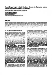
performance meta-tool, referred to as p-platform, is outlined in Fig. 1. Each layer of a pplatform describes a typical concern of a performance modeling study and we propose to organize the interaction between different submodules by means of layers, communicating through standardized meta-languages. In particular we suggest the use of XML as a possible implementation of a meta-language used to describe the interfaces between the layers. The ability of integrate different performance tools into a public framework would substantially improve the robustness and scale of current performance tools. It would also give the ability to users to select the components that best fit the goals of the performance study. The number of components required in the analysis is not fixed and depends on the objectives. Furthermore, the component of a layer can be skipped, for example one may evaluate a Markov model without using any high-level modeling language. According to the p-platform description, main steps of a performance study would be: 1. analysis of the intended use of the model based on the study’s objectives; identification of the best technique to be used to describe the problem and its characteristics; 2. identification of the solution algorithm required to produce the type of results needed, e.g., equilibrium or transient values, exact or approximate solutions; 3. design of the experiment to be undertaken through the manager module, e.g, whatif, single run, optimization technique; 4. selection of the computing infrastructure to be used to run the numerical or simulation algorithms, single server, cluster, cloud, web, etc. Although the principles outlined are simple, to the best of the authors’ knowledge integration via XML has been poorly adopted by current performance modeling tools. The only notable exceptions are the Java Modelling Suite which coordinates data exchange between modules using XML files, the ongoing performance interchange format project PMIF [24, 25], and the Petri Net Markup Language PNML 35 which is supported by a growing number of PN tools. A possible explanation for this is that the majority of the tools have been developed started from the 80s, therefore according to the software engineering principles of the time. We believe that open release of the source code through open platforms such as Sourceforge would represent a first step in the right direction of helping external groups provide ideas, report bugs, and discuss in forums the issues we have outlined in this section.

8 Conclusions In this paper, we have reviewed past and present efforts towards implementing software tools to support performance evaluation activities. Our analysis has revealed the area to be still very active, with a number of new simulation and analysis techniques still being proposed for classic models such as queuing networks and Petri nets. We have also argued that the recent advent of standardized data exchange languages such as XML opens new opportunities towards integrating existing community efforts into larger performance evaluation frameworks. To support this idea, we have outlined a performance meta-tool architecture, named p-platform, that provides high-level intuition on the basic blocks needed to define such frameworks. 35

http://www.pnml.org/

GUI & Model Definition Languages

Drag&Drop of Components

Model definition with Wizards

Languages for model description

XML Interface

Experiment Manager

Equilibrium solution

What-if Analysis

Transient Analysis

Model Validation

Optimization Objectives

XML Interface

High-level Modeling Languages

Queueing Networks

Petri Nets

Fault Trees

Stochastic Process Algebra

Fluid & Hybrid Models

XML Interface

Solution Techniques

Markov chains

Simulation

Approximate Bounds

Exact Product Form

XML Interface

Computational Infrastructure

Single Server

Cloud

Grid

Web

Fig. 1. Main components of the architecture of a performance meta-tool, referred to as p-platform.

References 1. General purpose systems simulator iii user’s manual. Technical Report Form H20-0163, IBM, 1965. 2. P. Buchholz, G. Ciardo, S. Donatelli, and P. Kemper. Complexity of memory-efficient kronecker operations with applications to the solution of markov models. INFORMS Journal on Computing, 12(3):203–222, 2000. 3. J. P. Buzen. Computational algorithms for closed queueing networks with exponential servers. Comm. of the ACM, 16(9):527–531, 1973. 4. J. P. Buzen and al. Best/1 - design of a tool for computer system capacity planning. In Proc. of the 1978 National Computer Conf., pages 447–455. AFIPS Press, 1978. 5. G. Carlson. A user’s view of hardware performance monitors. In Proc. IFIP Congress 71, pages 128–132. North-Holland, 1971.

6. G. Casale, R.R.Muntz, and G. Serazzi. Tools for computer performance modeling and reliability analysis. ACM Performance Evaluation Review, 36(4), 2009. 7. G. Chiola, C. Dutheillet, G. Franceschinis, and S. Haddad. Stochastic well-formed colored nets and symmetric modeling applications. Computers, IEEE Transactions on, 42(11):1343 –1360, nov 1993. 8. G. S. Fishman. Statistical analysis for queueing simulations. Management Science, 20, 3:363–369, 1973. 9. M. Gribaudo. Fspnedit: a fluid stochastic petri net modeling and analysis tool. In Proc. of Tools of Aachen 2001, pages 24–28, 2001. 10. P. Heidelberger and P. D. Welch. A spectral method for confidence interval generation and run length control in simulations. Comm. of the ACM, 24(4):233–245, 1981. 11. D. J. Herman. Scert: a computer evaluation tool. Datamation, 13(2):26–28, 1967. 12. D. J. Herman and F. Ihrer. The use of a computer to evaluate computers. In Proc. Conf. 1964 SJCC, Washington DC, pages 383–395. Spartan Books, 1964. 13. J. Hillston. Fluid flow approximation of pepa models. In QEST, 2005., pages 33 – 42, 19-22 2005. 14. K. Jensen. Coloured Petri Nets: Basic Concepts, Analysis Methods, and Practical Use (2nd edition). Springer, 1997. 15. D. Kartson, G. Balbo, S. Donatelli, G. Franceschinis, and G. Conte. Modelling with Generalized Stochastic Petri Nets. John Wiley & Sons, Inc., New York, NY, USA, 1994. 16. S. S. Lavenberg. A perspective on queueing models of computer performance. Performance Evaluation, 10(1):53–76, 1989. 17. H. M. Markowitz, B. Hausner, and H.W.Karr. Simscript: a simulation programming language. Prentice Hall, 1963. 18. A. Martens, H. Koziolek, S. Becker, and R. Reussner. Automatically improve software architecture models for performance, reliability, and cost using evolutionary algorithms. In WOSP/SIPEW, pages 105–116, 2010. 19. S. Montani, L. Portinale, A. Bobbio, and D. Codetta-Raiteri. Radyban: A tool for reliability analysis of dynamic fault trees through conversion into dynamic bayesian networks. Reliability Engineering and System Safety, 93(7):922 – 932, 2008. Bayesian Networks in Dependability. 20. N. R. Nielsen. Computer simulation of computer system performance. In Proc. of ACM National Meeting, pages 581–590, 1967. 21. K. Pawlikowski. Steady-sate simulation of queueing processes: A survey of problems and solutions. ACM Computing Surveys, 22(2):123–168, 1990. 22. C. H. Sauer and K. M. Chandy. Computer Systems Performance Modeling. Prentice-Hall, 1981. 23. D. Saure, P. Glynn, and A. Zeevi. A linear programming algorithm for computing the stationary distribution of semi-martingale reflecting brownian motion. under submission,. 24. C. Smith and C. Llado. Performance model interchange format (pmif 2.0): Xml definition and implementation. In In Proc. of QUEST’04. IEEE Press, 2004. 25. C. Smith, C. Llad´o, and R. Puigjaner. Performance model interchange format (pmif 2): A comprehensive approach to queueing network model interoperability. Perform. Eval., 67(7):548–568, 2010. 26. W. J. Stewart. Introduction to the Numerical Solution of Markov Chains. Princeton University Press, Princeton, NJ, USA, 1994. 27. K. S. Trivedi, A. Bobbio, G. Ciardo, R. German, A. Puliafito, and M. Telek. Non-markovian petri nets. In SIGMETRICS ’95/PERFORMANCE ’95, pages 263–264, New York, NY, USA, 1995. ACM.