Tools for Structured Matrix Computations: Stratifications ... - DiVA Portal

Tools for Structured Matrix Computations: Stratifications and Coupled Sylvester Equations

Andrii Dmytryshyn

PhD Thesis

D EPARTMENT OF C OMPUTING S CIENCE U ME A˚ U NIVERSITY

Department of Computing Science Ume˚a University SE-901 87 Ume˚a, Sweden [email protected] c 2015 by Andrii Dmytryshyn Copyright

c Society for Industrial and Applied Mathematics, 2015 Except Paper I, c Elsevier, 2013 Paper II, c A. Dmytryshyn, S. Johansson, and B. K˚agstr¨om, 2013 Paper III, c Society for Industrial and Applied Mathematics, 2014 Paper IV, c A. Dmytryshyn, S. Johansson, B. K˚agstr¨om, and P. Van Dooren, 2015 Paper V, c A. Dmytryshyn, 2015 Paper VI, c A. Dmytryshyn, S. Johansson, and B. K˚agstr¨om, 2015 Paper VII,

ISBN 978-91-7601-379-3 ISSN 0348-0542 UMINF 15.18 Printed by Print & Media, Ume˚a University, 2015

Abstract

Developing theory, algorithms, and software tools for analyzing matrix pencils whose matrices have various structures are contemporary research problems. Such matrices are often coming from discretizations of systems of differential-algebraic equations. Therefore preserving the structures in the simulations as well as during the analyses of the mathematical models typically means respecting their physical meanings and may be crucial for the applications. This leads to a fast development of structure-preserving methods in numerical linear algebra along with a growing demand for new theories and tools for the analysis of structured matrix pencils, and in particular, an exploration of their behaviour under perturbations. In many cases, the dynamics and characteristics of the underlying physical system are defined by the canonical structure information, i.e. eigenvalues, their multiplicities and Jordan blocks, as well as left and right minimal indices of the associated matrix pencil. Computing canonical structure information is, nevertheless, an ill-posed problem in the sense that small perturbations in the matrices may drastically change the computed information. One approach to investigate such problems is to use the stratification theory for structured matrix pencils. The development of the theory includes constructing stratification (closure hierarchy) graphs of orbits (and bundles) that provide qualitative information for a deeper understanding of how the characteristics of underlying physical systems can change under small perturbations. In turn, for a given system the stratification graphs provide the possibility to identify more degenerate and more generic nearby systems that may lead to a better system design. We develop the stratification theory for Fiedler linearizations of general matrix polynomials, skew-symmetric matrix pencils and matrix polynomial linearizations, and system pencils associated with generalized state-space systems. The novel contributions also include theory and software for computing codimensions, various versal deformations, properties of matrix pencils and matrix polynomials, and general solutions of matrix equations. In particular, the need of solving matrix equations motivated the investigation of the existence of a solution, advancing into a general result on consistency of systems of coupled Sylvester-type matrix equations and blockdiagonalizations of the associated matrices.

iii

iv

¨ Popularvetenskaplig sammanfattning

Verktyg f¨or strukturerade matrisber¨akningar: Stratifieringar och kopplade Sylvester-ekvationer Ett differential-algebraiskt ekvationssystem (DAE) representerar ofta en matematisk modell av ett verkligt fysikaliskt system. En modell kan till exempel beskriva ett mekaniskt system, ett elektriskt n¨atverk, eller en reaktion i en kemisk process. Att designa och analysera en DAE-modell a¨ r ofta ett komplext problem som kr¨aver h¨ogkvalitativa matematiska teorier och ber¨akningsverktyg. Parametrarna och datat a¨ r ofta p˚averkade av olika typer av st¨orningar och dessutom kan det finnas fel i sj¨alva modellbeskrivningen. Systemegenskaperna hos den DAE-modell vi betraktar ges av olika kanoniska former som ber¨aknas utifr˚an en representation i termer av matriser eller matrisknippen (par av matriser). Popul¨art sagt kan en matris ses som en stor tabell (flera rader och kolumner) med tal. Ett (linj¨art) matrisknippe best˚ar i sin tur av tv˚a matriser och relaterar till det s.k. generaliserade egenv¨ardesproblemet. I detta sammanhang beskriver egenv¨ardena dynamiken hos en DAE-modell och ger information om vilka systemvariabler som svarar mot snabba respektive mer l˚angsamma f¨orlopp. Datamatriserna (matriser och matrisknippen) har ofta n˚agon typ av struktur. Exempel p˚a strukturer a¨ r olika symmetriegenskaper hos matriserna som dessutom kan ha en s.k. blockindelning. Strukturegenskaperna a¨ r direkt kopplade till fysikaliska egenskaper och f¨or att kunna g¨ora en korrekt analys av matrisrepresentationen av ett dynamiskt system a¨ r det viktigt att a¨ ven denna struktur beaktas. Detta leder till en snabb utveckling av strukturbevarande metoder i numerisk linj¨ar algebra samt till ett v¨axande behov av nya teorier och verktyg f¨or att kunna analysera hur de strukturerade matrisknippena f¨or¨andras av sm˚a st¨orningar i indata (dvs. st¨orningar i matriserna som ing˚ar i DAE-modellen) . Att ber¨akna systemegenskaper a¨ r normalt ett s.k. illa st¨allt problem, vilket betyder att sm˚a st¨orningar i indata kan ge stor p˚averkan p˚a de ber¨aknade systemegenskaperna. Ett s¨att att unders¨oka s˚adana problem a¨ r med hj¨alp av stratifieringsteori f¨or strukturerade matrisknippen. I denna avhandling g¨ors detta genom att konstruera grafer f¨or stratifieringar som i sin tur ger information f¨or en djupare f¨orst˚aelse av hur egenskaperna hos det underliggande fysikaliska systemet kan f¨or¨andras under sm˚a st¨orningar. Av s¨arskilt intresse a¨ r att kunna identifiera n¨arliggande mer degenererade

v

och mer generiska system till ett givet system. Denna kunskap kan, till exempel, leda till o¨ kad f¨orst˚aelse av hur olika typer av styr- och reglersystem kan g¨oras mer robusta. I avhandlingen utvecklar vi stratifierinsgteorier f¨or Fiedler-linj¨ariseringar av generella polynommatriser, skevsymmetriska matrisknippen och polynommatriser samt systemknippen associerade med linj¨ara tillst˚andsmodeller av dynamiska system. Alla dessa exempel svarar mot olika matrisproblem med olika blockstruktur som tas till vara och konserveras i de nya resultaten. Bidragen i avhandlingen innefattar utveckling av teori och verktyg f¨or att ber¨akna (co-)dimensioner, att p˚avisa explicita uttryck av versala deformationer, att bevisa egenskaper hos matrisknippen och polynommatriser, att kunna l¨osa matrisekvationer. I synnerhet motiverade behovet av att l¨osa matrisekvationer oss till att unders¨oka n¨ar en l¨osning existerar (eller inte) f¨or system av kopplade matrisekvationer av Sylvester-typ. Det har resulterat i ett generellt konsistensbevis f¨or system av kopplade matrisekvationer och en block-diagonalisering av de associerade matriserna. Noterbart a¨ r att detta resultat blivit tilldelat det internationellt prestigefulla SIAM Student Paper Prize 2015. Syftet med priset, enligt stadgarna, a¨ r att lyfta fram enast˚aende insatser av studenter i till¨ampad matematik, ber¨akningsteknik eller datavetenskap.

vi

Preface

This PhD Thesis consists of the following papers:

Paper I

A. Dmytryshyn and B. K˚agstr¨om. Coupled Sylvester-type matrix equations and block diagonalization1 . SIAM J. Matrix Anal. Appl., 36(2) (2015) 580–593. Awarded the SIAM Student Paper Prize 2015.

Paper II

A. Dmytryshyn, B. K˚agstr¨om, and V. V. Sergeichuk. Skew-symmetric matrix pencils: Codimension counts and the solution of a pair of matrix equations2 . Linear Algebra Appl., 438(8) (2013) 3375–3396.

Paper III

A. Dmytryshyn, S. Johansson, and B. K˚agstr¨om. Codimension computations of congruence orbits of matrices, skew-symmetric and symmetric matrix pencils using Matlab. Report UMINF 13.18, Dept. of Computing Science, Ume˚a University, Sweden, 2013.

Paper IV

A. Dmytryshyn and B. K˚agstr¨om. Orbit closure hierarchies of skewsymmetric matrix pencils1 . SIAM J. Matrix Anal. Appl., 35(4) (2014) 1429–1443.

Paper V

A. Dmytryshyn, S. Johansson, B. K˚agstr¨om, and P. Van Dooren. Geometry of spaces for matrix polynomial Fiedler linearizations. Report UMINF 15.17, Dept. of Computing Science, Ume˚a University, Sweden, 2015.

Paper VI

A. Dmytryshyn. Structure preserving stratification of skew-symmetric matrix polynomials. Report UMINF 15.16, Dept. of Computing Science, Ume˚a University, Sweden, 2015.

Paper VII A. Dmytryshyn, S. Johansson, and B. K˚agstr¨om. Canonical structure transitions of system pencils. Report UMINF 15.15, Dept. of Computing Science, Ume˚a University, Sweden, 2015.

1 2

Reprinted by permission of Society for Industrial and Applied Mathematics. Reprinted by permission of Elsevier.

vii

In addition to the papers included in the thesis, the following four publications were written within the studies: A.R. Dmytryshyn, V. Futorny, and V.V. Sergeichuk. Miniversal deformations of matrices of bilinear forms. Linear Algebra Appl., 436(7) (2012) 2670–2700. A. Dmytryshyn, B. K˚agstr¨om, and V.V. Sergeichuk. Symmetric matrix pencils: Codimension counts and the solution of a pair of matrix equations. Electron. J. Linear Algebra, 27 (2014) 1–18. A. Dmytryshyn, V. Futorny, and V.V. Sergeichuk. Miniversal deformations of matrices under *congruence and reducing transformations. Linear Algebra Appl., 446 (2014) 388–420. A. Dmytryshyn, V. Futorny, B. K˚agstr¨om, L. Klimenko, and V.V. Sergeichuk. Change of the congruence canonical form of 2-by-2 and 3-by-3 matrices under perturbations and bundles of matrices under congruence. Linear Algebra Appl., 469 (2015) 305–334.

viii

Acknowledgements

First of all I would like to thank my supervisor Prof. Bo K˚agstr¨om for making this Thesis possible as well as the working process joyful. Despite his dedication to numerous activities, Bo is always happy to share his knowledge and experience through fruitful, interesting, and full of wisdom discussions that I enjoy a lot. I very much appreciate the time he spends (often in evenings) working with me as well as the patience he demonstrates answering my questions and commenting my writing. Not the least, I also want to thank for our every-day communication, which has been frank and encouraging, revealing Bo as a sincere person and a strong leader. It has been a pleasure and honour to work with you Bo! I am very grateful to my co-supervisor Dr. Stefan Johansson for a number of discussions on both theory and practical aspects of our research problems. Stefan is always kind and patient to give many valuable comments on various drafts. I also appreciate his invaluable support when doing the implementations of the theoretical results. In particular, Stefan introduced me to StratiGraph and the MCS Toolbox. Both of these key software tools were originally developed by Pedher Johansson – thank you! Many thanks to Prof. Vladimir V. Sergeichuk for presenting the world of miniversal deformations to me, which resulted in a productive collaboration. His constructive suggestions and insightful remarks are always helpful. Thanks to Prof. Paul Van Dooren for our recent fruitful discussions and collaboration. I am also grateful to all the staff at the Departments of Computing Science, UMIT Research Lab, and HPC2N, in particular, to the members of our research group for the friendly working environment and great atmosphere. I owe my deepest gratitude to my family, especially to my parents and to Filippa for the permanent support and love. Thank you family Sandberg for sharing with me many warm and joyful moments, as well as for familiarizing me with the Swedish traditions. My thanks also go to my friends all around the world for the shared time and fun both virtually and when we meet. Financial support has been provided by the Swedish Research Council (VR) under grants A0581501 and E0485301, and eSSENCE (essenceofescience.se), a strategic collaborative e-Science programme funded by the Swedish Government via VR. Thank you all! Andrii Ume˚a, November 2015

ix

x

Contents

1

Introduction 1.1 Sylvester-type matrix equations 1.2 Block diagonalization of matrices 1.3 Coupled Sylvester-type matrix equations and block diagonalization 1.4 Canonical matrices 1.5 The solution of matrix equations 1.6 Orbits and bundles 1.7 Codimension computations and Matrix Canonical Structure Toolbox 1.8 Versal deformations 1.9 Orbit and bundle stratifications 1.10 Orbit closure hierarchies of skew-symmetric matrix pencils 1.11 Stratification of matrix polynomials 1.12 Stratification of skew-symmetric matrix polynomials 1.13 Stratification of pencils associated with nonsingular generalized statespace systems 1.14 Summary of the main contributions

1 2 3 4 8 10 11 13 14 15 16 18 20 22 23

Paper I

33

Paper II

49

Paper III

73

Paper IV

117

Paper V

135

Paper VI

165

Paper VII

193

xi

xii

Chapter 1

Introduction Description of mechanical systems, electrical networks, and chemical reactions typically leads to differential-algebraic equations (DAE). To analyse a DAEmodel may be a hard problem, requiring complex mathematical theories and tools. In particular, to reveal the dynamics of the underlying system, we often need to compute the canonical information, e.g., eigenvalues and eigenstructures, of the matrices coming from a discretization of the DAE. In general, these problems are ill-posed in the sense that small perturbations in the matrices may drastically change the computed canonical information. The problems become even more challenging if the involved matrices have additional structures, e.g., symmetries and/or blocking. Preserving these structures in the simulations as well as during the analyses of the mathematical models often means respecting their physical meanings and may be crucial for the applications. Therefore the development of structure-preserving methods is a rapidly growing area of research in numerical linear algebra with significant progress during the recent years. Canonical information associated with a number of DAEs can be obtained by the investigation of just a pair of matrices with a certain structure, so called structured matrix pencils1 , which in turn, demands new theory, algorithms, and software tools for their analysis, and in particular, an exploration of their behaviour under perturbations. One approach to investigate how small perturbations affect the canonical information of (structured) matrix pencils and thus characteristics of the underlying physical system, is developing the stratification theory (constructing closure hierarchies) of these matrix pencils. In turn, the stratification theory provides the possibility to identify more degenerate and more generic nearby systems to a given system. This Thesis addresses problems of how eigenvalues, associated Jordan blocks, as well as left and right minimal indices of structured matrix pencils change under structure-preserving perturbations. The considered structures include symmetries and blocking coming from generalized state-space systems and lin1 Formally: For two m × n matrices A and B a matrix pencil is defined as A − λB, where λ is a scalar parameter.

1

earzations of matrix polynomials. Nevertheless, the described problems require both using and contributing to a number of mathematical disciplines, including matrix computations, classificational problems in linear algebra, matrix polynomials, versal deformations, geometry of matrix spaces, matrix equations, etc. Note that Papers I–VII are the papers [38], [39], [34], [37], [36], [30], and [35], respectively, in the bibliography of Chapter 1.

1.1

Sylvester-type matrix equations

Matrix equations appear frequently in various engineering applications. One important type is Sylvester matrix equations [85] of the following form: AX + XB = C,

where X is an unknown matrix, and A, B, C are given matrices of conforming sizes. Similarly, these equations may have two unknown matrices, X and Y : AX + Y B = C.

More recently, a lot of attention is devoted to so called ⋆-Sylvester2 matrix equations, where the unknown matrices may also appear (conjugate) transposed: AX + X ⋆ B = C.

Considering a few of the equations above that share some of the unknown matrices lead to the various systems of Sylvester-type matrix equations. In the most general case, we have systems of coupled matrix equations including an arbitrary mix of Sylvester and ⋆-Sylvester equations, i.e., systems of n1 + n2 matrix equations with m unknown matrices Ai Xk ± Xj Bi = Ci ,

Fi′ Xk′ ± Xj⋆′ Gi′

= Hi ′ ,

i = 1, . . . , n1 ,

i′ = 1, . . . , n2 ,

(1.1)

where k, j, k ′ , j ′ ∈ {1, . . . , m}, each unknown Xl is rl × cl , l = 1, . . . , m, all other matrices are of conforming sizes, and Ai , Bi , Ci , Fi′ , Gi′ , Hi′ , and Xk are matrices over the field F of characteristic different from two. This includes matrices over real or complex numbers which appear frequently in various applications. The indices k and j depend on i (are integer functions of i) as well as k ′ and j ′ depend on i′ which reflect that different equations may share the same or have different unknown matrices. The same unknown matrices may appear in the matrix equations of the same type, as well as in the matrix equations of different types. This couples all equations on the intra- and inter-type levels, respectively. Depending on the choice of n1 , n2 , and m as well as the positioning (or indexing) 2 We use the (⋅)⋆ -operator in X ⋆ to denote the matrix transpose X T or the matrix conjugate transpose X H , for any matrix X. Thus ⋆-Sylvester means T-Sylvester or H-Sylvester. Note that * is often used instead of H as we do in this Thesis.

2

of the unknown matrices, there exist many special cases of (1.1) which have already been studied in the literature, see more in Paper I, Sections 1–2. Popularity of Sylvester and ⋆-Sylvester matrix equations is due to their broad importance in many applications; for example robust, optimal, and singular system control, signal processing, filtering techniques, feedback, model reduction, numerical solution of differential equations, e.g., see [7, 9, 16, 18, 38, 90, 91] and references therein. Let us also point out that Sylvester matrix equations arise in computing stable eigendecompositions of matrices and matrix pencils [24], and ⋆-Sylvester matrix equations are closely related with palindromic matrix pencils, e.g., analysis of associated deflating subspaces [10]. Robust and efficient algorithms, software for solving (⋆-)Sylvester-type equations have been developed, e.g., see [18, 41, 65], RECSY [61, 62], SCASY [51, 52], and a recent survey [82]. Before solving such equations it is natural to ask about the existence of the solution (i.e. consistency) as well as its uniqueness.

1.2

Block diagonalization of matrices

In all types of matrix computations, the simplest objects are diagonal matrices, i.e. all entries are zeros except the diagonal elements. This stimulates development of various reduction techniques that allow to diagonalize matrices and thus simplify problems that they represent. However, very few matrix problems actually allow complete diagonalization. A compromise is to reduce the problem to block-diagonal form A 0 [ ], 0 B in which A and B are square matrices, possibly of different sizes, and zeros denote conforming zero matrices. For many problems we are interested in block diagonalizing several matrices simultaneously, e.g., reducing n matrices to the forms A 0 A 0 A 0 [ 1 ], [ 2 ], ... , [ n ] 0 B1 0 B2 0 Bn

in which the square matrices A1 , A2 , . . . , An , all are of the same size as well as B1 , B2 , . . . , Bn (but Ai and Bi can be of different sizes). Block diagonalization allows to decouple the problem into two or more independent problems of smaller sizes. The transformations used for reductions depend on the problems and typically can be expressed as matrix multiplications on the left and right-hand sides with certain (nonsingular) matrices; a number of examples of possible transformations, appearing in applications, are presented in Section 1.3 and Paper I. An important case is the block diagonalzation of a matrix (or several matrices) that are already in block triangular form(s), e.g., reducing a single matrix A [ 0

C ] B

to

3

A [ 0

0 ]; B

or reducing a pair of matrices A ([ 1 0

C1 A ],[ 2 B1 0

C2 ]) B2

([

to

A1 0

0 A ],[ 2 B1 0

0 ]) . B2

Studying separations between two matrices or matrix pairs is an example of where such problems appear [24]. If the nonzero blocks are instead on the antidiagonals, we call it block antidiagonalization, leading to matrices of the form 0 [ F1

1.3

G1 0 ], [ 0 F2

G2 0 ], ... , [ 0 Fn

Gn ]. 0

Coupled Sylvester-type matrix equations and block diagonalization

In 1952, Roth revealed the connection between the existence of a solution (i.e., the consistency) for a Sylvester matrix equation and the similarity relation between two particular block-matrices constructed from the matrix coefficients of the considered Sylvester matrix equation [81]: Theorem 1. The matrix equation AX − XB = C has a solution X if and only A C A 0 if there exists a nonsingular matrix P such that P −1 [ ]P = [ ]. 0 B 0 B

Since then, similar results have been published for a number of other Sylvester and more recently ⋆-Sylvester matrix equations as well as for some systems of matrix equations (e.g., see Table 1.1 or [6, 18, 53, 68, 81, 84, 93, 94]3 ). These results are often referred in the literature as Roth’s theorems. In Paper I, we prove a general Roth’s type theorem for systems of matrix equations consisting of an arbitrary mix of Sylvester and ⋆-Sylvester equations. In full generality, we derive consistency conditions by proving that such a system has a solution if and only if the associated set of 2 × 2 block matrix representations of the equations are block diagonalizable by (linked) equivalence transformations. In particular, all known Roth’s theorems are partial cases of the main theorem in Paper I, see the last column of Table 1.1. The simplicity in the statement of this main theorem allows us to present it immediately. 3 In some of these papers consistency is just one of the investigated properties for a particular matrix equation [6, 18, 84]; other papers are completely devoted to the consistency of matrix equations or systems thereof [53, 68, 81, 93, 94].

4

Theorem 2. The system of n1 + n2 matrix equations with m unknown matrices Ai Xk − Xj Bi = Ci ,

Fi′ Xk′ + Xj⋆′ Gi′

= Hi′ ,

i = 1, . . . , n1 ,

i = 1, . . . , n2 , ′

(1.2)

(1.3)

where j, k, j ′ , k ′ ∈ {1, . . . , m}, has a solution (X1 , X2 , . . . , Xm ) if and only if there exist nonsingular matrices P1 , P2 , . . . , Pm such that A Pj−1 [ i 0

0 Pj⋆′ [ Fi′

Ci A ]P = [ i Bi k 0

Gi′ 0 ]P ′ = [ Hi′ k Fi′

0 ], Bi

Gi′ ], 0

i = 1, . . . , n1 ,

i′ = 1, . . . , n2 .

(1.4) (1.5)

In Theorem 2 each unknown Xl is rl × cl , l = 1, . . . , m, and the other matrices are of conforming sizes. We may have n1 = 0 or n2 = 0 which would mean that matrix equations (1.2) or (1.3) are absent as well as the conditions (1.4) or (1.5), respectively. Theorem 2 relates the consistency, i.e. the property of having a solution, of a system of matrix equations (1.2)–(1.3) to the block diagonalization and the block anti-diagonalization of the corresponding set of block-triangular matrices (1.4)–(1.5). Notably, Theorem 2 also covers the cases of existence of (skew-)hermitian or (skew-)symmetric solutions since we can add the equations Xk ± Xk⋆ = 0 for the variables we want to satisfy the corresponding condition. These cases are an additional motivation to consider systems with both Sylvester and ⋆-Sylvester equations ([94] shows this result for one equation). Generality of our result: In contrast to the known partial cases, where n1 , n2 , and m are fixed and often small integers, Theorem 2 does not put any restrictions on the numbers of equations n1 and n2 , or unknowns m. Note that not only n1 , n2 , and m define the settings for Theorem 2 but also the positions of the unknowns in every equation of the system (1.2)–(1.3). Again our result covers all the orders while the known partial cases have one fixed order each. To illustrate our result and to easily distinguish the partial cases, we use a tool from representation theory and associate a graph with each particular case of Theorem 2. This method of “visualization” is inspired by the representation theory of quivers and mixed type graphs [56], i.e. graphs with both directed and undirected edges, where a set of linear mappings is associated with directed graphs as well as a set of linear and bilinear (or sesquilinear) mappings is associated with mixed type graphs. Now, through Theorem 2 we essentially associate a graph to a system of Sylvester and ⋆-Sylvester matrix equations. Until now Roth’s type theorems were proven for systems (and the matrix equivalence relations) associated with one graph, for example [45, 81, 93] (see also Figure 1.1) or one type of graphs, for example [53, 68] (see also the graphs in Figure 1.2 for any n). We show that Roth’s theorems hold for the systems (and the matrix equivalence relations) associated with any graph, e.g., the graphs in Figures 1.1–1.3.

5

[

[

V

A 0

A1 0

C1 ] B1

V

C ] B

W [

A2 0

C2 ] B2

Figure 1.1: Graphs associated with two Roth’s theorems. Both graphs are particular cases of Theorem 2 and included in Table 1.1: The left graph corresponds to AX − XB = C and the similarity of the block matrices [45, 81]; The right graph corresponds to A1 X1 − X2 B1 = C1 and A2 X1 − X2 B2 = C2 and the strict equivalence of the block matrices [6, 84, 93]. [

[

An−1 0

An 0

Cn−1 ] Bn−1

Cn ] Bn

...

[

V

...

C1 ] B1

A1 0

[

C2 ] B2

A2 0

Figure 1.2: The graph corresponds to systems of n Sylvester equations with one unknown matrix and simultaneous similarity of the block matrices (Roth’s theorems from [53, 68]); see also Table 1.1.

[

V1

[

A1 0

C1 ] B1

An 0

Cn ] Bn

V2 . . .

. . . Vn−1

[

An−1 0

Cn−1 ] Bn−1

Vn

Figure 1.3:

The graph corresponds to systems of n Sylvester equations with n unknown matrices in a cyclic order, associated with the periodic eigenvalue problem; see also the last row of Table 1.1.

Although the associated graphs are not used for the proofs they are convenient for the problem description and identification, see more in Section 3 of Paper I. Theorem 2 can also be used for systems of matrix equations that are reducible to systems of Sylvester and ⋆-Sylvester equations (e.g., by introducing new variables). Systems of Stein-type matrix equations Ai Xk Ki ± Li Xj Bi = Ci ,

Fi′ Xk′ Mi′ ± Ni′ Xj⋆′ Gi′ = Hi′ ,

i = 1, . . . , n1 ,

i′ = 1, . . . , n2 ,

where j, k, j ′ , k ′ ∈ {1, . . . , m}, are one important class of such systems and in Section 6 of Paper I we derive a consistency theorem for them. 6

System of matrix equations AX − XB = C

A1 X − XB1 = C1 , ...

An X − XBn = Cn , AX1 − X2 B = C

A1 X1 − X2 B1 = C1 ,

A2 X1 − X2 B2 = C2 , A1 X1 − X2 B1 = C1 , ...

An X1 − X2 Bn = Cn , A1 X1 − X2 B1 = C1 ,

A2 X3 − X2 B2 = C2 , F X + X⋆G = H ⋆

F 1 X + X G 1 = H1 , ⋆

...

Fn X + X Gn = Hn , AX − XB = C, ⋆

X − X = 0,

A1 X1 − X2 B1 = C1 ,

A2 X2 − X1 B2 = C2 ,

A1 X1 − X2 B1 = C1 , A2 X2 − X3 B2 = C2 , ...

An−1 Xn−1 − Xn Bn−1 = Cn−1 , An Xn − X1 Bn = Cn ,

Reference

Relation on the corresponding matrices

1952, [81]

⇐⇒

P −1 [

1977, [45]

⇐⇒

1985, [53]

⇐⇒

P

2012, [68]

⇐⇒ 1952, [81] ⇐⇒ 1977, [45]

⇐⇒

1994, [93]

⇐⇒

1994, [84]

⇐⇒

A 0

−1 Ai [ 0

A Ci ]P = [ i 0 Bi

−1 [A P2 0

A C ] P1 = [ 0 B

⇐⇒ 1985, [53] ⇐⇒ 1994, [93]

⇐⇒

2012, [68]

⇐⇒

2012, [68]

⇐⇒ ⇐⇒ ⇐⇒

Ci A ] P1 = [ i Bi 0

0 ] Bi

−1 A P2 [ 1 0

A C1 ] P1 = [ 1 B1 0

0 ] B1

P

⋆

[

0 F

0 Fi

−1 A P [ 0

1994, [94]

⇐⇒

⋆ 0 P [ I

−1 A P2 [ 1 0

⇐⇒

−1 A P1 [ 2 0 −1 A Pi+1 [ i 0

⇐⇒

A C2 ] P1 = [ 2 B2 0

0 ] B2

i = 1, . . . , n

A C2 ] P3 = [ 2 B2 0 G 0 ]P = [ H F Gi 0 ]P = [ Hi Fi

0 ] B2 G ] 0 Gi ] 0

i = 1, . . . , n

C A ]P = [ B 0

−I 0 ]P = [ 0 I

C1 A ] P1 = [ 1 B1 0 A C2 ] P2 = [ 2 B2 0 Ci A ] Pi = [ i Bi 0

i = 1, . . . , n,

Table 1.1:

0 ] B

−1 A P2 [ i 0

P⋆ [

2014, [15]

i = 1, . . . , n

0 ] B1

2011, [18]

⇐⇒

0 ] Bi

A C1 ] P1 = [ 1 0 B1

−1 A P2 [ 2 0

1994, [94]

0 ] B

−1 A P2 [ 1 0 −1 A P2 [ 2 0

1996, [6]

A C ]P = [ 0 B

0 ] B

−I ] 0

0 ] B1 0 ] B2

0 ] Bi

Pn+1 ∶= P1

The case of Theorem 2 n1 = 1, n2 = 0 m=1

n1 = n, n2 = 0

m=1

n1 = 1, n2 = 0 m=2

n1 = 2, n2 = 0 m=2

n1 = n, n2 = 0

m=2

n1 = 2, n2 = 0 m=3

n1 = 0, n2 = 1 m=1

n1 = 0, n2 = n

m=1

n1 = 1, n2 = 1 m=1

n1 = 2, n2 = 0 m=2

“cyclic order”

n1 = n, n2 = 0 m=n

“cyclic order”

Some known and (as an example two) new Roth’s theorems are presented: each row corresponds to a theorem and is a particular case of Theorem 2. The last two rows contain Roth’s theorems for contragredient matrix pencils and the general periodic eigenvalue problem, which surprisingly, do not seem to be explicitly stated and published before. The table is structured as follows: The first column shows systems of matrix equations considered; each system has a solution if and only if the corresponding relation to the block-matrices (in the third column) holds for some nonsingular matrices Pi ; in the second column we cite the papers and years of publication for the results. In the last column, we state the values of n1 , n2 , and m to obtain these results from Theorem 2.

7

The consistency conditions for systems of matrix equations have been stated not only through the corresponding equivalence relations of the block matrices but also via, e.g., ranks or generalized inverses [5, 90, 91]. Nevertheless, many of these conditions can be derived from the corresponding equivalence relations of the block triangular matrices in Theorem 2. Roth’s theorems became classical results that are used in pure and applied mathematics as well as in scientific computing. Paper I opens possibilities for other new results at a general level.

1.4

Canonical matrices

We recall the Jordan canonical form of matrices, the Kronecker canonical form of general matrix pencils, and canonical form of skew-symmetric matrix pencils under congruence. Hereafter, all matrices that we consider are over the field of complex numbers. For each k = 1, 2, . . ., define the k × k matrices ⎡µ 1 ⎢ ⎢ µ ⋱ ⎢ Jk (µ) ∶= ⎢ ⎢ ⋱ ⎢ ⎢ ⎣

⎡1 ⎢ ⎢ ⎢ Ik ∶= ⎢ ⎢ ⎢ ⎢ ⎣

⎤ ⎥ ⎥ ⎥ ⎥, 1 ⎥⎥ µ⎥⎦

1

⎤ ⎥ ⎥ ⎥ ⎥, ⋱ ⎥⎥ 1⎥⎦

where µ ∈ C, and for each k = 0, 1, . . ., define the k × (k + 1) matrices ⎡0 ⎢ ⎢ Fk ∶= ⎢ ⎢ ⎢ ⎣

1 ⋱

⋱ 0

⎤ ⎥ ⎥ ⎥, ⎥ 1⎥⎦

⎡1 ⎢ ⎢ Gk ∶= ⎢ ⎢ ⎢ ⎣

0 ⋱

⋱ 1

⎤ ⎥ ⎥ ⎥. ⎥ 0⎥⎦

All non-specified entries of Jk (µ), Ik , Fk , and Gk are zeros. An n×n matrix A is called similar to C if and only if there exists a nonsingular matrix W such that W −1 AW = C (notably the same type of transformation is applied to the block-matrices in Theorem 1, Section 1.3).

Theorem 3. 4 ([47, Sect. VII, 7], [55, Ch. 3]) Each n × n matrix A is similar to a direct sum of Jk (µ), µ ∈ C, which is uniquely determined up to permutation of summands.

The blocks Jk (µ) are called Jordan blocks and the canonical form from Theorem 3 is the Jordan canonical form (JCF) of a matrix A. Recall that the complex number µ is an eigenvalue and A may have up to n different eigenvalues µi . Each simple eigenvalue µi has only one Jordan block J1 (µi ) in the JCF. Each multiple eigenvalue µi , i.e. µi with algebraic multiplicity ≥ 2, has one or several associated Jordan blocks Jk (µi ). The number of Jk (µi ) blocks is called the geometric multiplicity of µi . We often use the term canonical structure information to describe the structural information provided by the JCF, 4 Jordan canonical form recalled here is used in this introductory part to illustrate some concepts that are utilized for the more complex canonical forms in Papers II–VII.

8

i.e. eigenvalues and their multiplicities as well as the numbers and the sizes of the associated Jordan blocks. Similarly, an m×n matrix pencil A−λB is called strictly equivalent to C −λD if and only if there exist nonsingular matrices Q and R such that Q−1 AR = C and Q−1 BR = D. Theorem 4. [47, Sect. XII, 4] Each m × n matrix pencil A − λB is strictly equivalent to a direct sum, uniquely determined up to permutation of summands, of pencils of the form Ek (µ) ∶= Jk (µ) − λIk , in which µ ∈ C, Lk ∶= Fk − λGk ,

and

LTk

∶=

FkT

Ek (∞) ∶= Ik − λJk (0),

− λGTk .

The canonical form in Theorem 4 is known as the Kronecker canonical form (KCF). The blocks Ek (µ) and Ek (∞) correspond to the finite and infinite eigenvalues, respectively, and altogether form the regular part of A − λB. The blocks Lk and LTk correspond to the right (column) and left (row) minimal indices, respectively, and form the singular part of the matrix pencil. An n × n matrix pencils A − λB with A = −AT and B = −B T is called skewsymmetric. A skew-symmetric matrix pencil A − λB is congruent to C − λD if and only if there exists a nonsingular matrix S such that S T AS = C and S T BS = D. Recall that congruence preserves skew symmetry. Theorem 5. [87] Each skew-symmetric n×n matrix pencil A−λB is congruent to a direct sum, determined uniquely up to permutation of summands, of pencils of the form 0 Hh (µ) ∶= [ −Jh (µ)T 0 Kk ∶= [ −Ik

0 Mm ∶= [ T −Fm

Jh (µ) 0 ] − λ[ −Ih 0

0 Ik ] − λ[ 0 −Jk (0)T Fm 0 ] − λ[ T 0 −Gm

Ih ], 0

Jk (0) ], 0

Gm ]. 0

µ ∈ C,

Notably, the canonical form in Theorem 5 is a “skew-symmetric analogue” of the Kronecker canonical form. The canonical structure information for (skewsymmetric) matrix pencils consists of the (distinct) eigenvalues with the sizes and the numbers of associated Jordan blocks, as well as the right and left minimal indices. Many other canonical forms are known, including those for matrices under (*)congruence [57], (skew-)symmetric/(skew-)symmetric matrix pencils [80, 87], nonsingular state-space system pencils [88]. Simplicity and beauty of the canonical forms described above are not coming for free, in particular, reductions to these forms as well as computations of the canonical structure information are sensitive to small perturbations in the matrix entries (ill-posed problems), see more in Sections 1.8–1.13 and Papers IV–VII. In practice, staircase algorithms and unitary transformations, e.g.,

9

the GUPTRI algorithm [25, 26], are used to compute the exact canonical structure information of a nearby matrix pencil. If the distance to the nearby pencil is small relative to the machine precision, this is the best we can expect in finite precision arithmetic. However, due to the ill-posedness of the problem, the computed canonical structure information may be different from the canonical structure information of the given (input) pencil.

1.5

The solution of matrix equations

Solving matrix equations with the matrix coefficients in canonical forms is a well-known problem in linear algebra. In the classical book [47, Section VIII] by F.R. Gantmacher, the homogeneous matrix equation JA Y − Y JB = 0, where JA and JB are in Jordan canonical forms, is solved. For example, this matrix equation with ⎡ ⎢ ⎢ ⎢ ⎢ JA = JB = J3 (µ) ⊕ J2 (µ) = ⎢ ⎢ ⎢ ⎢ ⎢ ⎣

has the solution

⎡ ⎢ ⎢ ⎢ ⎢ Y =⎢ ⎢ ⎢ ⎢ ⎢ ⎣

y1 0 0 0 0

y2 y1 0 y6 0

y3 y2 y1 y7 y6

y4 0 0 y8 0

y5 y4 0 y9 y8

µ 1 0 0 0 ⎤⎥ 0 µ 1 0 0 ⎥⎥ 0 0 µ 0 0 ⎥⎥ ⎥ 0 0 0 µ 1 ⎥⎥ 0 0 0 0 µ ⎥⎦

⎤ ⎥ ⎥ ⎥ ⎥ ⎥ , where yi , . . . , y9 ∈ C. ⎥ ⎥ ⎥ ⎥ ⎦

Since the coefficient-matrices JA and JB are partitioned into Jordan blocks (of sizes 3 × 3 and 2 × 2), the solution Y is constructed block-wise, i.e. each diagonal block and each off-diagonal block are treated independently. Moreover if A and B are arbitrarily square matrices and the nonsingular matrices U and V such that A = U −1 JA U and B = V −1 JB V are known, then solving a matrix equation AX − XB = 0 is equivalent to solving JA Y − Y JB = 0 with Y = U XV −1 . The solution X is then recovered by X = U −1 Y V . Notably, if A = B then our matrix equation becomes AX = XA and solving it is equivalent to describing all the matrices X that commute with A (a problem of Frobenius) [47, Section VIII]. Similarly, using the canonical forms under (*)congruence [57], the solution of the matrix equations XA + AX ⋆ = 0, where A is a square matrix, is derived in [13, 16, 17, 50]; using the KCF, the solutions of the matrix equations AX + X ⋆ B = 0, and also AX + BX ⋆ = 0, where the matrices A and B are rectangular of conforming sizes, are derived in [19] and [14], respectively. In Paper II, we establish the general solution for the homogeneous system of matrix equations X T A + AX = 0,

X T B + BX = 0, 10

(1.6)

where A = −AT and B = −B T are skew-symmetric n × n matrices. If CA − λCB is the canonical form under congruence of A − λB (see Theorem 5) and a matrix S is such that A − λB = S T CA S − λS T CB S then (1.6) is equivalent to Y T CA + CA Y = 0,

Y T CB + CB Y = 0,

with Y = S −1 XS. Since the matrix pencil CA − λCB is partitioned into blocks according to the canonical form in Theorem 5, the diagonal blocks, the offdiagonal blocks that correspond to the canonical summands of the same type, and the off-diagonal blocks that correspond to the canonical summands of different types can be treated independently and the solution can be constructed block-wise. Notably, the blocks of the solution often have Toeplitz or Hankel structures (similarly to the example on JCF above). Using the same techniques and the canonical forms of symmetric matrix pencils under congruence [87], we solve the system (1.6) with both A and B symmetric, see [40]. The matrix equation XAX = B, where A and B are both symmetric or skew-symmetric, is studied in [67]. Note the number of independent parameters in the solution of matrix equations does not depend on whether the matrix coefficients are in canonical forms or not, and is equal to the dimensions of the solution spaces. Moreover, these dimensions are closely related with the dimensions and codimensions of the corresponding matrix manifolds, as well as the homogeneous matrix equations are related to the tangent spaces of these manifolds, see Sections 1.6–1.7 and [16, 17, 39, 40]. Such relations are essentially our main motivation for studying the solutions of matrix equations with the matrix coefficients in canonical forms.

1.6

Orbits and bundles

Define an orbit of a matrix (or a matrix pencil) to be a set of matrices (or matrix pencils) with the same canonical form, e.g., an orbit of a square matrix A under similarity is a set of matrices with the same Jordan canonical form. Similarly we can define orbits for the other canonical forms mentioned in Section 1.4, but it is more general to define the orbits without using canonical matrices. In the following, we introduce some definitions in details for skew-symmetric matrix pencils. The corresponding definitions exist for the other matrix objects discussed in the Thesis. The set of skew-symmetric n × n matrix pencils congruent to A − λB forms a manifold in the complex n2 −n dimensional space (both A and B have n(n−1)/2 independent parameters). This manifold is the orbit of A − λB under the action of congruence OcA−λB = {C T (A − λB)C ∶ C ∈ GLn (C)}. (1.7) Since every skew-symmetric matrix pencil belongs to exactly one congruence

11

orbit, the whole space is an infinite union of the orbits. The vector space TA−λB ≡ {(X T A + AX) − λ(X T B + BX) ∶ X ∈ Cn×n }

(1.8)

is the tangent space to the congruence orbit of A − λB at the point A − λB. The orthogonal complement to TA−λB , with respect to the Frobenius inner product ⟨A − λB, C − λD⟩ = trace(AC ∗ + BD∗ ),

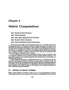
is called the normal space (denoted by NA−λB ) to the congruence orbit. Figure 1.4 illustrates the geometry of the spaces.

Figure 1.4: The tangent space TA−λB and the normal space NA−λB to the congruence orbit OcA−λB at the point A − λB.

The dimension of the orbit of A − λB is the dimension of its tangent space at the point A − λB. The codimension of the orbit A − λB, denoted cod OcA−λB , is the dimension of the normal space of its orbit at the point A − λB, which is equal to n2 − n minus the dimension of the orbit. So the dimension and the codimension of an orbit sum up to the dimension of the whole space.

All the elements of an orbit have the same fixed eigenvalues, but sometimes it is preferable to work with the sets where the values of the eigenvalues may be different while their multiplicities and canonical block structures remain the same. These sets are called bundles. Formally, two skew-symmetric matrix pencils are in the same bundle BcA−λB if and only if they have the same singular structure (the minimal indices) and the same Jordan structure except that the distinct eigenvalues may be different. Similarly, bundles are defined for matrices and matrix pencils under similarity and strict equivalence [43], respectively. Note that a bundle is an infinite union of orbits but the whole space is a finite union of bundles. For each skew-symmetric matrix pencil A − λB we define cod BcA−λB = cod OcA−λB − # {distinct eigenvalues of A − λB} . 12

(1.9)

1.7

Codimension computations and Matrix Canonical Structure Toolbox

As we mentioned in Section 1.5, there is a relation between the orbit codimensions and the dimensions of the solution spaces of the corresponding matrix equations. In some cases they are just equal to each other [16, 17], but not always. Particularly, in Paper II we show that the codimension of the congruence orbit of the skew-symmetric n × n matrix pencil A − λB is equal to the number of linearly independent solutions of (1.6) minus n. We also derive an explicit formula for the codimension of the orbit via the canonical structure information of A − λB. Note that the matrix equations (1.6) are actually coming from the representation of the tangent space (1.8). Formulas for computing the codimensions via canonical structure information are also derived for a number of other cases, including matrices under similarity (JCF) [2] [47, Section VIII], matrix pencils under strict equivalence (KCF) [23], matrices [16] and symmetric matrix pencils [40] under congruence, and matrices under *congruence [17], generalized matrix products [64], generalized state-space system pencils under feedback-injection equivalence [48] and Paper VII. To explain the reason for computing codimensions rather than dimensions, let us refer to the bundle codimensions of matrices under similarity in the singularity theory [2, 4]. For bundles of matrices under similarity (i.e., bundles for JCF) the codimension formula (1.9) remains true. Thus distinct eigenvalues that correspond to 1 × 1 Jordan blocks do not contribute to the bundle codimension. Therefore the codimensions of bundles are independent of the matrix dimensions, e.g., the bundle of J3 (µ1 ) (representing a “singularity”) has the same codimension as the bundles J3 (µ1 )⊕J1 (µ2 ), J3 (µ1 )⊕J1 (µ2 )⊕J1 (µ3 ), etc. This property remains true, for example, for regular matrix pencils under strict equivalence and regular skew-symmetric matrix pencils under congruence but fails for singular matrix pencils. Matrix Canonical Structure (MCS) Toolbox [59, 83] for Matlab5 was developed to work with matrices or matrix pencils under different transformations, e.g., similarity, congruence, equivalence, etc., and the corresponding canonical structures. Examples of functionalities include Matlab functions for creating canonical structure objects or (random) matrix example setups with a desired canonical structure information, Matlab functions that compute the codimensions of the corresponding orbits, as well as a number of auxiliary functions. It is also possible to transfer data from MCS Toolbox to StratiGraph6 and vice versa. 5 Matlab

is a registered trademark of The MathWorks, Inc. is a java-based tool developed to construct and visualize the closure hierarchy (stratification) graphs [59, 63, 83], e.g., see the graph in Figure 1.6. More details are presented in Sections 1.9–1.13. 6 StratiGraph

13

In Paper III, we extend MCS Toolbox with functionality for congruence and *congruence of matrices, as well as congruence of symmetric and skew-symmetric matrix pencils. The toolbox previously already included Matlab functions for matrices up to similarity, matrix pencils up to strict equivalence, controllability and observability pairs, as well as system pencils associated with nonsingular generalized state-space systems up to (feedback-injection) equivalence. The theoretical backgrounds and motivations for these problems are presented in [44, 59]. Whenever the canonical structure information of the matrices or the matrix pencils is known (or specified) we use it for the codimension computations, see [2, 16, 17, 23, 40, 48, 64] and Paper II. Obviously, this computation is always exact and fast for problems of any sizes. Otherwise, the codimensions are determined numerically by computing the rank and nullity of Kronecker product matrices associated with the problems. The 2n2 × n2 matrix Z (1.10) is a matrix representation of the tangent space to the congruence orbit of a skew-symmetric n × n matrix pencil A − λB at the point A − λB: AT ⊗ In + (In ⊗ A)P Z≡[ T ], B ⊗ In + (In ⊗ B)P

(1.10)

where P is the n2 × n2 permutation matrix that can “transpose” n × n matrices, i.e., vec(X T ) = P vec(X) for any n×n matrix X. The nullities of (1.10) minus n is equal to the codimensions of the congruence orbits of skew-symmetric matrix pencils. Note that the system of linear equations Z vec(X) = 0 is equivalent to (1.6). An alternative way to compute the codimensions is to calculate the number of independent parameters in the corresponding miniversal deformations [2, 28, 31, 32, 42, 49] (see also Section 1.8 for definitions).

1.8

Versal deformations

We recall that reductions to Jordan, Kronecker, or any other canonical forms mentioned in Section 1.4 are unstable operations: both the corresponding canonical forms and the reduction transformations depend discontinuously on the entries of the original matrix or matrix pencil. Therefore versal deformations [2] ̃ were introduced, i.e., a normal form to which an arbitrary family of matrices A ̃ − λB) ̃ close to a given matrix A (or matrix pencil A − λB) (or matrix pencils A ̃ can be reduced by transformations smoothly depending on the elements of A ̃ ̃ (or A − λB). Versal deformations capture all the possible changes of the investigated object and help us to understand which canonical forms matrices (or matrix pencils) may have in a neighbourhood of a given matrix (or matrix pencil). If such a form has the minimal number of independent parameters it is called miniversal deformation. This number is actually equal to the orbit’s codimension. The foundations of this theory were laid by V.I. Arnold [2, 3, 4], see also [86]. Now miniversal deformations are known for Jordan matrices [2], matrices

14

with respect to congruence [31] and *congruence [32], matrix pencils [42, 49], etc., (a more detailed list of references is given in the introduction of [31]). In particular, miniversal deformations of skew-symmetric and symmetric matrix pencils are derived in [28] and [29], respectively. For example, the miniversal deformation of J3 (µ) ⊕ J2 (µ) is ⎡ ⎢ ⎢ ⎢ ⎢ ⎢ ⎢ ⎢ ⎢ ⎢ ⎣

µ 0 ε1 ε6 ε7

1 µ ε2 0 0

0 1 µ + ε3 0 0

0 0 ε4 µ ε8

0 0 ε5 1 µ + ε9

⎤ ⎥ ⎥ ⎥ ⎥ ⎥, ⎥ ⎥ ⎥ ⎥ ⎦

where ε1 , . . . , ε9 are independent and arbitrarily small parameters (in contrast to the fully perturbed matrix that has 25 independent parameters). Versal deformations are transversal 7 to the tangent spaces; this suggests a possible way to construct them [31, 32, 49]. To be orthogonal to the tangent space, a versal deformations must lay in the corresponding normal space [42]. Algorithms constructing transformations that reduce the matrices to miniversal deformations are discussed in [76, 77]. Notably, versal deformations allow us to analyze perturbations of matrix polynomials via the study of perturbations of linearizations of such matrix polynomials, see Sections 1.11–1.12 and Papers V–VI; as well as perturbations of state-space system pencils via perturbations of the corresponding matrix pencils, see Section 1.13 and Paper VII.

1.9

Orbit and bundle stratifications

How canonical structure information changes under perturbations, e.g., the confluence and splitting of eigenvalues of a matrix, matrix pencil or polynomial, is an essential issue for understanding and predicting the behaviour of a physical system described by such matrix objects. In general, these problems are known to be ill-posed; small perturbations in the input data may lead to drastical changes in the results. The ill-posedness stems from the fact that both the canonical forms and the associated reduction transformations are discontinuous functions of the entries of involved matrices. Therefore it is important to get knowledge about the canonical forms (or canonical structure information) of the matrix objects that are close to a given one. The problem becomes even more interesting (viz. harder) if the involved matrices have structures that need to be preserved, e.g., various forms of symmetries or block structures. We investigate this problem by constructing the stratifications, i.e. the closure hierarchy graphs, of orbits and bundles of the corresponding matrix objects. Each node (vertex) of such a graph represents a system with a certain canonical structure information and there is an edge from one node to another if we can perturb the first 7 Two subspaces of a vector space are called transversal if their sum is equal to the whole space [4, Ch. 29].

15

node such that its canonical structure information becomes equal to the one of the system associated with the second node. As a result, we provide qualitative information of nearby matrix pencils and the associated canonical forms. The ways to construct the stratification graphs are already known for several matrix problems: matrices under similarity (i.e., JCF) [27, 43, 75], matrix pencils (i.e., KCF) [43], controllability and observability pairs [44], as well as the full (normal) rank matrix polynomials [60]. These results are implemented in the StratiGraph6 software [59, 83]. For more details on each of the cases mentioned above we recommend to read the corresponding papers and references therein; some control applications are discussed in [63]. We develop the structure preserving stratification theories for skew-symmetric matrix pencils in Paper IV and polynomials in Paper VI, general matrix polynomials in Paper V, and generalized state-space system pencils in Paper VII. These cases are briefly discussed in Sections 1.10–1.13. The essential difference between orbit and bundle stratifications can be expressed as follows: In the orbit stratification, the eigenvalues are kept fixed while for the bundles the eigenvalues may split apart (nevertheless, eigenvalues may appear or disappear in both the cases). Let us illustrate this with the Jordan canonical form (JCF) of 3 × 3 matrices. An arbitrarily small neighbourhood of J3 (0) (a 3 × 3 Jordan block corresponding to zero eigenvalue) always contains a matrix with the JCF J1 (ε1 ) ⊕ J1 (ε2 ) ⊕ J1 (ε3 ) with some (small and different) ε1 , ε2 , and ε3 . This possible change of the canonical structure information appears in the bundle stratification of 3 × 3 JCF but not in the orbit stratification. Since an orbit (bundle) has only orbits (bundles) with lower codimensions in its closure, see for example [86, Part III, Theorem 1.7], the codimensions provide a coarse stratification.

1.10

Orbit closure hierarchies of skew-symmetric matrix pencils

To our knowledge, Paper IV is the first contribution that gives a complete stratification of pencils with symmetries under structurepreserving transformations. For any problem dimension we construct the closure hierarchy graph for congruence orbits or bundles of skewsymmetric matrix pencils, i.e. A − λB with AT = −A and B T = −B, under congruence transformations. For example, Figure 1.5 shows the closure hierarchy graph for congruence orbits of skew-symmetric 4 × 4 matrix pencils. Our stratification algorithm is based on the main theorem of Paper IV stating that a skew-symmetric matrix pencil A − λB can be approximated by pencils strictly equivalent to a skew-symmetric matrix pencil C − λD if and only if A − λB can be approximated by pencils congruent to C − λD or more formally: 16

⎡ ⎢ ⎢

0

0 0 0

vµ1 ∶ ⎢⎢⎢−µ10 + λ ⎢ ⎢ ⎣

−1

−µ1 + λ

O

µ1 − λ 0 0 0

⎡ ⎢ ⎢

⎤ 1 ⎥ µ1 − λ⎥ ⎥ ⎥ ⎥ 0 ⎥ ⎥ 0 ⎦

0

viµ1 ,µ2 ∶ ⎢⎢⎢−µ10 + λ ⎢ ⎢ ⎣

j

0

⎡0 ⎢ ⎢

λ iv ∶ ⎢⎢⎢−1 ⎢ ⎢

9⎣0

⎡ ⎢ ⎢

µ1 − λ 0 0 0

0

iiiµ1 ∶ ⎢⎢⎢−µ10 + λ ⎢ ⎢ ⎣

0

⎡ ⎢ ⎢

O

0

iiµ1 ∶ ⎢⎢⎢−µ10 + λ ⎢ ⎢ ⎣

0

O

0 0 0

−µ1 + λ

µ1 − λ 0 0 0

0 0 0 0

µ1 − λ 0 0 0

0 0 0

−µ2 + λ

O

−λ 0 0 0

1 0 0 0

⎤ 0 ⎥ ⎥ 0 ⎥ ⎥ µ2 − λ⎥ ⎥ ⎥ 0 ⎦

⎤ 0⎥ 0⎥ ⎥ ⎥ 0⎥ ⎥ 0⎥ ⎦

⎤ 0 ⎥ ⎥ 0 ⎥ ⎥ µ1 − λ⎥ ⎥ ⎥ 0 ⎦

0⎤ ⎥ 0⎥ ⎥ ⎥ ⎥ 0⎥ 0⎥ ⎦

i ∶[0]

Orbit stratification of skew-symmetric 4 × 4 matrix pencils under congruence, obtained using the result of Paper IV. Six different types of orbits exist and are presented by their canonical forms from Theorem 5: three of them depend on the parameter (eigenvalue) µ1 and one on µ1 and µ2 . For example, from this graph it follows that for every µ1 and µ2 such that µ1 ≠ µ2 , any arbitrarily small neighbourhood of a matrix pencil with the skew-symmetric canonical form iv contains matrix pencils with the canonical form vµ1 and viµ1 ,µ2 , as well as that there is a neighbourhood of a matrix pencil with the skew-symmetric canonical form iiiµ1 that does not contain matrix pencils with the canonical forms iv and viµ1 ,µ2 .

Figure 1.5:

Theorem 6. 8 Let A − λB and C − λD be two skew-symmetric matrix pencils. There exists a sequence of nonsingular matrices {Qk , Rk−1 } such that Qk (C − λD)Rk−1 → A − λB

(1.11)

if and only if there exists a sequence of nonsingular matrices {Sk } such that SkT (C − λD)Sk → A − λB.

(1.12)

The fact that two skew-symmetric matrix pencils are equivalent if and only if they are congruent, e.g., see [47, Theorem 6, p.41] or [78, Theorem 3, p.275], is already classical and Theorem 6 can be seen as its continuous analogue. Note 8 Using orbit notations we get shorter and possibly more elegant but also abstract formulation of this theorem: OeC−λD ⊃ OeA−λB if and only if OcC−λD ⊃ OcA−λB (Oe denotes orbits under strict equivalence, i.e., all the pencils with a certain KCF); see more in Paper IV.

17

that such problems remain open for symmetric and symmetric/skew-symmetric matrix pencils. However, some partial results for stratifications of matrix pen-

Figure 1.6: Orbit stratification of skew-symmetric 4 × 4 matrix pencils under congruence (right graph) extracted from the orbit stratification of all 4 × 4 matrix pencils under strict equivalence (left graph); see more details in Paper IV. The numbers listed in the left and right margins are the codimensions of strict equivalence and congruence orbits. These codimensions are computed in [23] and Paper II, respectively. cils with these symmetries have been published recently; for symmetric/skewsymmetric (palindromic) and hermitian/skew-hermitian (∗-palindromic) matrix pencil stratifications are derived for 2 × 2 and 3 × 3 problems [33, 46], and the most generic structures (the top-most nodes in the bundle stratifications) are obtained for any problem sizes in [16, 17]. By Theorem 6 we deduce the stratification of skew-symmetric matrix pencils from the stratification of matrix pencils under strict equivalence [43], which is illustrated by the example in Figure 1.6.

1.11

Stratification of matrix polynomials

Nonlinear eigenvalue problems play an important role in mathematics. In particular, polynomial eigenvalue problems dragged a lot of attention recently [8, 20, 21, 22, 60, 63, 66, 71, 79], as they appear in many interesting applications [54, 58, 70, 79, 89]. A state of the art survey is recently published in

18

[74]. Recall that P (λ) = λd Ad + ⋅ ⋅ ⋅ + λA1 + A0 ,

Ai ∈ Cm×n , i = 0, . . . , d, and Ad ≠ 0,

(1.13)

is a matrix polynomial of degree d with a nonzero leading coefficient matrix. Frequently, elementary divisors and minimal indices9 , i.e. the canonical structure information of matrix polynomials provide a complete understanding of the properties and behaviours of the underlying physical systems and thus are the actual objects of interest. This information is usually computed by passing to a (strong) linearization which replaces a polynomial by a matrix pencil with the same finite (and infinite) elementary divisors; see more in [1, 20, 21, 69]. For example, one classical linearization of (1.13) is the first companion form ⎡Ad ⎢ ⎢ ⎢ 1 CP (λ) = λ ⎢ ⎢ ⎢ ⎢ ⎣

In

⎤ ⎡Ad−1 ⎥ ⎢ ⎥ ⎢ −I ⎥ ⎢ n ⎥+⎢ ⎥ ⎢ ⋱ ⎥ ⎢ In ⎥⎦ ⎢⎣ 0

Ad−2 0 ⋱

... ... ⋱ −In

A0 ⎤⎥ 0 ⎥⎥ ⎥, ⋮ ⎥⎥ 0 ⎥⎦

which also belongs to a broader class called Fiedler linearizations. Computing the canonical structure information for matrix polynomials is sensitive to perturbations of the coefficients matrices of the polynomials and the paper [60] is the first one to investigate this problem, in particular, the authors construct the stratifications for the first or second companion linearizations of full rank matrix polynomials. In Paper V, we study how small perturbations of (rectangular) matrix polynomials may change their elementary divisors and minimal indices by constructing the closure hierarchy graphs of orbits and bundles of matrix polynomial Fiedler linearizations. The results of Paper V use and generalize the results of [60], where the same problem is solved for full rank matrix polynomials. Other recent results that are crucial for Paper V include necessary and sufficient conditions for a matrix polynomial with certain degree and canonical structure information to exist [22]; the strong linearization templates and how the minimal indices of such linearizations are related to the minimal indices of the polynomials [20]; the correspondence between perturbations of the linearizations and perturbations of matrix polynomials [60]; as well as the algorithm for the stratification of general matrix pencils [43]. Recall that full rank matrix polynomials can only have left or right minimal indices (not both) and depending on which type of minimal indices that are present, either the first or second companion form linearizations is investigated in [60]. The results in [20] and the very recent results in [22] allow us to consider matrix polynomials with both left and right indices, as well as to use any Fiedler linearization. The stratification graphs do not depend on the choice of Fiedler linearization which means that all the spaces of different matrix polynomial Fiedler linearizations have the same geometry (topology). 9 These are generalizations of the corresponding concepts for matrix pencils; see definitions in Papers V and VI.

19

Therefore, regarding the effects of small perturbations on the canonical structure information, no specific Fiedler linearization is preferable over the others. Let us illustrate by an example from Paper V: Consider a 1 × 2 matrix polynomial of degree 3, i.e. A3 λ3 + A2 λ2 + A1 λ + A0 ,

A3 ≠ 0,

(1.14)

and its four Fiedler linearizations: the first companion form ⎡A ⎢ 3 ⎢ λ⎢ 0 ⎢ ⎢0 ⎣

0 I 0

the second companion form

and the linearizations ⎡A ⎢ 3 ⎢ λ⎢ 0 ⎢ ⎢0 ⎣

0 I 0

0⎤⎥ ⎡⎢A2 ⎥ ⎢ 0⎥ + ⎢ −I ⎥ ⎢ I ⎥⎦ ⎢⎣ 0

⎡A ⎢ 3 ⎢ λ⎢ 0 ⎢ ⎢0 ⎣ A1 0 A0

0 I 0

0⎤⎥ ⎡⎢A2 ⎥ ⎢ 0⎥ + ⎢ −I ⎥ ⎢ I ⎥⎦ ⎢⎣ 0

0⎤⎥ ⎡⎢A2 ⎥ ⎢ 0⎥ + ⎢A1 ⎥ ⎢ I ⎥⎦ ⎢⎣A0

⎡A −I ⎤⎥ ⎢ 3 ⎢ ⎥ 0 ⎥ and λ ⎢ 0 ⎢ ⎥ ⎢0 0 ⎥⎦ ⎣

A1 0 −I −I 0 0

0 I 0

A0 ⎤⎥ ⎥ 0 ⎥; ⎥ 0 ⎥⎦

0 ⎤⎥ ⎥ −I ⎥ ; ⎥ 0 ⎥⎦

0⎤⎥ ⎡⎢A2 ⎥ ⎢ 0⎥ + ⎢A1 ⎥ ⎢ I ⎥⎦ ⎢⎣ −I

(1.15)

(1.16)

−I 0 0

0 ⎤⎥ ⎥ A0 ⎥ . (1.17) ⎥ 0 ⎥⎦

Since the matrix coefficient Ai are rectangular, the Fiedler linearizations (1.15)– (1.17) are of different sizes. Notably, we obtain similar stratification graphs for all these linearizations, see Figure 1.7. For a particular matrix polynomial some linerization may be better conditioned and/or structure preserving, e.g., the skew-symmetry of the matrix coefficients in (1.13) may lead to a skew-symmetric linearization matrix pencil.

1.12

Stratification of skew-symmetric matrix polynomials

Sometimes the matrix polynomials have additional structures that may be explored in computations, e.g., they may be (skew-)symmetric, (skew-)Hermitian, palindromic, alternating. Therefore, of particular interest, are structure preserving linearizations [1, 70, 72, 73], solutions of structured eigenvalue problems [66], and structured canonical forms [11, 12, 87]. Matrix polynomials (1.13) with ATi = −Ai , i = 0, . . . , d are called skew-symmetric. Note that skew-symmetric matrix pencils are skew-symmetric matrix polynomials of degree one. In Paper VI, we study how elementary divisors and minimal indices of skew-symmetric matrix polynomials of odd degrees may change under small structure-preserving perturbations, by constructing the orbit and bundle stratifications of their skew-symmetric linearizations. This requires a number of other results, in particular, based on [22, 60]

20

Figure 1.7: Orbit stratification of the Fiedler linearizations of 1×2 matrix polynomials

of degree 3 (A3 ≠ 0). Graph (a) is the stratification of the first companion form (1.15), with nodes representing 5 × 6 matrix pencils. Graph (b) is the stratification of the linearizations in (1.17), with nodes representing 4×5 matrix pencils. Finally, graph (c) is the stratification of the second companion form (1.16), with nodes representing 3 × 4 matrix pencils. The three graphs (a), (b), and (c) have the same set of edges that connect nodes corresponding to matrix pencil orbits with the same regular structures (Jk (µi ) blocks) but different singular structures (Lk blocks).

we provide the necessary and sufficient conditions for a skew-symmetric matrix polynomial with certain degree and canonical structure information to exist. Using versal deformations, we also show that in the linearization of matrix polynomials we may perturb only the blocks corresponding to the coefficient matrices in matrix polynomials, similarly to the result in [60]. In addition, we use the skew-symmetric strong linearization templates [73] and the relation between the minimal indices of such linearizations and the minimal indices of the polynomials [20]; as well as the stratifications of skew-symmetric matrix pencils in Paper IV and computations of their codimensions in Paper II. In Paper VI, we also propose a scheme for solving the stratification problems for (structured) linearizations of matrix polynomials. Hopefully, the scheme will provide possibilities including the identification of “gaps”

21

for solving the stratification problem for other types of matrix polynomials.

1.13

Stratification of pencils associated with nonsingular generalized state-space systems

We consider generalized state-space (or descriptor ) systems E x(t) ˙ = Ax(t) + Bu(t),

y(t) = Cx(t) + Du(t),

(1.18)

where A, E ∈ Cn×n and E is nonsingular, B ∈ Cn×m , C ∈ Cp×n , D ∈ Cp×m , and x(t), y(t), u(t) are the state, output, and input (control) vectors, respectively. Computing the system characteristics of (1.18) are often ill-posed problems, i.e., small perturbations in the matrices can lead to drastic changes in the system characteristics. The system (1.18) can be analyzed by studying the canonical structure information (elementary divisors, column and row minimal indices) of the block-structured system pencil : A S ∶= [ C

B E ] − λ[ D 0

0 ], 0

det(E) ≠ 0.

(1.19)

Two state-space pencils S ′ and S are called feedback-injection equivalent if and only if there exist nonsingular matrices R R = [ 11 0

R12 ] R22

B W ]+[ 1 D W2

W3 E ] − λ ([ W4 0

and T = [

T11 T21

0 ], T22

(1.20)

such that S ′ = RST . S can also be considered under strict equivalence. Then for any nonsingular matrices P and Q the pencil S ′ = P SQ does not need to be of the form (1.19). Nevertheless, if it is of the form (1.19) then there exist R and T of the form (1.20) such that S ′ = RST . So two state-space pencils are feedback-injection equivalent if and only if they are strictly equivalent. In particular, it means that any system pencil (1.19) has the same canonical structure information under strict and feedback-injection equivalence, respectively. As in the other cases, the canonical structure information (one may also think about canonical forms here, see Paper VII for the definitions) depends discontinuously on the entries of the matrices involved. Using versal deformations, we prove that there exists an arbitrarily small dense perturbation W (zeros in the λ-part can be perturbed too), and nonsingular P and Q such that [

P11 P21

P12 A ] ([ P22 C

0 W ]+[ 5 0 W7

W6 Q ])) [ 11 W8 Q21

Q12 ] = S′ Q22

if and only if there exists an arbitrarily small perturbation V of the form (1.19) (zeros in the λ-part are fixed and are not allowed to be perturbed) and nonsin22

gular R and T of the form (1.20) such that [

R11 0

R12 A ] ([ R22 C

B V ]+[ 1 D V2

V3 E ] − λ ([ V4 0

0 V ]+[ 5 0 0

0 T ])) [ 11 0 T21

0 ] = S ′. T22

Note that the sufficiency is obvious. These results and the stratification of general matrix pencils under strict equivalence allow us to explain possible changes of the canonical structure information (i.e., to solve the stratification problem) of S under feedback-injection equivalence, presented in Paper VII. We also explain how the closest neighbours (cover relations) in the closure hierarchy are obtained. Altogether, it appears that the stratification graph ∆ of S is an induced subgraph of the stratification graph Γ of S considered as a general matrix pencil (i.e., ∆ has a subset of the vertices of a graph Γ together with any edges of Γ whose both endpoints are in this subset). We also construct the stratification and derive the cover relations for the special case of the system (1.18) with no direct feedforward, i.e. D is the zero matrix.

1.14

Summary of the main contributions

In the following, we summarize the main (in our opinion) contributions of Papers I–VII included in the Thesis. Paper I: General Roth’s type theorem for systems of matrix equations including an arbitrary mix of Sylvester and ⋆-Sylvester equations. The theorem relates consistency of the systems and block diagonalization of the associated matrices. Paper II: The general solution for the homogeneous system of T-Sylvester matrix equations associated with the tangent space to the congruence orbit of skew-symmetric matrix pencils. Using the general solution, we derive an explicit formula for the codimension computations of the orbits of skew-symmetric matrix pencils via the canonical structure information. Paper III: Extending the Matrix Canonical Structure (MCS) Toolbox for Matlab with functionality for matrices under congruence and *congruence, as well as symmetric and skew-symmetric matrix pencils under congruence. Paper IV: Stratification of skew-symmetric matrix pencils, including the necessary and sufficient conditions that one congruence orbit of a skewsymmetric matrix pencil is contained in the closure of another. Paper V: Stratification of general matrix polynomials and the rules to obtain neighbouring nodes of a given node in the closure hierarchy graph (cover relations). We show that all the linearization spaces have the same geometry (topology).

23

Paper VI: Stratification of skew-symmetric matrix polynomials. This includes obtaining the necessary and sufficient conditions for a skew-symmetric matrix polynomial with certain degree and canonical structure information to exist; deriving versal deformations for the skew-symmetric linearizations. Paper VII: Stratification of the system pencils associated with generalized state-space systems under feedback-injection equivalence and the rules to obtain the closest neighbours of a given node in the closure hierarchy graph (cover relations).

24

Bibliography [1] E.N. Antoniou and S. Vologiannidis, A new family of companion forms of polynomial matrices, Electron. J. Linear Algebra, 11 (2004) 78–87. [2] V.I. Arnold, On matrices depending on parameters, Russian Math. Surveys, 26(2) (1971) 29–43. [3] V.I. Arnold, Lectures on bifurcations in versal families, Russian Math. Surveys, 27(5) (1972) 54–123. [4] V.I. Arnold, Geometrical Methods in the Theory of Ordinary Differential Equations, Springer-Verlag, New York, 1988. [5] J.K. Baksalary and R. Kala, The matrix equation AX − Y B = C, Linear Algebra Appl., 25 (1979) 41–43.

[6] M.A. Beitia and J.-M. Gracia, Sylvester matrix equation for matrix pencils, Linear Algebra Appl., 232 (1996) 157–197. [7] P. Benner, R.-C. Li, and N. Truhar, On the ADI method for Sylvester equations, J. Comput. Appl. Math., 233(4) (2009) 1035–1045. [8] T. Betcke, N.J. Higham, V. Mehrmann, C. Schr¨ oder, and F. Tisseur, NLEVP: A collection of nonlinear eigenvalue problems, ACM Trans. Math. Software, 39(2) (2013) 1–28. [9] R. Bhatia and P. Rosenthal, How and why to solve the operator equation AX − XB = Y , Bull. London Math. Soc., 29 (1997) 1–21.

[10] R. Byers and D. Kressner, Structured condition numbers for invariant subspaces, SIAM J. Matrix Anal. Appl. 28(2) (2006) 326–347.

[11] R. Byers, V. Mehrmann, and H. Xu, A structured staircase algorithm for skewsymmetric/symmetric pencils, Electron. Trans. Numer. Anal., 26 (2007) 1–33. [12] T. Br¨ ull and V. Mehrmann, STCSSP: A FORTRAN 77 routine to compute a structured staircase form for a (skew-)symmetric/(skew-)symmetric matrix pencil, Preprint 31, Institut f¨ ur Mathematik, Technische Universit¨ at Berlin, 2007. [13] A.Z.-Y. Chan, L.A. Garcia German, S.R. Garcia, and A.L. Shoemaker, On the matrix equation XA + AX T = 0, II: Type 0–I interactions, Linear Algebra Appl., 439(12) (2013) 3934–3944.

[14] F. De Ter´ an, The solution of the equation AX + BX ⋆ = 0, Linear Multilinear Algebra, 61(12) (2013) 1605–1628.

[15] F. De Ter´ an, A note on the consistency of a system of ⋆-Sylvester equations, arXiv: 1411.0420 [16] F. De Ter´ an and F.M. Dopico, The solution of the equation XA + AX T = 0 and its application to the theory of orbits, Linear Algebra Appl., 434 (2011) 44–67.

[17] F. De Ter´ an and F.M. Dopico, The equation XA + AX ∗ = 0 and the dimension of *congruence orbits, Electron. J. Linear Algebra, 22 (2011) 448–465.

[18] F. De Ter´ an and F. Dopico, Consistency and efficient solution of the Sylvester equation for ⋆-congruence, Electron. J. Linear Algebra, 22 (2011) 849–863.

25

[19] F. De Ter´ an, F.M. Dopico, N. Guillery, D. Montealegre, and N. Reyes, The solution of the equation AX + X ⋆ B = 0, Linear Algebra Appl., 438(7) (2013) 2817–2860.

[20] F. De Ter´ an, F.M. Dopico, and D.S. Mackey, Fiedler companion linearizations and the recovery of minimal indices, SIAM J. Matrix Anal. Appl., 31(4) (2010) 2181–2204. [21] F. De Ter´ an, F.M. Dopico, and D.S. Mackey, Fiedler companion linearizations for rectangular matrix polynomials, Linear Algebra Appl., 437(3) (2012) 957–991. [22] F. De Ter´ an, F.M. Dopico, and P. Van Dooren, Matrix polynomials with completely prescribed eigenstructure, SIAM J. Matrix Anal. Appl., 36(1) (2015) 302–328. [23] J. Demmel and A. Edelman, The dimension of matrices (matrix pencils) with given Jordan (Kronecker) canonical forms, Linear Algebra Appl., 230 (1995) 61–87. [24] J. Demmel and B. K˚ agstr¨ om, Computing stable eigendecompositions of matrix pencils, Linear Algebra Appl., 88 (1987) 139–186. [25] J. Demmel and B. K˚ agstr¨ om, The generalized Schur decomposition of an arbitrary pencil A − λB: Robust software with error bounds and applications. Part I: Theory and algorithms, ACM Trans. Math. Software, 19(2) (1993) 160–174. [26] J. Demmel and B. K˚ agstr¨ om, The generalized Schur decomposition of an arbitrary pencil A − λB: Robust software with error bounds and applications. Part II: Software and applications, ACM Trans. Math. Software, 19(2) (1993) 175–201.

[27] H. den Boer and G.Ph.A. Thijsse, Semi-stability of sums of partial multiplicities under additive perturbation, Integral Equations Operator Theory, 3 (1980) 23–42. [28] A. Dmytryshyn, Miniversal Deformations of Pairs of Skew-Symmetric Forms, Master Thesis, Kiev National University, Kiev, 2010, arXiv:1104.2492. [29] A. Dmytryshyn, Miniversal deformations of pairs of symmetric forms, Manuscript, 2011, arXiv:1104.2530. [30] A. Dmytryshyn, Structure preserving stratification of skew-symmetric matrix polynomials, Report UMINF 15.16, Dept. of Computing Science, Ume˚ a University, Sweden, 2015. [31] A.R. Dmytryshyn, V. Futorny, and V.V. Sergeichuk, Miniversal deformations of matrices of bilinear forms, Linear Algebra Appl., 436(7) (2012) 2670–2700. [32] A. Dmytryshyn, V. Futorny, and V.V. Sergeichuk, Miniversal deformations of matrices under *congruence and reducing transformations, Linear Algebra Appl., 446 (2014) 388– 420. [33] A. Dmytryshyn, V. Futorny, B. K˚ agstr¨ om, L. Klimenko, and V.V. Sergeichuk, Change of the congruence canonical form of 2-by-2 and 3-by-3 matrices under perturbations and bundles of matrices under congruence, Linear Algebra Appl., 469 (2015) 305–334. [34] A. Dmytryshyn, S. Johansson, and B. K˚ agstr¨ om, Codimension computations of congruence orbits of matrices, skew-symmetric and symmetric matrix pencils using Matlab, Report UMINF 13.18, Dept. of Computing Science, Ume˚ a University, Sweden, 2013. [35] A. Dmytryshyn, S. Johansson, and B. K˚ agstr¨ om, Canonical structure transitions of system pencils, Report UMINF 15.15, Dept. of Computing Science, Ume˚ a University, Sweden, 2015. [36] A. Dmytryshyn, S. Johansson, B. K˚ agstr¨ om, and P. Van Dooren, Geometry of spaces for matrix polynomial Fiedler linearizations, Report UMINF 15.17, Dept. of Computing Science, Ume˚ a University, Sweden, 2015. [37] A. Dmytryshyn and B. K˚ agstr¨ om, Orbit closure hierarchies of skew-symmetric matrix pencils, SIAM J. Matrix Anal. Appl., 35(4) (2014) 1429–1443. [38] A. Dmytryshyn and B. K˚ agstr¨ om Coupled Sylvester-type matrix equations and block diagonalization, SIAM J. Matrix Anal. Appl., 36(2) (2015) 580–593. [39] A. Dmytryshyn, B. K˚ agstr¨ om, and V.V. Sergeichuk, Skew-symmetric matrix pencils: Codimension counts and the solution of a pair of matrix equations, Linear Algebra Appl., 438(8) (2013), 3375–3396.

26

[40] A. Dmytryshyn, B. K˚ agstr¨ om, and V.V. Sergeichuk, Symmetric matrix pencils: Codimension counts and the solution of a pair of matrix equations, Electron. J. Linear Algebra, 27 (2014) 1–18. [41] F. Dopico, J. Gonzalez, D. Kressner, and V. Simoncini, Projection methods for large TSylvester equations, To appear Mathematics of Computation, DOI: 10.1090/mcom/3081 [42] A. Edelman, E. Elmroth, and B. K˚ agstr¨ om, A geometric approach to perturbation theory of matrices and matrix pencils. Part I: Versal deformations, SIAM J. Matrix Anal. Appl., 18(3) (1997) 653–692. [43] A. Edelman, E. Elmroth, and B. K˚ agstr¨ om, A geometric approach to perturbation theory of matrices and matrix pencils. Part II: A stratification-enhanced staircase algorithm, SIAM J. Matrix Anal. Appl., 20(3) (1999) 667–699. [44] E. Elmroth, S. Johansson, and B. K˚ agstr¨ om, Stratification of controllability and observability pairs – theory and use in applications, SIAM J. Matrix Anal. Appl., 31(2) (2009) 203–226. [45] H. Flanders and H.K. Wimmer, On the matrix equations AX −XB = C and AX −Y B = C, SIAM J. Appl. Math., 32 (1977) 707–710.

[46] V. Futorny, L. Klimenko, and V.V. Sergeichuk, Change of the *congruence canonical form of 2-by-2 matrices under perturbations, Electron. J. Linear Algebra 27 (2014) 146–154. [47] F.R. Gantmacher, The Theory of Matrices, Chelsea, New York, 1959.

[48] M.I. Garcia-Planas, Kronecker stratification of the space of quadruples of matrices, SIAM J. Matrix Anal. Appl., 19(4) (1998) 872–885. [49] M.I. Garcia-Planas and V.V. Sergeichuk, Simplest miniversal deformations of matrices, matrix pencils, and contragredient matrix pencils, Linear Algebra Appl., 302–303 (1999) 45–61.

[50] S.R. Garcia and A.L. Shoemaker, On the matrix equation XA+AX T = 0, Linear Algebra Appl., 438(6) (2013) 2740–2746.

[51] R. Granat and B. K˚ agstr¨ om, Parallel Solvers for Sylvester-Type Matrix Equations with Applications in Condition Estimation, Part I: Theory and Algorithms, ACM Trans. Math. Softw., 37(3) (2010) 32:1–32:32. [52] R. Granat and B. K˚ agstr¨ om, Algorithm 904: The SCASY Library – Parallel Solvers for Sylvester-Type Matrix Equations with Applications in Condition Estimation, Part II, ACM Trans. Math. Softw., 37(3) (2010) 33:1–33:4. [53] R.M. Guralnick, Roth’s theorems for sets of matrices, Linear Algebra Appl., 71 (1985) 113–117. [54] A. Hilliges, C. Mehl, and V. Mehrmann, On the solution of palindromic eigenvalue problems, Proceedings of the 4th European Congress on Computational Methods in Applied Sciences and Engineering (ECCOMAS), Jyv¨ askyl¨ a, Finland, 2004. [55] R.A. Horn and C.R. Johnson, Matrix Analysis, Cambridge University Press, Cambridge, 1985. [56] R.A. Horn and V.V. Sergeichuk, Representations of quivers and mixed graphs, chapter 34 in: L. Hogben (Ed.), Handbook of Linear Algebra, 2nd ed., Chapman & Hall/CRC, Boca Raton, FL, 2014. [57] R.A. Horn and V.V. Sergeichuk, Canonical forms for complex matrix congruence and *congruence, Linear Algebra Appl., 416 (2006) 1010–1032. [58] I.C.F. Ipsen, Accurate eigenvalues for fast trains, SIAM News, 37(9) (2004) 1–2. [59] P. Johansson, Software Tools for Matrix Canonical Computations and Web-Based Software Library Environments, PhD Thesis, Department of Computing Science, Ume˚ a University, Sweden, 2006. [60] S. Johansson, B. K˚ agstr¨ om, and P. Van Dooren, Stratification of full rank polynomial matrices, Linear Algebra Appl., 439(4) (2013) 1062–1090.

27

[61] I. Jonsson and B. K˚ agstr¨ om, Recursive blocked algorithms for solving triangular systems. Part I. One-sided and coupled Sylvester-type matrix equations, ACM Trans. Math. Software, 28(4) (2002) 392–415. [62] I. Jonsson and B. K˚ agstr¨ om, Recursive blocked algorithms for solving triangular systems. Part II. Two-sided and generalized Sylvester and Lyapunov matrix equations, ACM Trans. Math. Software, 28(4) (2002) 416–435. [63] B. K˚ agstr¨ om, S. Johansson, and P. Johansson, StratiGraph Tool: Matrix Stratification in Control Applications. In L. Biegler, S. L. Campbell, and V. Mehrmann, editors, Control and Optimization with Differential-Algebraic Constraints, chapter 5, pp. 79–103, SIAM Publications, 2012. [64] B. K˚ agstr¨ om, L. Karlsson, and D. Kressner, Computing codimensions and generic canonical forms for generalized matrix products, Electron. J. Linear Algebra, 22 (2011) 277–309. [65] B. K˚ agstr¨ om and L. Westin, Generalized Schur methods with condition estimators for solving the generalized Sylvester equation, IEEE Transactions on Automatic Control, 34(7) (1989) 745–751. [66] D. Kressner, C. Schr¨ oder, and D.S. Watkins, Implicit QR algorithms for palindromic and even eigenvalue problems, Numer. Algorithms, 51(2) (2009) 209–238. [67] D. Kressner and X. Liu, Structured canonical forms for products of (skew-)symmetric matrices and the matrix equation XAX = B, Electron. J. Linear Algebra, 26 (2013) 215–230. [68] S.-G. Lee and Q.-P. Vu, Simultaneous solutions of matrix equations and simultaneous equivalence matrices, Linear Algebra Appl., 437 (2012) 2325–2339.

[69] D.S. Mackey, N. Mackey, C. Mehl, and V. Mehrmann, Vector spaces of linearizations for matrix polynomials, SIAM J. Matrix Anal. Appl., 28(4) (2006) 971–1004. [70] D.S. Mackey, N. Mackey, C. Mehl, and V. Mehrmann, Structured polynomial eigenvalue problems: Good vibrations from good linearizations, SIAM J. Matrix Anal. Appl., 28(4) (2006) 1029–1051. [71] D.S. Mackey, N. Mackey, C. Mehl, and V. Mehrmann, Numerical methods for palindromic eigenvalue problems: computing the anti-triangular Schur form, Numer. Linear Algebra Appl., 16 (2009) 63–86. [72] D.S. Mackey, N. Mackey, C. Mehl, and V. Mehrmann, Jordan structures of alternating matrix polynomials, Linear Algebra Appl. 432(4) (2010) 867–891. [73] D.S. Mackey, N. Mackey, C. Mehl, and V. Mehrmann, Skew-symmetric matrix polynomials and their Smith forms, Linear Algebra Appl., 438(12) (2013) 4625–4653. [74] D.S. Mackey, N. Mackey, and F. Tisseur, Polynomial Eigenvalue Problems: Theory, Computation, and Structure, in P. Benner et. al., Numerical Algebra, Matrix Theory, Differential-Algebraic Equations and Control Theory, chapter 12, Springer, 2015. ´ Parilis, The change of the Jordan structure of a matrix under [75] A.S. Markus and E.E. small perturbations, Linear Algebra Appl., 54 (1983) 139–152. [76] A.A. Mailybaev, Transformation of families of matrices to normal forms and its application to stability theory, SIAM J. Matrix Anal. Appl., 21 (1999) 396–417. [77] A.A. Mailybaev, Transformation to versal deformations of matrices, Linear Algebra Appl., 337 (2001) 87–108. [78] A.I. Mal’cev, Foundations of Linear Algebra, Translated from the Russian by Thomas Craig Brown, J.B. Roberts, ed., W.H. Freeman, San Francisco, 1963. [79] V. Mehrmann and H. Voss, Nonlinear eigenvalue problems: a challenge for modern eigenvalue methods, GAMM Mitt. Ges. Angew. Math. Mech., 27(2) (2004) 121–152. [80] L. Rodman, Comparison of congruences and strict equivalences for real, complex, and quaternionic matrix pencils with symmetries, Electron. J. Linear Algebra, 16 (2007) 248–283.

28

[81] W.E. Roth, The equations AX − Y B = C and AX − XB = C in matrices, Proceed. of the American Math. Soc., 3(3) (1952) 392–396.

[82] V. Simoncini, Computational methods for linear matrix equations, To appear in SIAM Review, 2015. [83] StratiGraph and MCS Toolbox Homepage, Department of Computing Science, Ume˚ a University, Sweden, November 2015. Available from: http://www.cs.umu.se/english/research/groups/matrix-computations/stratigraph. [84] V.L. Syrmos and F.L. Lewis, Decomposability and quotient subspaces for the pencil sL − M , SIAM J. Matrix Anal. Appl., 15(3) (1994) 865–880.

[85] J. Sylvester, Sur l’equations en matrices px = xq, C. R. Acad. Sc. Paris, 99(2) (1884) 67–71, 115–116.

[86] A. Tannenbaum, Invariance and System Theory: Algebraic and Geometric Aspects, Lecture Notes in Math., 845 Springer 1981. [87] R.C. Thompson, Pencils of complex and real symmetric and skew matrices, Linear Algebra Appl., 147 (1991) 323–371. [88] J.S. Thorp, The singular pencil of a linear dynamical system, Int. J. Control, 18(3) (1973) 577–596.

[89] F. Tisseur and K. Meerbergen, The quadratic eigenvalue problem, SIAM Rev., 43(2) (2001) 235–286. [90] Q.-W. Wang and Z.-H. He, Solvability conditions and general solution for mixed Sylvester equations, Automatica, 49 (2013) 2713–2719. [91] Q.-W. Wang and Z.-H. He, Systems of coupled generalized Sylvester matrix equations, Automatica, 50 (2014) 2840–2844.

[92] H.K. Wimmer, The matrix equation X − AXB = C and analogue of Roth’s theorem, Linear Algebra Appl., 109 (1988) 145–147.

[93] H.K. Wimmer, Consistency of a pair of generalised Sylvester equations, IEEE Trans. on Autom. Control, 39(5) (1994) 1014–1016. [94] H.K. Wimmer, Roth’s theorems for matrix equations with symmetry constraints, Linear Algebra Appl., 199 (1994) 357–362.

29