Feb 11, 2003 - Jae-Joon Hwang Kyu-Young Whang Yang-Sae Moon Byung-Suk Lee ...... [4] Ming-Syan Chen, Jiawei Han, and Philip S. Yu, âData Mining: An ...
Top-down Clustering Using Multidimensional Indexes Jae-Joon Hwang Kyu-Young Whang Yang-Sae Moon Byung-Suk Lee
CS/TR-2003-189 February 11, 2003
KAIST Department of Computer Science
Top-down Clustering Using Multidimensional Indexes Jae-Joon Hwang Kyu-Young Whang Yang-Sae Moon Byung-Suk Lee
Abstract Clustering on large databases has been studied actively as an increasing number of applications involve huge amount of data. In this paper, we propose a novel top-down clustering method based on region density using a multidimensional index. Generally, multidimensional indexes have the clustering property of storing similar objects in the same or adjacent data pages. By taking advantage of this property, the proposed method finds similar objects without incurring the high cost of accessing the objects themselves and calculating distances among them. We first provide a formal definition of the cluster based on the concept of region contrast partition and present an algorithm that finds the clusters using this concept. Then, we propose a top-down clustering algorithm, which improves the efficiency through branch-and-bound pruning. For this pruning, we present a technique for determining the bounds based on sparse and dense internal regions and formally prove the correctness of the bounds. Experimental results show that the proposed method accomplishes a quality of clustering similar or superior (except for exactly spherical clusters) to that of BIRCH, which is a well-known clustering method, while reducing the elapsed time by up to 448 times. The results also show that the performance improvement becomes more marked as the size of the database increases. From these results, we conclude that the proposed method significantly improves the clustering performance and is practically usable in large database applications.
1
Introduction
Data mining has become a research area of increasing importance. In particular, clustering on a large database has become one of the most actively studied topics of data mining [4]. Clustering, also known as unsupervised learning, distinguishes dense areas with high data concentration from sparse areas to find useful patterns of data distribution in the database [5, 8, 10, 13, 22]. Clustering is widely used in various applications such as customer purchase pattern analysis, medical data analysis, geographical information analysis, and image analysis. The focus of conventional clustering methods has been on the accuracy of clusters. As databases become larger, however, these algorithms are no longer practical because of excessive processing time. Therefore, recent clustering techniques are focusing more on
1
the scalability [3, 7], that is, constraining the computation time while minimizing the compromise of accuracy. In this paper we focus on the study of hierarchical clustering methods [1, 7, 8, 9, 22]. Hierarchical clustering uses a tree that represents a hierarchical decomposition of the database, and is considered effective in improving the efficiency of clustering. (Other methods like the partitioning algorithms are described in [5, 6, 13, 17, 18].) Hierarchical clustering can be done either top-down or bottom-up. The bottom-up(agglomerative) approach begins with each object as one cluster and repeatedly merges clusters within a certain distance (for a given metric) until either a given termination condition (e.g., k clusters) is satisfied or all objects are merged into one cluster. The top-down(divisive) approach begins with all objects in the database as one cluster and repeatedly decomposes a cluster into smaller clusters that are a certain distance apart until either a termination condition is satisfied or every cluster contains only one object. Each approach builds a tree during the hierarchical clustering. As the database size grows, the cost of building the tree while clustering may become extensive. In order to reduce the cost, it is important to reduce the number of nodes created and accessed. Top-down approach has an advantage in this regard because bottom-up approach inherently accesses more nodes than top-down. For example, leaf nodes alone constitute more than half the nodes in the tree and need to be accessed in the bottom-up approach. As far as we know, however, there is no top-down algorithm currently available for large databases. The main reason is the computational complexity. Given the number of clusters sought, top-down partitioning requires comparing every object with all the other objects one to one in such a way that the total distance among objects in each partition is minimized. In this paper we propose a novel top-down clustering method that avoids such complex computations by searching an index for densely-populated regions in a database. In particular, this method takes advantage of a multidimensional index commonly used in large database applications (such as data warehouses and geographical information systems). In a multidimensional index, objects that are closer to each other have a higher probability of being stored in the same or adjacent data pages. This is called the clustering property [6, 12]. By taking advantage of this property, we identify the neighboring objects by using only density information but without accessing the objects themselves or doing a lot of distance calculations. We further improve the efficiency by reducing the number of index nodes accessed using the pruning mechanism in a top-down search of the index. Specifically, we first provide a formal definition of a cluster based on the notion of the density of regions (which we formally define in Section 3.1.1) in the multidimensional index. For this definition, we introduce the concept of the region contrast partition, which divides the database space into the higher-density part and the lower-density part based on the density of regions. Then, we present a
2
branch-and-bound algorithm for pruning the index search to do the region contrast partition efficiently. Given two bounds (high and low), the pruning eliminates the index nodes whose region densities are out of the bounds. For this algorithm, we describe how the bounds are calculated and formally prove their correctness. We demonstrate empirically that the proposed method is more efficient than BIRCH [22], a wellknown bottom-up hierarchical clustering algorithm, while producing clusters with the same or better accuracy. For this experiment, we use the elapsed time as the efficiency metric and introduce a new accuracy metric based on the relative number of objects in a cluster. The experimental results show that our algorithm is one or two orders of magnitude more efficient if we consider the index as already available from other applications. Even if we take the index creation and maintenance cost into consideration, our algorithm is at least one order of magnitude more efficient when the creation cost is amortized over a number of clustering operations performed until the index (if at all) needs to be recreated. The rest of this paper is organized as follows. Section 2 introduces related work on existing hierarchical clustering algorithms for large databases. Section 3 presents the proposed top-down clustering algorithm. Section 4 shows the experimental results comparing the proposed algorithm and BIRCH. Finally, Section 5 summarizes and concludes the paper.
2
Related Work
For an efficient hierarchical clustering of large databases, some methods use sampling techniques [3, 8, 14], and others use cluster summary information [7, 22]. The former methods extract samples from large databases and create a tree using the samples. These methods have the advantage of being simple and easy to apply. However, they have the disadvantage that the accuracy of the clusters found depends largely on the sampling accuracy. The latter methods define the summary information that represents the shape of target clusters, create a tree based on the information, and perform clustering using the tree. These methods have the disadvantage that the cluster shape is predetermined by the summary information. BIRCH [22] is a typical bottom-up hierarchical clustering algorithm that uses summary information. It calculates the summaries of clusters (called clustering features (CFs)) from the original database, constructs a tree of nodes (called a CF-tree) containing the calculated summaries, and performs clustering using the tree instead of the original database. Each CF represents multiple objects. Thus, we can adjust the number of CFs by adjusting the number of objects represented by one CF. As a result, the size of the CF-tree can be adjusted depending on the available memory. This algorithm is fast because
3
its clustering is based on CFs which are far fewer than the objects in the original database. Besides, BIRCH is the first algorithm that handles noise objects [18]. However, BIRCH requires at least one scan over the entire database to build the initial CF-tree and does not yield accurate results for non-spherical clusters [8, 18]. CURE [8] is another bottom-up hierarchical clustering algorithm, which allows finding clusters of non-spherical shapes, in particular, ellipses. Unlike BIRCH, which expresses a cluster with a single CF value, CURE selects several representative points for a cluster and calculates the distance between each of them and a point to check the membership of this point in the cluster. For scalability to large databases, it optionally performs sampling to reduce the search space. It further partitions the sampled space and then performs pre-clustering for each partition to obtain partial clusters, and finally merging them into clusters. Besides, CURE offers a filtering function that prevents noise objects from being included in the clusters. However, CURE basically requires a scan over the entire database unless sampling is done. Even when sampling is used, since the result of clustering depends highly on the accuracy of sampling, it requires that samples of an adequate size must be used [14, 21]. These methods using sampling or cluster summary have a critical drawback that the cluster quality deteriorates as we increase the data compression rate of sampling or summarizing. Recently, Breunig et al. [3] proposed a method for increasing the data compression rate using random sampling or summary (CF of BIRCH) without degrading the cluster quality. Palmer and Faloutsos [14] proposed a densitybiased sampling method, which solved the problem that uniform sampling is not suitable for finding relatively small-sized or low-density clusters. In summary, currently available hierarchical clustering algorithms such as BIRCH and CURE use a bottom-up approach and require at least one exhaustive scan over the entire database. Moreover, since the tree search begins from the lowest level of the tree, they visit a large number of nodes in the tree, and therefore, incurs significant computational overhead. In order to alleviate this problem, they typically retain the tree in main memory for clustering efficiency at the expense of cluster accuracy.
3
Top-down Clustering Using Multidimensional Indexes
In this section we propose a top-down clustering method that uses a multidimensional index. Our method solves the aforementioned problems of the bottom-up methods. It is top-down hierarchical but with some distinction. It does not divide the data hierarchically during clustering. Instead, it effectively pre-partitions the data into hierarchical regions through a multidimensional index tree. For clustering, it determines which adjacent regions belong to the same cluster based on their densities. For efficiency’s sake, it prunes out the regions all of whose densities are too low or too high while performing a top-down 4
traversal of the index tree. In Section 3.1, we introduce the terminology and define the notions of the cluster and the region contrast partition, which provide the basis of the proposed clustering method. In Section 3.2, we describe the leaf contrast algorithm for finding clusters. Then, after introducing the concept of density-based pruning in Section 3.3, we present the branch-and-bound pruning mechanism that improves the efficiency of the leaf contrast algorithm in Section 3.4.
3.1
Problem Definition
3.1.1
Terminology
Figure 1 illustrates the structure of a multidimensional file and the names of its elements. The elements are categorized into index pages, which make the nodes of the index, and data pages, which store the data objects. An index page is either a leaf page or an internal page depending on its position in the hierarchy. A leaf page contains leaf entries made of pairs, and an internal page contains internal entries made of pairs. The root page is a special case of an internal page.
root page
root entry
internal page
internal entry
index page
leaf entry leaf page
data page
Figure 1. Multidimensional file structure.
We call a region specified by an entry in the index page an index region or simply a region. Specifically, we call a region specified by a leaf entry a leaf region and a region specified by an internal entry an internal region. We define the density of a region as the ratio of the number of objects in the region over the size of the region. Note that in this paper we consider only rectangular regions, consistently with the references [11], [19], and [20]. Besides, we consider only the indexes built using the region-oriented splitting strategy [12]. This strategy always bisects a region so that two arbitrary regions do not overlap unless they are inclusive. 5
We now define notions of adjacency in a multidimensional index. Definition 1 Consider two regions RA and RB in a k-dimensional space such that RA = [ax1 , ay1 ] × · · · × [axk , ayk ] and RB = [bx1 , by1 ] × · · · × [bxk , byk ], where [axi , ayi ] and [bxi , byi ] for i = 1, · · · , k each denotes the interval on the i-th dimensional axis. If only one dimension satisfies Condition 1 and the other (k − 1) dimensions satisfy Condition 2, then we say that the two regions R A and RB are adjacent and denote it as RA ⊕RB . Condition 1
(axi = byi ) ∨ (bxi = ayi ), 1 ≤ i ≤ k
Condition 2
(axj ≤ bxj < ayj ) ∨ (bxj ≤ axj < byj ),
1 ≤ j ≤ k, j 6= i
Definition 2 Given two regions RA and RB , if either RA ⊕RB or there exists at least one sequence {RA , R1 , R2 , ..., Rk , RB } such that RA ⊕R1 , R1 ⊕R2 , ..., Rk ⊕RB , then we say that RA and RB are transitively adjacent and denote it as RA ⊗RB .
Example 1 : Figure 2 illustrates a two-dimensional index structure constructed using the regionoriented splitting strategy. The region A and the region B are adjacent (i.e., A⊕B) by Definition 1. Specifically, the first dimensions of A and B satisfy Condition 1 and their second dimensions satisfy Condition 2. Likewise, the regions B and C and the regions C and D are adjacent as well. The regions B and D, A and C, and A and D respectively do not satisfy Condition 1, and therefore, are not adjacent. But, they are transitively adjacent. For example, there exists a sequence {A, B, C, D} cascaded by the adjacent regions A⊕B, B⊕C, C⊕D between the regions A and D. Note that the region A and the region E are not transitively adjacent because no such sequence exists between them.
2nd dimension 8 E
64-
D
A
0
C
B
22
4
6
8
�� 0, 8] �� = [4, 6] 0, 4]
A = [0, 4]
adjacent regions: A ⊕ B , B ⊕ C , C ⊕ D
B
transitively adjacent regions
C = [6, 8] [2, 4]
: A ⊗B , A ⊗C , A ⊗D
D = [6, 7] [4, 6]
: B ⊗C , B ⊗D
E = [7, 8] [6, 7]
: C ⊗D
1st dimension
Figure 2. Example of adjacency and transitive adjacency between regions in a two-dimensional index.
We define the clustering factor as the criterion for partitioning the entire index region into the high-density part and the low-density part.
6
Definition 3 The clustering factor, denoted by ρ, is defined as the ratio of the number of all objects in the high-density part over the total number of objects stored in the database. The clustering factor specifies the minimum number of objects that must be included in the high-density part relative to the total number of objects in the database. Equivalently, it allows a certain number of noise objects to exist by excluding the low-density part from the cluster. Those noise objects are called removable objects, and their number is denoted by NRO. Table 1 summarizes the notations used in this paper.
Table 1. Summary of notations. Symbol N
total number of objects stored in database
k
number of dimensions of a multidimensional index (cluster)
s(R)
size of region R
n(R)
number of objects included in region R
d(R)
density of region R ( = n(R) / s(R) )
Ri ⊕Rj
means that regions Ri and Rj are adjacent
Ri ⊗Rj
means that regions Ri and Rj are transitively adjacent
ρ
clustering factor provided by a user (0 < ρ < 1)
NRO ε
3.1.2
Definition/Meaning
number of removable objects (=(1-ρ)*N ) cluster qualifier (see Condition 3 in Definition 5)
Region Contrast Partition and Cluster Definition
In this section we propose a method for partitioning a region using the density information and the clustering factor, and give a formal definition of a cluster based on the partition. Definition 4 Given a region R consisting of a set of disjoint smaller regions {R 1 , R2 , ..., Rm } and NRO removable objects, the region contrast partition of R is defined as the pair of two sets, {R D and RS }, that satisfy the following three conditions. Condition 1 Condition 2 Condition 3
∀ i, j ( (Ri ∈ RS ) ∧ (Rj ∈ RD ) ⇒ d(Ri ) ≤ d(Rj ) ) P Ri ∈RS n(Ri ) ≤ NRO P Ri ∈RS n(Ri ) + n(Rp ) > NRO, where Rp is the region with the lowest density in RD
We call the regions included in RD and RS the dense regions and the sparse regions, respectively. If R consists of leaf regions, we call those included in RD the dense leaf regions and those included in RS 7
the sparse leaf regions. In addition, we call Rp in Condition 3 the partition boundary region. From Definition 4, it is always possible to find a region contrast partition in a multidimensional index that uses the region-oriented splitting strategy. Now we define the concepts of a cluster and clustering as used in the proposed method. The definitions are based on the set RD of dense regions obtained as a result of the region contrast partition. Definition 5 Given a set of dense leaf regions RD = {R1 , R2 , ..., Rp }, we define a cluster as the set C that satisfies the following three conditions. Condition 1
C ⊆ RD
Condition 2
(Ri ∈ C) ∧ (Ri ⊗ Rj ) ⇒ Rj ∈ C P Ri ∈C n(Ri ) > ε, (ε ¿ N )
Condition 3
In this definition, Condition 2 requires that all dense leaf regions that are transitively adjacent should form a single cluster. We call this condition the maximality condition. Condition 3 requires that a single cluster should include at least ε objects. We call ε the cluster qualifier. A set of regions that satisfy Condition 1 and Condition 2 but not Condition 3 is called a dense chip. Definition 6 Clustering is the process of performing region contrast partition for leaf regions to obtain a set RD of dense leaf regions and finding all clusters as defined in Definition 5 included in the set.
3.2
Leaf-Contrast Clustering Algorithm
We propose the a basic clustering algorithm based on the region contrast partition. Figure 3 shows the algorithm Leaf Contrast Clustering. First, in line 1, it calculates the number of removable objects NRO using the clustering factor ρ and the total number N of objects in the database. Second, in lines 2 and 3, it creates a list Lsort of leaf regions by reading all leaf pages in the multidimensional index md index and sorts the list in the ascending order of region density. Third, in line 4, it uses the ordered list of leaf regions to find the partition boundary region Rp . Last, in lines 5 through 6, it finds the set R dense of leaf regions with densities higher than that of Rp and performs clustering on these regions. The function Find Partition Boundary Region uses the given NRO to find the partition boundary region from the list of sorted regions, and the function Find Clusters finds all regions satisfying the maximality condition and removes dense chips. Given an index with m leaf nodes, the disk I/O cost of this algorithm involves accessing m pages, and the CPU time complexity is O(m log m). The disk I/O cost is incurred only in Step 2 of the Leaf Contrast Clustering algorithm, and this step reads only the leaf pages of the index. The CPU 8
Algorithm Leaf Contrast Clustering Input: md index : multidimensional index to be used for clustering N : the number of objects stored in the database ρ : clustering factor ε : cluster qualifier Output: Set of Clusters begin 1: NRO := (1-ρ)*N ; 2: Construct a list L of leaf regions by reading all leaf pages from md index; 3: Make a sorted list Lsort (=R1 , R2 , . . . , Rm ) by sorting L in the ascending order of region density; 4: p := Find Partition Boundary Region(Lsort , NRO); 5: R dense := {Rp , Rp+1 , . . . , Rm }; 6: C := Find Clusters(R dense); 7: Return C; end Algorithm Find Partition Boundary Region Input: L : List of regions NRO : the number of removable objects Output: Partition Boundary Region Pointer begin 1: no objs := 0; p := 0; 2: while (no objs ≤ NRO) begin 3: p := p + 1; 4: no objs := no objs + n(Rp ); 5: end 6: Return p; end Algorithm Find Clusters Input: R dense : set of dense regions Output: Set of clusters begin 1: j := 0; 2: while (R dense is not empty) begin 3: j := j + 1; Cj = {}; 4: Insert a region Ri of R dense into Cj ; 5: Find all the transitively adjacent regions of Ri using the plane-sweeping algorithm; 6: Insert the regions into Cj and remove the regions from R dense; 7: end 8: Remove the dense chips; 9: Return C; end
Figure 3. The basic clustering algorithm based on region contrast partition.
9
time complexity is determined by the sorting in Step 3, Find Partition Boundary Region in Step 4, and Find Clusters in Step 6. The sorting takes O(m log m). Find Partition Boundary Region takes O(m) and returns md dense regions (partitioned at Rp ) as a result. Find Clusters employs the well-known plane-sweeping algorithm [2, 15], which searches for regions overlapping a given region at O(m d log md ) ≤ O(m log m). Plane sweeping is a technique effectively used to solve the segment intersection problem. We obtain an ordered sequence of segments (in our case, rectangular regions) sorted by end points of each segment for an axis. Then, we check the intersection among consecutive regions in the sorted sequence by moving the sweepline along the axis. These steps are repeated for each axis. Note that Find Clusters searches for adjacent regions, where adjacency is a special case of intersection.
Example 2 : Figure 4 illustrates the steps of the leaf contrast algorithm. Figure 4(a) shows the leaf regions of the multidimensional index that divides the data space, and Figure 4(b) shows the dense leaf regions and the sparse leaf regions separated by the algorithm. Figure 4(c) shows the final clusters obtained by finding all regions transitively adjacent to the dense leaf regions.
S
S S D D S D D D S S
D D S S S D D S
D D S D S D
S S S S D D D D D D
C3 C1
S S S S
C2
( S: sparse region, D: dense region, C: cluster) (a) Leaf regions.
(b) Result of leaf contrast partition.
(c) Final result by clustering.
Figure 4. Steps of the leaf contrast algorithm.
Theorem 1 Clusters obtained using Leaf Contrast Clustering are identical to the clusters defined in Definition 5. Proof : The algorithm is a direct realization of Definitions 1 through 6.
10
3.3
Concept of Density-Based Pruning
We now introduce the concept of density-based pruning for improving the efficiency of the Leaf Contrast Clustering algorithm. The Leaf Contrast Clustering algorithm requires all index pages of a multidimensional index be accessed to find the set of dense regions. This overhead can be alleviated using the density-based pruning, which determines whether the leaf regions included in an internal region are all dense or all sparse using only the internal entry information (i.e., without accessing all leaf entries of the index) and prunes the search space accordingly. If all leaf regions within an internal region are dense, the internal region is called a dense internal region. In contrast, if all the leaf regions are sparse, the internal region is called a sparse internal region. Example 3 : Figure 5 shows the leaf pages representing leaf regions and the corresponding internal pages. D denotes dense, and S denotes sparse. The leaf regions D1 , D2 , D3 , and D4 of the internal entry D0 are all dense, and S1 , S2 , S3 , and S4 of S0 are all sparse. Hence, D0 is a dense internal region, and S0 is a sparse internal region.
internal pages S D0 D
S0 D
leaf pages D S S
D1 D2 D3 D4
S D D
S1 S2 S3 S4
S D D
Figure 5. Dense internal region and sparse internal region.
3.4
Density-Pruning Clustering Algorithm
We now present an enhanced clustering algorithm using density-based pruning. The algorithm employs a branch-and-bound algorithm for efficient pruning. It uses two kinds of density information – the highest density (d highest) and the lowest density (d lowest) – maintained in an internal entry of the multidimensional index. The value d highest is the density of the leaf region with the highest density and the value d lowest that of the leaf region with the lowest density among all the leaf regions included in the region represented by the internal entry. The algorithm performs region contrast partition while searching the index in the breadth-first order deciding whether or not to search the lower level using the bounds. In this way, we can find dense (leaf or internal) regions of various sizes without accessing all leaf pages of the index. Finally, we find clusters by using the Find Clusters algorithm on the set of
11
these dense regions. Figure 6 shows the Density Pruning Clustering algorithm. First, in line 2, it calculates the number of removable objects NRO using the clustering factor ρ and the number of objects in the database N . Second, in line 5, it accesses all internal pages at the current level of the multidimensional index md index and constructs a list L of internal regions. Third, in lines 6 through 11, it sorts the list L in the ascending order of d highest once and of d lowest once to create the lists L high and Llow respectively. Then, given Lhigh (Llow ), it finds the partition boundary region Rphigh (Rplow ) and sets Bhigh (Blow ) to the d highest (d lowest) of the region Rphigh (Rplow ). These Bhigh and Blow are the upper bound and the lower bound used to determine whether to prune or not in the next step. Fourth, in lines 12 through 19, it performs density-based pruning in the following two steps: (1) for each entry in L low that satisfies d lowest > Bhigh , insert the corresponding region Rilow into the set of dense regions R dense and prune the subtree whose root node represents Rilow , and (2) for each entry in Lhigh that satisfies d highest < Blow , decrease NRO by the number of objects included in the corresponding region R ihigh and prune the subtree whose root node represents Rihigh . If all removable objects have not been completely removed yet (i.e., NRO > 0 in line 4) as a result of searching the current level, it updates the current level to the next lower level (in line 20) and repeats the steps in lines 5 through 19. This iteration continues until either no removable object is left (i.e., NRO = 0) or the current level reaches the leaf region. If NRO > 0 even after the iteration is terminated, in lines 23 through 26, it constructs a list of the remaining leaf regions and performs the region contrast partition to find the partition boundary region Rp using the current value of NRO. Then it adds the set of leaf regions with higher density than R p to R dense. Last, in lines 28 through 29, it performs clustering on those regions. The functions used in this algorithm, Find Partition Boundary Region and Find Clusters, are identical to those used in Leaf Contrast Clustering. Theorem 2 In Density Pruning Clustering, a region whose d lowest is greater than B high is a dense internal region, and a region whose d highest is smaller than Blow is a sparse internal region. Proof :
It suffices to prove only the first part (regarding a dense internal region) because the second
part is symmetrical. We prove it by proof-by-contradiction. Let RI = {R1I , . . ., RxI } be the set of internal regions with lower densities than Bhigh among the internal regions in the list Lhigh , and RL = {R1L , . . ., RyL } be all leaf regions included in RI . If we let RS be the set of sparse leaf regions and RD the set of dense leaf regions, then there always exists RiL in RD (i = 1, · · · , y) such that RiL ∈ RL − RS because n(RI ) = n(RL ) > NRO by the definition of Bhigh . Next, let S I be an arbitrary internal region where d lowest > Bhigh in the list Llow , and let SI = {S1L , . . ., SzL } be the set of all leaf regions included in S I . 12
Algorithm Density Pruning Clustering Input: md index : multidimensional index to be used for clustering N : the number of objects stored in the database ρ : clustering factor ε : cluster qualifier Output: Set of Clusters begin 1: R dense := { }; 2: NRO := (1-ρ)*N ; 3: curr level := root level of md index; 4: while (NRO > 0 and curr level < leaf level of md index) begin 5: Construct a list L of internal regions by reading all pages at the current level from md index; high 6: Make a sorted list Lhigh (=R1high , R2high , . . . , Rm ) by sorting L in the ascending order of d highest; 7: p := Find Partition Boundary Region(Lhigh , NRO); 8: Bhigh := d highest(Rphigh ); low 9: Make a sorted list Llow (=R1low , R2low , . . . , Rm ) by sorting L in the ascending order of d lowest; 10: p := Find Partition Boundary Region(Llow , NRO); 11: Blow := d lowest(Rplow ); /* Rilow is a dense internal region */ 12: for each Rilow whose d lowest(Rilow ) > Bhigh begin low 13: R dense := R dense ∪ {Ri }; 14: Prune the subtree whose root is the internal page representing Rilow ; 15: end 16: for each Rihigh whose d highest(Rihigh ) > Blow begin /* Rihigh is a sparse internal region */ high 17: NRO := NRO – n(Ri ); 18: Prune the subtree whose root is the internal page representing Rihigh ; 19: end 20: curr level := curr level + 1; 21: end 22: if (NRO > 0) begin /* curr level reached the leaf level */ 23: Construct a list L of leaf regions by reading all remaining leaf pages from current md index; 24: Make a sorted list Lsort (=R1 , R2 , . . . , Rm ) by sorting L in the ascending order of region density; 25: p := Find Partition Boundary Region(Lsort , NRO); 26: R dense := R dense ∪ {Rp , Rp+1 , . . . , Rm }; 27: end 28: C := Find Clusters(R dense); 29: Return C; end
Figure 6. The enhanced clustering algorithm based on density-based pruning.
13
Assumption part: Let us assume that an arbitrary region SjL in SI is a spare leaf region (i.e., SjL ∈ RS ). Then d(RiL ) > d(SjL ) follows from SjL ∈ RS and RiL ∈ RD . Contradiction part: From the definitions of Bhigh and d lowest, d(RiL ) ≤ Bhigh holds true for the region RiL in RL , and d(SjL ) ≥ d lowest holds for the region SjL in SI . Then, because d lowest > Bhigh for region S I (by definition), d(RiL ) < d(SjL ) also holds. However, this contradicts the assumption d(RiL ) > d(SjL ). Therefore, we conclude that SjL is a dense leaf region and SI is a dense internal region, which consists of only dense leaf regions. Example 4 : Figure 7 illustrates the steps of executing the density-based pruning algorithm. Suppose the internal regions of an index at the current level are as shown in Figure 7(a), and each region has the information shown in Figure 7(b). Figure 7(d) is a list of the regions sorted by d highest and shows how the upper bound Bhigh is determined if ρ = 0.9. Figure 7(e) shows a list of the regions sorted by d lowest and shows how the lower bound Blow is determined. We see from Figure 7(d) and Figure 7(e) that d highest is smaller than Blow for the region R1 . This shows that all leaf regions included in the region R1 are sparse leaf regions. Therefore, the subtree with the region R1 as the root may be pruned. On the other hand, the regions R4 and R8 have d lowest higher than Bhigh . That is, all leaf regions included in the two regions are dense leaf regions. Therefore, the subtrees with the two regions as their roots may be pruned. Figure 7(c) shows the regions after the pruning. R2
R3
R8
region no_objects d_highest d_lowest R1 10 3 1 R2 30 9 6 R3 15 5 4 R4 60 11 9 R5 20 9 5 R6 15 8 2 R7 40 10 4 R8 50 10 9 R9 60 10 6
R9
R7 R1
R5
R6
R4
(a) internal regions of index.
R2
R3
R8
R9
R7 R1
R5
R6
R4 : sparse internal region : dense internal region
(b) index entry informations of regions.
(c) Result of pruning.
R1
R3
R6
R5
R2
R7
R9
R8
R4
R1
R6
R3
R7
R5
R2
R9
R8
R4
10
15
15
20
30
40
60
50
60 ← no_objects
10
15
15
40
20
30
60
50
60 ← no_objects
3
5
8
9
9
10
10
10
11 ← d_highest
1
2
4
4
5
6
6
9
9 ← d_lowest
Bhigh if NRO = 30
Blow if NRO = 30
(d) determination of upper bound.
(e) determination of lower bound.
Figure 7. An example of executing the density-based pruning algorithm.
Corollary 1 The clusters obtained by Density Pruning Clustering are identical to those obtained by Leaf Contrast Clustering. Proof : It is straightforward from the fact that density-based pruning is a branch-and-bound algorithm and the correctness of its bounds has been proven in Theorem 2. 14
4
Performance Evaluation
In this section we present the results of comparing our two proposed algorithms – Leaf Contrast Clustering and Density Pruning Clustering – with BIRCH[22], a widely-known clustering algorithm. First, we describe the experimental data and environment in Section 4.1. Then, we evaluate the efficiency of obtaining clusters in Section 4.2, the accuracy of clusters in Section 4.3, and the sensitivity of cluster accuracy to the clustering factor in Section 4.4.
4.1
Experimental Data and Environment
We perform experiments using three types of synthetic data sets depicted in Figure 8. Each data set consists of two-dimensional point objects, and each dimension is an integer in the domain [-2 20 , 220 1]. We generate clusters using the normal distribution and generate noise objects using the uniform distribution. Here, we adjust the sizes and shapes of clusters by changing the standard deviation(σ) of the normal distribution and the correlation coefficient(ξ) between the two dimensions. The standard deviation we use ranges between 214 and 216 . We generate each data set shown in Figure 8 with the following specifications. • DS1: This set consists of five clusters of various shapes. For the three clusters of spherical and elliptical shapes, we use σ=215 and ξ=0, 0.5, and -0.5. For the cluster consisting of two connected ellipses, we use σ=216 and ξ=0.8 and -0.8. For the donut-shaped cluster, we first generate a spherical cluster with σ=216 and ξ=0, and then remove the objects that are the nearest 30% and the farthest 15% from the center of the cluster. • DS2: This set consists of 25 spherical clusters, and each cluster contains the same number of objects. We generate each cluster with σ=214 and ξ=0. We arrange these 25 clusters as a regular grid in the two-dimensional space. • DS3: This set consists of four elliptical clusters forming the shape of a cross. To generate each cluster, we use σ=216 and ξ=0.8 and -0.8. DS1 is characterized by the variety of the shapes and sizes of the clusters, and DS2 by its similarity to the data set used in BIRCH. We use DS1 and DS2 to evaluate the cluster accuracy and the clustering efficiency, and DS3 to analyze the sensitivity of clustering to the clustering factor. Further details of the data sets, such as the number of objects in each data set, the noise ratio in each data set, and the number of objects in each cluster, are also varied in each experiment.
15
(a) DS1.
(b) DS2.
(c) DS3.
Figure 8. Test data sets. All the experiments are conducted on a SUN Ultra 1 workstation with 256MB of main memory. We use a multilevel grid file (MLGF)[12, 20] as the multidimensional file structure for storing data, and set the data page size and the index page size equally to 1024 bytes 1 . The MLGF is a dynamic hierarchical balanced multidimensional file structure for point data. It consists of a multilevel index and data pages, and employs the region-oriented splitting strategy.
4.2
Evaluation of Clustering Efficiency
In this subsection we show the results of comparing the efficiency of the three algorithms: Leaf Contrast Clustering (LC), Density Pruning Clustering (DP), and BIRCH. We use the elapsed time as the metric of efficiency. We generate three data sets for each of DS1 and DS2. These data sets contain one hundred thousand, one million, and ten million objects, respectively. We set the noise ratio to 8% of the total number of objects, which is equivalent to setting the clustering factor ρ to 0.92. In addition, we set the cluster qualifier ε to 0.1% of the total number of objects. In executing BIRCH, we use the default values recommended by the Zhang et al. [22] as the input parameters. Figure 9 compares the elapsed time among LC, DP and BIRCH for the data set DS1. It shows that LC reduces the time by up to 34 times compared with that of BIRCH. The disk I/O time is reduced because LC needs to access only the index leaf pages, while BIRCH has to access all data pages to build a CF-tree. Note that the number of index leaf pages is only a fraction (i.e., 1/the blocking factor of the page) of the number of data pages. The CPU time is reduced because LC needs only to compare 1 The
reason for using such a relatively small page size is to make the multidimensional index high enough to check the
pruning efficiency. Similar results would be obtained with the page size of 4096.
16
regions while BIRCH has to compare individual objects. Note that a region typically contains a large number objects.
10000.0
�������� �
1000.0
Elapsed Time (sec.)
100.0 10.0 1.0
����� � ��� �
������ �
� � �
��� �
�� �
�
BIRCH LC DP
� �
0.1 100,000
1,000,000
10,000,000
Total number of objects
Figure 9. Elapsed time with respect to the size of DS1 for each algorithm. Figure 9 also shows that DP reduces the time further by up to 14 times compared with that of LC (and by up to 442 times compared with that of BIRCH). This is due to the effect of density-based pruning. Note that DP’s performance gain increases as the number of objects increases. The reason is that having more objects (and accordingly more pages) leads to a finer partitioning of the space and increases the number of dense or sparse internal regions, thus pruning more search space. Table 2 shows the quantitative results of the density-based pruning performed on DS1 by DP. We see that DP prunes 44.2% to 91.4% of all index pages and 55.7% to 93.6% of all objects.
Table 2. The results of density-based pruning by DP for three sizes of DS1. Total number of objects
Total number of index pages
Number of index pages pruned(%)
Number of objects pruned(%)
100,000 1,000,000 10,000,000
276 2,544 24,834
122(44.2) 1,865(73.3) 22,698(91.4)
55,695(55.7) 803,305(80.3) 9,361,793(93.6)
Figure 10 shows the elapsed time with respect to the size of DS2. The results are similar to those in Figure 9. LC and DP reduce the time by up to 38 and 448 times respectively compared with that of BIRCH. The percentages of pruned pages and pruned objects are in the ranges of 25.6% to 89.3% and 49.3% to 92.3%, respectively. 17
10000.0
�������� � �
1000.0
Elapsed Time (sec.)
100.0 10.0 1.0
������ � � ��� � �
���� � �� �
���� � �
� ��
��� � �
��
BIRCH LC DP
� � �
0.1 100,000
1,000,000
10,000,000
Total number of objects
Figure 10. Elapsed time with respect to the size of DS2 for each algorithm.
If there is no existing multidimensional index available for clustering, the clustering cost may well include the cost of creating an index. In addition, the cost should include the cost of maintaining the index for updates. Table 3 shows the resulting elapsed time of LC and DP in comparison with that of BIRCH. Index creation time has been amortized by diving it by the number of repeated clustering until the time the index (if at all) needs to be recreated, and the index maintenance time reflects inserting or deleting 0.1% 2 of all the objects in the database between two consecutive clustering operations. In Table 3, LC(n) and DP(n) respectively denote the cost of LC and DP when the index creation cost is amortized over n clustering operations. We have used 100, 1000 and ∞ as the value of n. LC(∞) and DP(∞) denote the cost amortized over the number of clustering operations large enough to erase the upfront index creation cost, thus considering only the maintenance cost. The table shows that LC and DP are significantly (at least one order of magnitude) more efficient than BIRCH even after considering the overhead of index creation and maintenance.
4.3
Evaluation of Cluster Accuracy
In this subsection we compare the accuracy of the clusters found by LC, DP, and BIRCH. We generate one data set for both DS1 and DS2 so that each data set contains one million objects. As in Section 4.2, 2 This
would be an upper bound of the update rate in most practical applications except for the case of unusually heavy
updates.
18
Table 3. Elapsed time of BIRCH and LC/DP considering the index creation and maintenance overheads. (seconds) data sets methods
DP LC/DP
DS2 (million objects)
0.1
1
10
0.1
1
10
58.0
604.0
6273.0
69.0
654.0
7033.0
LC(100)
2.5
30.0
390.5
2.6
29.2
383.3
LC(1000)
1.8
20.2
223.1
1.9
19.9
217.0
LC(∞)
1.8
19.1
204.5
1.9
18.9
198.6
DP(100)
1.4
15.2
210.8
1.7
15.3
211.1
DP(1000)
0.7
5.4
43.4
1.0
6.0
44.8
DP(∞)
0.7
4.3
24.8
1.0
5.0
26.4
Index creation
73.7
1096.9
18602.3
76.6
1027.6
18472.4
Index maintenance
0.1
0.9
10.6
0.1
0.8
10.7
BIRCH LC
DS1 (million objects)
we set the noise ratio to 8% of the total number of objects, equivalently, setting the clustering factor ρ to 0.92; set the cluster qualifier ε to 0.1%; and use the default values recommended by Zhang et al. [22] as the input parameters to execute BIRCH. We define the following metric to measure the accuracy of clusters3 .
accuracy of cluster C =
the number of objects composing the main(normal) distribution in cluster C(Main) the total number of objects in cluster C(Total )
Figure 11 shows the clusters found from DS1 with the three algorithms. As shown in Figure 11(a), the clusters found by LC are very similar in shape to those in the original data set shown in Figure 8(a). This similarity strongly indicates that LC is an accurate method. We can see in the figure that the insides of clusters consist of many small rectangles. This is because LC performs clustering with leaf regions in the index. As we can see in Figure 11(b), the clusters found by DP are identical in shape to those found by LC. This confirms Corollary 1 that the clusters obtained by DP are identical to those obtained by LC. We note that the rectangles inside the clusters in Figure 11(b) are larger than those in Figure 11(a). The reason is that the density-based pruning occurs at many internal regions and these regions are larger than the leaf regions. The result of BIRCH in Figure 11(c) shows that all the clusters found have spherical shapes. The reason is that BIRCH constructs a tree with clustering features(CFs) each consisting of the center value and radius, naturally representing a cluster of a spherical shape. Table 4 shows the accuracy of the clusters found from DS1. As mentioned previously, the proposed algorithms LC and DP find clusters of identical shapes, and therefore, accomplish identical accuracy. 3 The
total number of objects in cluster C includes noise objects created by using the uniform distribution.
19
(a) LC.
(b) DP.
(c) BIRCH.
Figure 11. Clustering results for DS1 by each algorithm.
As we see in the table, the proposed algorithms show uniformly high accuracy ranging 98.1% to 98.6% for all clusters. The accuracy of BIRCH is also high in the range of 96.2% to 98.4% because a majority of dense regions are included in the spherical clusters found. In particular, we see that the accuracy of BIRCH is even slightly higher than LC/DP when the shape of a cluster is exactly spherical. This effect is seen because BIRCH is particularly tuned for finding spherical clusters. Table 4. Accuracy of the clusters found from DS1 by each algorithm.
Clusters
Number of objects LC/DP BIRCH Total* Main** Total Main
cluster cluster cluster cluster cluster
398,638 99,459 99,517 222,800 99,402
1 2 3 4 5
390,935 97,842 97,862 219,631 97,556
404,076 98,112 97,608 227,364 97,457
388,644 96,344 95,913 220,000 95,904
Cluster accuracy(%) LC/DP BIRCH 98.1 98.4 98.3 98.6 98.1
96.2 98.2 98.3 96.8 98.4
* Total: The number of total objects included in cluster C **Main: The number of objects composing the main distribution in cluster C
Figures 12(a) through 12(c) show the clusters found from DS2 when ρ=0.92 and ε=0.001. As we can see in Figure 12(a), the clusters found by LC are very similar in shape to those of the original data set in Figure 8(b). This indicates that LC finds clusters accurately even when there are a large number of clusters. Figure 12(b) shows that density-based pruning occurs significantly as it does with DS1. As we can see in the spherical clusters of Figure 12(c), BIRCH also find clusters accurately. The accuracy of clusters from DS2 is in the range of 98.5% to 98.7% for LC/DP and 98.6% to 99.0% for BIRCH. BIRCH appears slightly better here because the clusters are exactly spherical. We note that BIRCH always finds spherical-shaped clusters while LC/DP finds arbitrary ones. 20
(a) LC.
(b) DP.
(c) BIRCH.
Figure 12. Clustering results for DS2 by each algorithm.
4.4
Sensitivity of Cluster Accuracy to the Clustering Factor
In this subsection we analyze the clustering results while changing the clustering factor ρ or, equivalently, by changing the noise level of the data set. (Note that the noise level equals (1−ρ)×100%.) We generate one data set of DS3 that contains one hundred thousand objects, of which 20% are noise objects, and sets the cluster qualifier ε to 0.1% of the total number of objects. Figure 13 shows the clustering results for three different values of ρ. Figure 13(a) shows the clusters found when ρ is 0.7, that is, when 30% of data objects are noise objects. We see that total four clusters are found as a result of eliminating sparse regions. Figure 13(b) shows the clusters found when ρ is 0.8. Among the regions eliminated in Figure 13(a), some regions of relatively high density are labeled dense regions and become transitively adjacent. As a result, only two clusters are found. Figure 13(c) shows the clustering result when ρ is 0.85. More regions are labeled dense regions, and all dense regions become transitively adjacent. As a result, we find only one cluster.
(a) ρ=0.70
(b) ρ=0.80
(c) ρ=0.85
Figure 13. Result of sensitivity analysis for different clustering factors(or noise levels).
21
5
Conclusions
In this paper, we have proposed a novel top-down clustering method based on region density using a multidimensional index. Generally, multidimensional indexes have inherent clustering property of storing similar (i.e., close to each other) objects in the same or adjacent data pages. By taking advantage of this property, our method finds similar objects using only the region density information without incurring the high cost of accessing the objects themselves and calculating distances among them. First, we have provided a formal definition of the cluster based on the concept of region contrast partition. A cluster that we define is a set of dense regions that are adjacent to one another. The dense regions are identified by performing region contrast partition. We have then proposed the Leaf Contrast Clustering (LC) algorithm, which implements the region contrast partition accessing the set of all leaf regions of the index. The clusters subsequently found by LC are identical to those that we defined formally. Next, we have proposed the Density Pruning Clustering (DP) algorithm. DP employs a branchand-bound algorithm that improves efficiency by pruning unnecessary search in finding the set of dense regions. For this algorithm, we have presented the method for determining the bounds, B high and Blow , and have formally proved the correctness of the bounds in Theorem 2. To evaluate the performance of the proposed algorithms, we have conducted extensive experiments. Experimental results show that the accuracy of the proposed algorithms is similar or superior to that of BIRCH except for exactly spherical clusters. The results also show that the efficiency of the proposed algorithms is far superior to that of BIRCH – especially, when density-based pruning is used. Experimental results for large data sets consisting of ten million objects show that LC reduces the elapsed time by up to 38 times and DP by up to 448 times compared with that of BIRCH. Even with the cost of index creation and maintenance considered, the proposed algorithms are significantly more efficient (by at least an order of magnitude) than BIRCH. Further, we note that the improvement in performance becomes more marked as the size of the database increases, making this method more suitable for larger databases. The top-down clustering method proposed in this paper greatly improves the clustering performance for large databases without sacrificing accuracy. We believe that the proposed methods will be practically usable in many large database applications.
22
References [1] Mihael Ankerst, Markus M. Breunig, Hans-Peter Kriegel, and Jorg Sander, “OPTICS: Ordering Points To Identify the Clustering Structure,” In Proc. Int’l Conf. on Management of Data, ACM SIGMOD, Philadelphia, Pennsylvania, pp. 49-60, June 1999. [2] Lars Arge, Octavian Procopiuc, Sridhar Ramaswamy, Torsten Suel, and Jeffrey S. Vitter, “Scalable Sweeping-Based Spatial Join,” In Proc. the 24th Int’l Conf. on Very Large Data Bases, New York City, New York, pp. 570-581, Aug. 1998. [3] Markus M. Breunig, Hans-Peter Kriegel, Peer Kroger, and Jorg Sander, “Data Bubbles: Quality Preserving Performance Boosting for Hierarchical Clustering,” In Proc. Int’l Conf. on Management of Data, ACM SIGMOD, Santa Barbara, California, pp. 79-90, May 2001. [4] Ming-Syan Chen, Jiawei Han, and Philip S. Yu, “Data Mining: An Overview from a Database Perspective,” IEEE Trans. on Knowledge and Data Engineering, Vol. 8, No. 6, pp. 866-883, Dec. 1996. [5] Martin Ester, Hans-Peter Kriegel, Jorg Sander, and Xiaowei Xu, “A Density-Based Algorithm for Discovering Clusters in Large Spatial Databases with Noise,” In Proc. the 2nd Int’l Conf. on Knowledge Discovery and Data Mining(KDD), Portland, Oregon, pp. 226-231, Aug. 1996. [6] Martin Ester, Hans-Peter Kriegel, and Xiaowei Xu, “Knowledge Discovery in Large Spatial Databases: Focusing Techniques for Efficient Class Identification,” In Proc. the 4th Int’l Symp. on Large Spatial Databases(SSD), Portland, Maine, pp. 67-82, Aug. 1995. [7] Venkatesh Ganti, Raghu Ramakrishnan, Johannes Gehrke, Allison Powell, and James French, “Clustering Large Datasets in Arbitrary Metric Spaces,” In Proc. the 15th Int’l Conf. on Data Engineering(ICDE), Sydney, Australia, pp. 502-511, Feb. 1999. [8] Sudipto Guha, Rajeev Rastogi, and Kyuseok Shim, “CURE: An Efficient Clustering Algorithm for Large Databases,” In Proc. Int’l Conf. on Management of Data, ACM SIGMOD, Seattle, Washington, pp. 73-84, June 1998. [9] George Karypis, Eui-Hong Han, and Vipin Kumar, “Chameleon: Hierarchical Clustering Using Dynamic Modeling,” IEEE Computer, Vol. 32, No. 8, pp. 68-75, Aug. 1999. [10] L Kaufman and P J Rousseeuw, Finding Groups in Data: An Introduction to Cluster Analysis, John Wiley & Sons, 1990.
23
[11] Akhil Kumar, “G-Tree: A New Data Structure for Organizing Multidimensional Data,” IEEE Trans. on Knowledge and Data Engineering, Vol. 6, No. 2, pp. 341-347, Apr. 1994. [12] Jong-Hak Lee, Young-Koo Lee, Kyu-Young Whang, and Il-Yeol Song, “A Region Splitting Strategy for Physical Database Design of Multidimensional File Organizations,” In Proc. the 23rd Int’l Conf. on Very Large Data Bases, Athens, Greece, pp. 416-425, Aug. 1997. [13] Raymond T. Ng and Jiawei Han, “Efficient and Effective Clustering Methods for Spatial Data Mining,” In Proc. the 20th Int’l Conf. on Very Large Data Bases, Santiago, Chile, pp. 144-155, Sept. 1994. [14] Christopher R. Palmer and Christos Faloutsos, “Density Biased Sampling: An Improved Method for Data Mining and Clustering,” In Proc. Int’l Conf. on Management of Data, ACM SIGMOD, Dallas, Texas, pp. 82-92, May 2000. [15] Franco P. Preparata and Michael I. Shamos, Computational Geometry: An Introduction, SpringerVerlag, 1985. [16] Ramakrishnan, R. and Gehrke, J., Database Management System – Second Edition, McGraw-Hill, 1999. [17] Erich Schikuta, “Grid-clustering: An Efficient Hierarchical Clustering Method for Very Large Data Sets,” In Proc. the 13th Int. Conf. on Pattern Recognition, Vol. 2, Vienna, Austria, pp. 101-105, Oct. 1996. [18] Gholamhosein Sheikholeslami, Surojit Chatterjee, and Aidong Zhang, “WaveCluster: A MultiResolution Clustering Approach for Very Large Spatial Databases,” In Proc. the 24th Int’l Conf. on Very Large Data Bases, New York City, New York, pp. 428-439, Aug. 1998. [19] Bernhard Seeger and Hans-Peter Kriegel, “The Buddy-Tree: An Efficient and Robust Access Method for Spatial Data Base Systems,” In Proc. the 16th Int’l Conf. on Very Large Data Bases, Brisbane, Australia, pp. 590-601, Aug. 1990. [20] Kyu-Young Whang and Ravi Krishnamurthy, Multilevel Grid Files, IBM Research Report RC11516, 1985. [21] Kyu-Young Whang, Brad T. Vander Zanden, and Howard M. Taylor, “A Linear-Time Probabilistic Counting Algorithm for Database Applications,” ACM Trans. on Database Systems, Vol. 15, No. 2, pp. 208-229, June 1990.
24
[22] Tian Zhang, Raghu Ramakrishnan, and Miron Livny, “BIRCH: An Efficient Data Clustering Method for Very Large Databases,” In Proc. Int’l Conf. on Management of Data, ACM SIGMOD, Montreal, Quebec, Canada, pp. 103-114, June 1996.
25