Topic 3 is devoted to the flow velocity estimation in ODT, a major contribution of this thesis. ...... pass filter for this setup. The filtered signal is then sampled by an A/D converter at a ...... www.imt.liu.se/FoUtb/kurser/ pdf/OCT/2.amir_OCT_2001.
Flow Velocity Estimation in Optical Doppler Tomography and A Preliminary Study on Radiation Detection for Hybrid Optical Coherence Tomography/Scintigraphy
Daqing Piao
B.S., Tsinghua University, 1990 M.S., University of Connecticut, 2001
A Dissertation Submitted in Partial Fulfillment of the Requirements for the Degree of Doctor of Philosophy at the University of Connecticut 2003
Copyright by
Daqing Piao
2003
APPROVAL PAGE Doctor of Philosophy Dissertation
Flow Velocity Estimation in Optical Doppler Tomography and A Preliminary Study on Radiation Detection for Hybrid Optical Coherence Tomography/Scintigraphy
Presented by
Daqing Piao, B.S., M.S.
Co-Major Advisor_________________________________________ Quing Zhu Co-Major Advisor_________________________________________ Niloy K. Dutta Associate Advisor_________________________________________ Rajeev Bansal Associate Advisor_________________________________________ Martin D. Fox
University of Connecticut 2003
ii
Dedication
This dissertation is dedicated to the loving memory of my father, Zhenghuan (Su) Piao (1944-1996). I wouldn’t have come to this far were it not for what I had been instilled in from him the appreciation for education, hard work, and willpower.
This dissertation is also dedicated to my mother and my family.
iii
Acknowledgements
In an endeavor such as Ph.D. dissertation research there are certainly many people to thank.
First, I wish to express my sincere appreciation to the members of my advisory committee. My major advisor, Dr. Quing Zhu, has exceptional expertise in ultrasonics, diffusive optical instrumentation, and coherent optical imaging, etc. During the past 4 years, many of my course works and all research achievements were with Dr. Quing Zhu, and what I learned from her is beyond the knowledge: the dedication to the pursuit of unknowns. My co-major advisor, Dr. Niloy K. Dutta, is a world-renowned scholar in photonics. I had happy time with Dr. Dutta’s two graduate courses (my only A+ was graded by him), and I am continuously seeking for consultation from him and his students in Photonics Research Center. My associate advisor, Dr. Rajeev Bansal, impressed and influenced me in many aspects, and I wish to achieve as methodic and careful as he is in my research or teaching career later on. I am also grateful to Dr. Bansal for his considerateness and encouragement through my residency in UConn. Dr. Matin D. Fox, who is also my associate advisor, has provided me most challenges to make me think through as much as possible the details of my research. Although I didn’t have chance to take Dr. Fox’s course, one of my research idea stems back to his previous work in Doppler ultrasound.
iv
Secondly, I am glad to thank Dr. Linda L. Otis at the University of Pennsylvania. Although she is not in my advisory committee, my research wouldn’t have been progressed without her guidance on clinical aspects of my work. Much of my financial support was also by the project that Dr. Otis is taking charge of.
My very special thanks go to the staff of the Engineering Machine Shop. My research has involved many machine work projects. For all those projects, the shop manager Thomas Marcellino, technicians Richard Bonazza, and Serge Doyon have tremendous efforts spent on the pre-sketching discussion, on-wafer checking as well as all the excellent fabrications. I also had the most laughing when I was chatting with them.
I would like to take this opportunity to thank Dr. Honglei Fan, Dr. Hongmin Chen, Dr. Kunzhong Lu, Dr. Nan Guang Chen, Dr. Mancef B. Tayahi, Dr. Yanming Huo, Dr. Niloy Choudbury, Dr. Mostafa Elaasser, Qiang Wang, Guanghao Zhu, Puneit Dua for their technical help, discussions and encouragement.
Thanks also go to my fellow students and friends: Shikui Yan (from whom I learned LabViewTM and who is continuously supporting me on programming), Zhi Yang, Minming Huang, Puyun Guo, Yueli Chen, Baohong Yuan, and Xiaohui Ding. Their technical advices, discussions and moral supporting were unsurpassed.
v
None of any research is achievable without funding support. This work is partially supported by National Institute of Health (NIH 1R01 DE11154-03). A pre-doctoral training grant from Department of Defense (DAMD17-02-1-0358) is also acknowledged.
Finally, I would like to take the quotation from physicist Jules Henri Poincaré (1854-1912) as my concluding remark: “Science is built up of facts, as a house is built of stones; but an accumulation of facts is no more a science than a heap of stones is a house.” I hope from now on I can be proud of not only expert stone-picking, but also skilled house-building.
vi
Table of Contents Section
Page
1. Introduction --------------------------------------------------------------------------------1.1 A review on optical coherence tomography and optical Doppler tomography----------------1.2 Scope of this thesis-------------------------------------------------------------1.3 Organization of this thesis-----------------------------------------------------2. On Specifications of Optical Coherence Tomography and Optical Doppler Tomography------------2.1 Introduction---------------------------------------------------------------------2.2 Principles of OCT and ODT--------------------------------------------------2.3 Resolutions of OCT imaging-------------------------------------------------2.3-1 Coherence source of the source-----------------------------------2.3-2 Longitudinal image resolution------------------------------------2.3-3 Lateral image resolution-------------------------------------------2.4 Noise feature and SNR of OCT ---------------------------------------------2.4-1 Receiver noise-------------------------------------------------------2.4-2 Photon shot noise---------------------------------------------------2.4-3 Excess intensity noise----------------------------------------------2.4-4 SNR of unbalanced OCT system---------------------------------2.4-5 Noise feature and SNR of balanced OCT-----------------------2.5 Velocity detection sensitivity in ODT---------------------------------------2.5-1 Velocity resolution in ODT with STFT--------------------------2.5-2 Velocity resolution in ODT utilizing phase changes between sequential A-scans----------------------------2.6 Summary-------------------------------------------------------------------------
1 1 3 5
7 7 7 12 14 14 15 16 18 18 19 19 21 23 24 26 27
Topic I Cancellation of Coherent Artifacts in Optical Coherence Tomography----------------------- 28 3. The Origination of Coherent Artifacts in Optical Coherence Tomography-------3.1 Introduction---------------------------------------------------------------------3.2 Physics of SLD-----------------------------------------------------------------3.2-1 Threshold condition of semiconductor optical resonator------3.2-2 Light-current characteristic of SLD-----------------------------A. SLD of only one facet anti-reflection-fabricated--------B. SLD of both facets anti-reflection-fabricated------------3.3 The Fabry-Perot modes modulation of SLD spectrum------------------3.3-1 Fabry-Perot mode spacing---------------------------------------3.3-2 The effect of facet reflectivity on modulation level----------3.4 Coherent artifacts generated by source spectrum modulation-----------3.5 Summary-------------------------------------------------------------------------
vii
29 29 30 32 37 37 39 41 42 43 46 47
4. Cancellation of Coherent Artifacts Using CLEAN Algorithm---------------------4.1 Introduction---------------------------------------------------------------------4.2 Basic principle------------------------------------------------------------------4.2-1 Point spread function-----------------------------------------------4.2-2 Conventional deconvolution--------------------------------------4.2-3 CLEAN procedure-------------------------------------------------4.2-4 1-D CLEAN procedure for conventional OCT imaging------4.3 Methods-------------------------------------------------------------------------4.4 Results---------------------------------------------------------------------------4.4-1 System point spread function-------------------------------------4.4-2 CLEAN example 1-------------------------------------------------4.4-3 CLEAN example 2-------------------------------------------------4.5 Discussions----------------------------------------------------------------------4.6 Conclusions----------------------------------------------------------------------
48 48 50 50 52 53 53 54 56 56 58 61 63 66
Topic II Optical Coherence Tomography System Modifications---------------- 68 5. Optical Coherence Tomography System Based on A Scanning Delay Line Configured with Littrow-mounting of Diffraction Grating----------5.1 Introduction---------------------------------------------------------------------5.2 A review on the fundamental electromagnetic theory of grating--------5.2-1 The perfectly conducting grating---------------------------------5.2-2 The diffracted field-------------------------------------------------5.2-3 The Rayleigh expansion and the grating formula--------------5.2-4 The Littrow-mounting---------------------------------------------5.3 OCT system constructed with a scanning optical delay line based on Littrow-mounting of diffraction grating----------5.3-1 Experimental setup-------------------------------------------------5.3-2 Performance of Littrow-mounted grating RSOD--------------5.3-3 Reduced optical power loss in reference arm improves SNR-------------------------5.3-4 Discussions---------------------------------------------------------5.3-5 Summary-------------------------------------------------------------
88 89 90
6. Imaging Examples of Updated OCT: Preliminary Results of Imaging and Diagnosis of Nail Fungal Infection--------------------------------------6.1 Introduction---------------------------------------------------------------------6.2 Methods-------------------------------------------------------------------------6.3 Results---------------------------------------------------------------------------6.4 Summary and potential future work------------------------------------------
91 91 92 93 98
69 69 69 71 73 76 79 79 82 86
Topic III Flow Velocity Estimation in Optical Doppler Tomography---------- 99 7. Flow Velocity Estimation by Combining Doppler Shift and Doppler Bandwidth Measurements in Optical Doppler Tomography------------------------100 7.1 Introduction---------------------------------------------------------------------- 100
viii
7.2 Principle of Doppler angle and flow velocity estimation------------------ 101 8. Doppler Shift Estimation----------------------------------------------------------------- 105 8.1 Introduction---------------------------------------------------------------------- 105 8.2 Doppler shift estimation algorithms and relevant considerations--------- 106 8.2-1 Fourier transform techniques--------------------------------------- 108 8.2-2 Correlation techniques---------------------------------------------- 113 8.2-3 Sliding-window filtering technique------------------------------- 115 8.3 A laminar-flow simulation model for evaluating Doppler shift estimation algorithms--------------------------- 118 8.4 Results on comparison of Doppler shift estimation algorithms---------- 121 8.4-1 Simulation results--------------------------------------------------- 121 8.4-2 Intralipid experimental results------------------------------------- 127 8.4-3 In vivo blood flow results------------------------------------------- 129 8.5 Discussions----------------------------------------------------------------------- 132 8.6 Summary------------------------------------------------------------------------- 134 9. Doppler Bandwidth Estimation---------------------------------------------------------- 135 9.1 Introduction---------------------------------------------------------------------- 135 9.2 Doppler bandwidth estimation algorithms---------------------------------- 136 9.2-1 Shot-time Fourier transform method------------------------------ 137 9.2-2 Autocorrelation method--------------------------------------------- 137 9.2-3 Sliding-window filtering method---------------------------------- 139 9.3 A laminar-flow simulation model for evaluating Doppler bandwidth estimation algorithms------------------------------------ 141 9.4 Results on comparison of Doppler bandwidth estimation algorithms---- 144 9.4-1 Simulation results--------------------------------------------------- 144 9.4-2 Intralipid experimental results------------------------------------- 146 9.4-3 In vivo blood flow results------------------------------------------- 148 9.5 Discussions----------------------------------------------------------------------- 150 9.6 Summary------------------------------------------------------------------------- 151 10. Flow Velocity Estimation by Combining Doppler Shift and Doppler Bandwidth Measurements-------------------- 152 10.1 Introduction--------------------------------------------------------------------- 152 10.2 Principle of Doppler angle and flow velocity estimation----------------- 152 10.3 Simulation incorporating both Doppler shift and Doppler bandwidth-- 153 10.4 Experiments on intralipid flow----------------------------------------------- 155 10.5 In vivo study-------------------------------------------------------------------- 157 10.6 Results--------------------------------------------------------------------------- 158 10.6-1 Doppler angle and flow velocity estimation based on simulated data--------------------------- 158 10.6-2 Doppler angle and flow velocity estimation based on experimental data----------------------- 161 10.6-3 Doppler angle and flow velocity estimation based on in vivo blood flow----------------------- 164
ix
A. Example 1------------------------------------------------------ 165 B. Example 2------------------------------------------------------- 167 10.7 Discussions--------------------------------------------------------------------- 170 10.8 Conclusions--------------------------------------------------------------------- 174 Topic IV A Preliminary Study on Radiation Detection for Hybrid Optical Coherence Tomography/Scintigraphy---------------------- 176 11. Radiation Detection and Circumferential OCT Imaging for Hybrid OCT/Scintigraphy--------------------------- 177 11.1 Introduction--------------------------------------------------------------------- 177 11.2 Scintillating fiber for radiation detection----------------------------------- 180 11.3 Photon counting technique--------------------------------------------------- 182 11.4 Preliminary photon counting experiments--------------------------------- 185 11.5 A prototype simultaneous OCT/radiation detection setup --------------- 191 11.6 Summary and future work--------------------------------------------------- 195 12. Concluding Remarks-------------------------------------------------------------------- 197 Bibliography---------------------------------------------------------------------------------- 199 List of Publications--------------------------------------------------------------------------- 207 Appendices------------------------------------------------------------------------------------ 209 A. MatlabTM programs-------------------------------------------------------------- 209 A.1 CLEAN algorithm---------------------------------------------------- 209 A.2 Adaptive centroid algorithm----------------------------------------- 212 A.3 The parameter calibration of adaptive centroid algorithm------- 214 A.4 Weighted centroid algorithm----------------------------------------- 214 A.5 The integration power calibration in weighted centroid algorithm------------------- 216 A.6 Sliding-window filtering algorithm for both Doppler shift and Doppler bandwidth calculations---------- 220 A.7 Autocorrelation algorithm for both Doppler shift and Doppler bandwidth calculations---------- 223 A.8 Doppler bandwidth calculation by STFT -------------------------- 225 A.9 Flow signal simulation with Doppler shift information---------- 227 A.10 Flow signal simulation with both Doppler shift and Doppler bandwidth information---------- 229 A.11 Program for SLD performance simulation----------------------- 231
x
List of Figures
Figure
Page
Chapter 2 2.1 2.2 2.3
Chapter 3 3.1
3.2 3.3 3.4 3.5 3.6 3.7 3.8 3.9 Chapter 4 4.1 4.2 4.3 4.4
The schematic of basic OCT system configuration ------------------- 8 The effect of reference power on SNR degradation with respect to the shot noise limit for un-balanced OCT---------- 21 The effect of reference power on SNR degradation with respect to the shot noise limit for balanced OCT-------------- 23
Schematic comparison of light-emitting diode, laser diode, and superluminescent diode in terms of amplification and feedback--------------------------------Schematic of a semiconductor optical resonator formed by a gain medium with two facets as the reflective boundaries--------Calculated threshold current as a function of facet reflectivity in two cases--------------------------Measured spontaneous emission spectrum of a commercial SLD--Schematic of the SLD-----------------------------------------------------Light-current characteristics of SLD source---------------------------The spontaneous emission spectrum modulation of a commercial SLD-----------------A general illustration of Febry-Perot resonator-----------------------Spontaneous spectrum ripple as a function of facet reflectivity-----
31 33 35 36 38 40 41 44 45
50 51 55
4.7 4.8
Sketch of a sagittal section of human tooth----------------------------A diagram of the conventional OCT scanning in the sample arm--Schematic diagram of the OCT system--------------------------------The point spread function of the system and the resulting image artifacts-------------------CLEAN example 1--------------------------------------------------------Normalized A-scan lines from the “dirty “ image and the CLEANed image----------------------CLEAN example 2--------------------------------------------------------Recorded optical spectrum of EDFA used in our OCT setup--------
Chapter 5 5.1 5.2 5.3 5.4
The rectangular coordinate system used-------------------------------Geometry of a grating profile and diffraction by a grating----------Graphic explanation of grating formula--------------------------------Scanning optical delay (RSOD) line-------------------------------------
70 71 78 83
4.5 4.6
xi
57 59 60 61 64
5.5 5.6 5.7
Chapter 6 6.1 6.2 6.3 Chapter 7 7.1
Chapter 8 8.1 8.2 8.3 8.4 8.5 8.6 8.7 8.8 8.9
Chapter 9 9.1 9.2 9.3 9.4
Chapter 10 10.1 10.2 10.3
OCT setup------------------------------------------------------------------- 84 Performance of the Littrow-mount grating RSOD-------------------- 87 SNR degradationas a function of reference power conservation with respect to mirror case------------- 89
OCT imaging of healthy nail---------------------------------------------- 95 OCT imaging of nail fungal infection------------------------------------ 95 OCT imaging of parakeratosis region------------------------------------ 97
Sample arm geometry of a conventional single-beam ODT system--------------------- 102
Effects of the noise-recognition level T0 on performance of adaptive centroid technique------------------ 111 Effects of the spectrum integration weight ξ on performance of weighted centroid technique------------------ 112 Schematic of sliding-window filtering technique---------------------- 116 Laminar flow signal simulation------------------------------------------- 120 The estimation accuracy as a function of SNR of five estimation techniques------------------ 122 Comparison of simulated flow profile with the actual flow profile at SNR = 20dB------------ 124 Comparison of simulated flow profile with the actual flow profile at SNR = 6dB------------ 126 A 1D comparison of the Doppler shift estimation based on typical experimental data----------- 129 Comparison of flow velocity estimation algorithms based on in vivo blood flow-------------------- 132
A laminar flow simulation model incorporating both Doppler shift and Doppler bandwidth----------- 142 A comparison of the spectrum bandwidth estimation----------------- 145 An example of 1-D spectrum bandwidth profiles estimated by the three methods on a typical experimental flow data--- 148 Comparison of Doppler bandwidth estimation algorithms based on in vivo blood flow-------------------- 150
Schematic of experimental intralipid flow loop------------------------ 156 A literature picture of lip microvascularisation histology------------ 158 The performance of Doppler angle and flow velocity estimation on simulated data ----------------- 161
xii
10.4 10.5 10.6 10.7
The performance of Doppler angle and flow velocity estimation on intralipid flow data------------ 162 Example 1 of in vivo Doppler angle and flow velocity estimation-- 167 Example 2 of in vivo Doppler angle and flow velocity estimation-- 169 Parabolic fitting for Doppler shift and spectrum bandwidth estimation--------- 173
Chapter 11 11.1
OCT cross-sectional image of porcine coronary arterie wall structure---------------------------- 178 11.2 Schematic of β ray detection system------------------------------------ 182 11.3 Typical photon counting systems----------------------------------------- 183 11.4 Schematic of test setup for radiation counting by scintillating fiber-------------------- 185 11.5 Photon counting by R928P PMT----------------------------------------- 186 11.6 Photon counting by R2949 PMT----------------------------------------- 187 11.7 Beta detection sensitivity-------------------------------------------------- 189 11.8 The Trade-off between sensitivity and resolution---------------------- 190 11.9 A prototype probe for simultaneous circumferential OCT imaging and Beta particle detection----------------------------- 192 11.10 Radiation counting changes as Beta source passing along the scintillating fiber----------- 193 11.11 Simultaneous OCT/radiation imaging------------------------------------- 194
xiii
1 1. Introduction
1.1 A review on optical coherence tomography and optical Doppler tomography The application of optical technology in medicine and biology has a long and distinguished history.
[1]
Probably one of the most important tools of biologists, the
microscope has been indispensable since the 18th century. The invention of the laser in the 1960’s equipped physicians with a new surgical modality. The development of fiber optics enabled the fabrication of endoscopes that permit direct viewing of internal organs deep in the body. The introduction of semiconductor optical devices led to the recent implementation of diffusive optical tomography, which provides a fundamental method of evaluating tissue function and differentiating between malignant and benign tumors. In spite of these and other advances, few of the optical instruments used in medicine today take advantage of the coherent properties of light. Even most instruments that employ lasers, the ultimate generators of coherent light, can be classified as incoherent optical systems because the laser beam serves mainly as a source of illumination or concentrated heat. Perhaps the first optical technology utilized in medical practice that features prominently coherent optics is optical coherence tomography (OCT).
OCT is a noninvasive diagnostic imaging technology that performs highresolution (at the order of μm), cross-sectional tomographic imaging of the internal microstructure in biologic systems by measuring backscattered or backreflected light.
[2]
Although its application in medicine started nearly a decade ago, [2, 3] OCT roots in early work on white-light interferometry that led to the development of optical coherence-
2 domain reflectometry (OCDR), a one-dimensional (1-D) optical ranging technique.
[4, 5]
OCDR uses short coherence length light and interferometric detection techniques to obtain high-sensitivity, high-resolution range information. OCDR was developed originally for finding faults in fiber-optic cables and network components. after, its ability to perform ranging measurements in the retina structures
[6-8]
was recognized. D. Huang et al.
[2]
[6, 7]
[4, 5]
Shortly
and other eye
then extended the technique of OCDR
to tomographic imaging in biological systems by developing the OCT system. The OCT system performs multiple longitudinal scans at a series of lateral locations to provide a two- or three-dimensional map of reflection sites in the sample.
The direct visualization of tissue anatomy at micrometer scale by OCT provides important information to the physician for diagnosis and management of disease. A technique that incorporating noninvasive high-spatial-resolution imaging of tissue structure and blood flow dynamics could have a more significant impact on biomedical research and patient treatment for diseases having a vascular etiology or component. [9] It would be most advantageous to the clinician if blood flow and structural features could be isolated and probed at user-specified discrete spatial locations. Currently, techniques such as Doppler ultrasound (DUS) and laser Doppler flowmetry (LDF) are used for blood flow velocity determination. DUS is based on the principle that the frequency of ultrasonic waves backscattered by moving particles is Doppler shifted. However, the relatively long acoustic wavelengths required for deep tissue penetration limit the spatial resolution of DUS to approximately 200 μm. As for LDF, notwithstanding it has been
3 used to measure mean blood perfusion in the peripheral microcirculation, high optical scattering in biological tissue limits its spatial resolution.
Localized flow velocity determination with high spatial resolution was achieved by optical Doppler tomography (ODT),
[9, 10]
a functional extension of OCT. By
combining OCT with Doppler flowmetry, ODT performs high-resolution tomographic imaging of static and moving constitutes simultaneously in highly scattering biological tissues. OCT measures the intensity of the interference fringe generated between reference and target arms to form structural image. ODT however, takes advantage of both the amplitude and phase of the interference fringe to form structural and velocity images. The flow velocity imaging by ODT is particularly useful as a novel contrast mechanism for identifying microscopic blood vessels, whose appearance is otherwise indistinguishable from surrounding tissue in OCT imaging.
1.2 Scope of this thesis OCT exploits the short temporal coherence of broadband light sources to achieve optical scanning of scattering tissue in depth dimension.
At each spatial scanning
location, the OCT scanner output is the Fourier transform of the source spectrum convolved with the transfer function of the detection system and with the tissue reflectivity under test. In a realistic OCT system, the imperfect Gaussian shape of source spectrum will introduce coherent artifacts or sidelobes; while the non-ideal transfer function of detection system may introduce coherent spikes due to reflections from optical components. Whatever the cause is, coherent artifacts can severely degrade OCT
4 image quality. In the first topic of this thesis we focus on the cancellation of coherent artifacts using CLEAN algorithm, an iterative nonlinear deconvolution procedure.
The cancellation of coherent artifacts using CLEAN algorithm has been carried out using our preliminary OCT system that gives relatively inferior imaging performance. In the second part of this thesis, we describe our updated OCT system, in which a rapid scanning optical delay line based on Littrow-mounting of diffraction grating is implemented to the reference arm. Examples on nail anatomic OCT scanning and preliminary diagnosis of nail fungal infection are given to demonstrate the significantly improved imaging capability of the updated system. This new OCT configuration can be easily extended to ODT setup.
The clinical importance of ODT is localizing directional blood flow from structural features with high spatial resolution and noninvasive detection. In ODT, the axial flow velocity component generates a Doppler shift, while the transverse flow velocity component introduces a broadened spectrum. Several research groups have investigated different velocity estimation algorithms by detecting the Doppler shift. However, since the Doppler shift is angle-sensitive, flow velocity cannot be accurately estimated without the knowledge of Doppler angle, or the transverse flow velocity component. Efforts have been made for the Doppler angle measurements using a dualchannel setup, and for the transverse velocity component detection using the Doppler bandwidth. Nevertheless, the double-beam approach is inconvenient to the clinical application, and the Doppler bandwidth lacks directional information. In the third part of
5 this thesis, we address the issue of quantifying flow velocity vector. In this effort, we present a new method that simultaneously calculates Doppler angle and flow velocity using a conventional single-beam ODT system by combining Doppler shift and Doppler bandwidth measurements.
In the fourth part of this thesis, we briefly discuss the radiation detection technique that is incorporated into a hybrid OCT/scintigraphy system. OCT is an imaging modality that can provide high-resolution subsurface tomography; however, since OCT detects reflected light, its functional imaging capability is fundamentally limited. Nuclear imaging, on the other hand, has high functional contrast but relatively limited spatial resolution. In the diagnosis of coronary artery diseases, combining OCT with nuclear imaging could obtain high-resolution and high-contrast detection of blood-vessel wall structure and function simultaneously. In this part, we present the preliminary results of simultaneous circumferential OCT imaging and beta particle detection. The study is aimed to develop a novel hybrid catheter-based OCT/scintigraphy system for intravascular imaging application.
1.3 Organization of this thesis In chapter 2 of this thesis, several fundamental properties of OCT and ODT are reviewed as an introductory discussion. Emphases are given to imaging resolution, signal-to-noise ratio (SNR) of non-balanced or balanced OCT detection, velocity sensitivity, etc.
6 Topic 1 consisting of chapter 3 and 4 focuses on the cancellation of coherent artifacts in OCT. Chapter 3 analyzes the source of coherent artifacts, while chapter 4 works on the cancellation of coherent artifacts by CLEAN algorithm.
Topic 2 is on OCT system modification. The features of a novel grating-based rapid scanning delay line are described in chapter 5. Examples demonstrating the imaging performance of the upgraded OCT system are presented in chapter 6.
Topic 3 is devoted to the flow velocity estimation in ODT, a major contribution of this thesis. In chapter 7 we propose the flow velocity estimation theory. In chapter 8 and 9 we discuss the measurements of Doppler shift and Doppler bandwidth, respectively, both of which are required for flow velocity estimation. In chapter 10 we evaluate the proposed flow velocity estimation method by simulation, experiment, and in vivo study.
The last topic composed of only one chapter. The preliminary results on radiation detection test and a prototype system for simultaneous circumferential OCT imaging and beta particle detection are presented.
At the very end of the thesis are the concluding remarks of the overall works. Attached in appendix is a full list of algorithm computation codes.
7 2. On Specifications of Optical Coherence Tomography and Optical Doppler Tomography
2.1 Introduction With the invention of OCT and its extension to ODT afterwards, great efforts have been made by several research groups to understand the basic physics and principles underlying the OCT and ODT techniques. These investigations include but are not limited to imaging resolution, signal-to-noise ratio (SNR), detection sensitivity, and polarization dependency. The comprehension of fundamental features of OCT/ODT guided the improvement of instrumentation and the development of more applications. The descriptions of these OCT/ODT technique features however, are dispersed in many literatures. For reviewing purpose, we give a summary on the most common and important specifications of OCT and ODT in this chapter.
2.2 Principles of OCT and ODT The heart of OCT is an interferometer configured with free-space optics or fiberbased optics, while the most basic configuration consists of a simple Michelson interferometer realized in fiber-optic version. The schematic shown in Figure 2.1 demonstrates the concept of the first and simplest OCT setup. In the original OCT system,
[2]
low-coherence light from a broad bandwidth superluminescent diode (SLD)
centered at 830 nm is coupled into a single-mode fiber-optic Michelson interferometer. Light exiting the sample arm fiber is focused into the specimen being measured. Light retroreflected from scatterer inside tissue structure is combined in the 3dB fiber-optic
8 beamsplitter with light from a scanning reference mirror. Since interferometry is based on coherence measurements, time-dependent signals are generated only when the optical path-length mismatch in the sample and reference arm are within the coherence length of the source, so that if a difference in the refractive index in the specimen causes light to be reflected, an interference signal will be detected. A longitudinal (axial, or depth) scan of the sample is then performed by scanning the reference mirror position and simultaneously recording the time-varying interference fringe with a photodetector. The detected interference fringe signal is demodulated using bandpass filtering and envelope detection. The envelope signal is then digitized and stored in a computer. To acquire data for a two-dimensional (2D) image, a series of longitudinal scans are performed with the optical beam position of the sample arm translated laterally between scans. The 2D image data set is then displayed by either false-color or gray-scale.
Figure 2.1 The schematic of basic OCT system configuration. (Modified from the picture in [11])
9 Now let’s consider the emission from the broadband light source. The electromagnetic radiation of the source can be described by [12]
r r r r r E (r , t ) = E0 exp[ j (k ⋅ r − ω t )] r
(2.2-1)
r
where E0 = E0 exp( jϕ ) is the complex amplitude. In OCT since the two beams propagating in the reference and sample paths are from the same source, they can be expressed respectively as
r r r r r Er (r , t ) = E0 r exp[ j (k ⋅ r − ω 0 t )] ⋅ exp(− jω m t )
(2.2-2)
r r r r r E s (r , t ) = E0 s exp[ j (k ⋅ r − ω 0 t )]
(2.2-3)
where ω 0 = 2πν 0 , ν 0 is the center frequency of the light, and ω m = 2πf m is the phase modulation applied to the reference beam for heterodyne detection . [4] If the beams with r
matched path-length (or the same time argument t ) meet at a point r in the beamr
splitter, the resultant optical field at r is expressed by
r r r r r r E (r , t ) = E r (r , t ) + E s (r , t )
(2.2-4)
using the principle of superposition. Inserting (2.2-2), (2.2-3) to equation (2.2-4) and r
setting r to 0 for convenience, we have
r r r E (t ) = E0 r exp[− j (ω 0 + ω m ) t ] + E0 s exp(− jω 0 t )
(2.2-5)
r
The intensity of resultant field at r is
r I (t ) =| E (t ) |2 r r r r =| E0 r |2 + | E0 s |2 +2 | E0 r || E0 s | cos(ω m t ) = I r + I s + 2( I r I s )1 / 2 cos(2π f m t ) (2.2-6)
10 r where I r = E 0r
2
r and I s = E 0s
2
are the intensities of reference and sample beams,
respectively.
The optical power collected by the photodetector is the product of the light intensity at the detector and the area of the detector, so that [13]
P (t ) = Pr + Ps + 2( Pr Ps )1 / 2 cos( 2π f m t )
(2.2-7)
where Pr and Ps are the powers of reference and sample beams, respectively. The photocurrent i generated in a semiconductor photon detector is proportional to the incident photon flux Φ . When the phase modulation f m is much smaller than the light frequency ν 0 , which is always satisfied in the general OCT configuration, the total photon flux Φ ≈ P / hν 0 is proportional to the optical power.
[13]
The photo current is
therefore i = η eΦ = (η e / hν ) P = ρP , where e is the electron charge, η is the detector’s quantum efficiency, and ρ is the detector’s responsivity. This gives that
i (t ) = ir + is + 2(ir is )1 / 2 cos( 2π f m t )
(2.2-8)
where ir = ρPr and i s = ρPs are the photocurrents generated by the reference and sample beams individually. In OCT system, the reference beam is usually much stronger than the sample signal, therefore the second term in equation (2.2-8) is negligible. Since the first term in (2.2-8) is a constant background that comes from fixed reflection by reference mirror, it is filtered out by bandpass filtering centered at f m such that only the time dependent photocurrent is measured. Accordingly the detected interferometric signal in OCT can be rewritten from (2.2-8) as:
11
iOCT (t ) ≈ A(t ) cos[2π f m t − φ (t )]
(2.2-9)
where A(t ) is the time-dependent amplitude of detected signal corresponding to the depth-resolved scatterer reflectivity in the specimen, and φ (t ) includes a constant offset that is proportional to the scatteres axial position and a small time-varying component if either the source spectrum or the scatterer backscatter spectrum is asymmetric to the source center frequency. [14]
Equation (2.2-9) represents the detected signal from a stationary target in OCT setup. In ODT, however, what is measured is the light reflected from moving constitutes inside the specimen. For ODT, then the detected time dependent photocurrent is determined by [9]
iODT (t ) ≈ A(t ) cos[2π ( f m + f d )t − φ (t )]
(2.2-10)
r
where f d is the Doppler frequency shift due to the moving scatterers. If υ s is the velocity of the moving scatterer, the generated Doppler shift is
fd =
r
1 r r r (k s − k i ) • υ s 2π
(2.2-11)
r
where k i and k s are wave vectors of incoming and scattered light, respectively. With
r
r
r
knowledge of the angle between (k s − k i ) and υ s , measurement of f d allows the particle velocity to be determined at discrete user-specified locations in turbid samples. [9]
12 2.3 Resolutions of OCT imaging To investigate the axial resolution of OCT imaging, consider the interference of reference and sample beams traveling different path lengths. As the two beams meet at a r
point r in the beam-splitter, and assuming the sample beam has traveled an extra time τ , r
the resultant optical field at r is [15]
r r r E (τ ) = Er (t ) + E s (t + τ )
(2.3-1)
Accordingly, the intensity is
I (τ ) = I r + I s + 2 Re{< E r (t ) ⋅ E s* (t + τ ) >} = I r + I s + 2 Re{G (τ )} = I r + I s + 2( I r I s )
1/ 2
(2.3-2)
γ (τ ) cos(ϕ )
where G (τ ) is the complex temporal coherence function between two beams, g (τ ) is the normalized version of G (τ ) defined by
g (τ ) =
< E r (t ) ⋅ E s* (t + τ ) > ( I r I s )1 / 2
and ϕ = arg{g (τ )} is the phase of g (τ ) .
(2.3-3) [16]
Since the two beams originate from the
same source, according to Wiener-Khinchin theorem, g (τ ) is related to the normalized power spectrum density (PSD) of the source, S (ν ) , as follows ∞
g (τ ) = ∫ S (ν ) exp(− j 2πτ )dν 0
(2.3-4)
which is basically a Fourier transformation relationship: [17] F .T . S (ν ) ←⎯ ⎯→ g (τ )
(2.3-5)
13 It follows from this relationship that the shape and width of the emission spectrum of the light source are important variables in OCT because of their influence on the sensitivity of the interferometer to the optical path difference between reference and sample beams.
If the PSD of the source is expressed by Gaussian function: 2 ⎡ 2 ln 2 π ⎛ ν −ν 0 ⎞ ⎤ S (ν ) = exp ⎢− 4 ln 2⎜ ⎟ ⎥ Δν ⎝ Δν ⎠ ⎥⎦ ⎢⎣
(2.3-6)
where Δν is the half-power bandwidth representing the spectra width of the source in the optical frequency domain,
[1]
the normalized complex coherence function is then
given by
⎡ ⎛ πΔντ ⎞ 2 ⎤ g (τ ) = exp ⎢− ⎜ ⎟ ⎥ exp(− j 2πν 0τ ) ⎢⎣ ⎝ 2 ln 2 ⎠ ⎥⎦
(2.3-7)
If the PSD of the source is Lorentzian instead of Gaussian [18]
S (ν ) =
2 ⎡ ⎛ ν −ν 0 ⎞ 2 ⎤ πΔν ⎢1 + ⎜ 2 ⎟ ⎥ Δ ν ⎠ ⎦⎥ ⎝ ⎣⎢
(2.3-8)
the coherence function is given by
g (τ ) = exp(− πΔν τ )exp(− j 2πν 0τ )
(2.3-9)
It is shown from (2.3-6) and (2.3-8) that sources with broad PSD width are desirable because they produce interference patterns of short temporal (and spatial) extent. In terms of the PSD shape, neither Gaussian nor Lorentzian is accurate estimation
14 of low coherence source;
[18]
however, the PSD of light sources employed in OCT
systems are more often approximated by Gaussian function. [19-23]
2.3-1 Coherence length of the source Assume a Gaussian S (ν ) , it is shown from equation (2.3-6) that the maximum of the modulus of complex temporal coherence function g (τ ) is 1 and occurs when τ = 0 . If the coherent time τ c is defined as when g (τ ) decreases monotonically to 1 / 2 , the coherence length is given by [24]
λ20 2 ln 2 2 ln 2 λ20 = ≈ 0.44 lc = c πΔν π Δλ Δλ
(2.3-10)
where Δλ is the FWHM of the spectrum measured in wavelength units. If the coherent time is instead defined as the power-equivalent width (as defined in [13]) of the complex coherence function, the coherence length is then represented by [16]
λ2 2 ln 2 λ2 lc = ≈ 0.66 π Δλ Δλ
(2.3-11)
In the OCT literature, (2.3-10) is the most common definition. [24]
2.3-2 Longitudinal image resolution Since the coherence length is a measure of the width of the signal envelope, it is a reasonable estimate for the longitudinal image resolution in OCT: if the distance between two reflecting targets in the medium is smaller than the coherence length inside the medium, the interference signals arising from each of the two targets will overlap. Therefore the longitudinal resolution is determined by [17]
15
Δz =
lc ng
(2.3-12)
where n g is the group index, given by [13]
ng = c
dk dn = n−λ dω dλ
(2.3-13)
in which n is the phase index or the conventional index of refraction. For a source with coherence length represented by equation (2.3-10), the longitudinal resolution (2.3-12) is actually
2 ln 2 λ20 0.44 λ20 Δz = ≈ π n g Δλ n g Δλ
(2.3-14)
2.3-3 Lateral image resolution The lateral image resolution of OCT image is set by the spot size of the sample beam at the depth probed into the tissue. An approximation of the OCT lateral resolution can be given by what is in conventional microscopy as [25]
Δx =
2λ f ⋅ π d
(2.3-15)
where f is the focal length and d is the spot size on the objective lens. However, in a random medium like tissue, it is necessary to take the scattering of the light into account when determining spot size. It is only in the very superficial layers of highly scattering tissue that it is possible to achieve diffraction limited focusing. In this region, the lateral resolution is given by [26]
Δx =
2f kw0
(2.3-16)
16 where w0 is the 1 / e intensity radius of sample beam in the lens plane. Equation (2.3-16) is equivalent to (2.3.15) for w0 = d / 2 . At deeper probing depths the lateral resolution is dependent on the scattering properties and given by [25] 2
⎛ 2f ⎞ ⎛ 2f ⎞ ⎟⎟ + ⎜⎜ ⎟⎟ Δx = ⎜⎜ ⎝ kw0 ⎠ ⎝ kρ 0 ⎠
2
(2.3-17)
where the quantity ρ 0 is the lateral coherence length of a spherical wave in the lens plane due to a point source in the tissue discontinuity plane. ρ 0 Is found to be dependent on the position of the scattering medium relative to the observation plane.
[26]
It is seen
from (2.3-16) and (2.3-17) that the lateral resolution is degraded due to multiple scattering when the probing depth is increased.
2.4 Noise feature and SNR of OCT When performing OCT, the measured signal unavoidably contains noise. The most often used measure of the noise is the root-mean-square (RMS) standard deviation
σ or the mean-square variance σ 2 . In the case of a current signal: [15] 2 σ 2 = I noise =
1 N ( I noise, n ) 2 ∑ N n=1
(2.4-1)
where N is the number of measurements, and I noise , n is the n ’th measurement. The SNR is then defined by: SNR = 2 where I signal
2 I signal
σ2
is the mean-square signal photocurrent.
(2.4-2)
17 Recall from equations (2.2-8) and (2.3-2) that OCT measures the coherent part of the signal backscattered from the sample, and the time-dependent photocurrent generated by a scatterer at instant t and an optical time delay τ with respect to the reference mirror can be represented by
i (t ,τ ) = 2 ρ Pr Ps γ (τ ) cos(2πν 0τ ) cos(2π f m t )
(2.4-3)
where Ps is determined by the scatterer reflectivity, γ (τ ) cos(2πν 0τ ) is originated from the short time coherence of the light source, and cos(2π f m t ) is the contribution of phase modulation. It is shown from equation (2.4-3) that at any instant t the maximum of
i(t ,τ ) occurs at τ = 0 . For an unbalanced receiver setup where single detector is used, the mean-square signal photocurrent in the detector becomes [27] 2 I signal = 2 ρ 2 Pr Ps
(2.4-4)
For a balanced receiver configuration where two detectors are used, the background noise is cancelled by subtracting the photocurrents generated by two photodetectors (this subtraction can be done by placing the terminals of two photodiodes in opposition).
[1]
The interference signals, however, add at the output of the detectors because they vary out of phase.
[28]
The total photocurrent is then the sum of the photocurrent in each
detector as [27] 2 I signal = 8 ρ 2 Pr Ps
(2.4-5)
With equation (2.4-4) or (2.4-5), the SNR for a single-detector interferometer or a balanced-receiver interferometer can be written in terms of Pr and Ps after the noise in
18 OCT photodetector is specified. The most commonly considered noises are the receiver noise, the photon shot noise and the intensity noise/beat noise.
2.4-1 Receiver noise The receiver noise, which consists of mainly the thermal noise, is introduced by the electronic circuitry associated with an optical receiver. Thermal noise (also called Johnson noise or Nyquist noise) stems from the random motions of mobile carriers in a resistive electrical materials at finite temperatures and is given by
σ th2 = 4k BTB / Reff
(2.4-6)
where k B is the Boltzmann’s constant, T is the temperature, B is the detection bandwidth, and Reff is the effective load resistance. Due to the complexity of the electronic circuits in the detector, in general Reff is difficult to evaluate. However, if the detector specifications such as input current noise (INC) are known from the manufacture, the receiver noise can be estimated by: [28]
σ re2 = ( INC ) 2 B
(2.4-7)
2.4-2 Photon shot noise Photon shot noise is caused by the quantization of the light. A photon stream incident on a photodetector results in a stream of electrical pulses which add together to constitute an electrical current. The randomness of the photon stream is transformed into a fluctuating electrical current. If the incident photons are Poisson distributed, these fluctuations are known as shot noise. [13] The photon shot noise can be written as [15]
19
σ sh2 = 2eI dc B
(2.4-8)
where e is the free electron charge, and I dc is the mean detector photocurrent given by I dc = ρ ( Pr + Px )
(2.4-9)
assuming that Pr , Px >> Ps . Here Px is the power of the incoherent light backscattered from the sample and arriving at the detector. Shot noise is the most fundamental source of noises, and is always present with a photocurrent.
2.4-3 Excess intensity noise The excess intensity noise arises from the time fluctuations of the intensity and is given by [28]
σ in2 = (1 + V 2 ) I dc2 B / Δν = ρ 2 (1 + V 2 )( Pr + Px ) 2 B / Δν
(2.4-10)
where V is the degree of polarization of the source and Δν is the effective linewidth of the source defined by Δν =
π 2 ln 2
c
Δλ
λ20
(2.4-11)
where Δλ is the FWHM bandwidth of the spectrum in wavelength unit.
2.4-4 SNR of unbalanced OCT system For an unbalanced OCT system, the total photocurrent variance can now be obtained by summing all independent contributions from receiver noise, shot noise, and intensity noise:
σ un2 −bal = σ re2 + σ sh2 + σ in2
(2.4-12)
20 and the SNR is expressed by SNRun −bal = =
2 ρ 2 Pr Ps
σ un2 −bal 4 K B TB / Reff
2 ρ 2 Pr Ps + 2eρ ( Pr + Px ) B + ρ 2 (1 + V 2 )( Pr + Px ) 2 B / Δν
(2.4-13)
From (2.4-13), it can be seen that the dominant noise source depends on the value of the reference power. Assuming Px is much less than Pr , the best SNR occurs approximately when the source power is Pr _ op =
For
typical
values
K B T Δν ρ 1 + V 2 Reff 2
of
ρ = 1 A /W ,
(2.4-14)
T = 300K ,
V = 0.5 ,
Δν = 1.05 × 10¹³ Hz
(corresponding to 40nm spectral bandwidth for 1310nm center wavelength), and Reff = 100 KΩ , the calculated optimum reference power is Pr _ op = 1.2 μW . This indicates
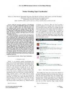
that, for low-coherence sources with spectral bandwidths on the order of tens of nanometers (i.e., coherence lengths on the order of tens of microns), the intensity noise term σ in2 = ρ 2 (1 + V 2 )( Pr + Px ) 2 B / Δν becomes dominant for reference powers greater than a few microwatts (see Figure 2.2). After this point Pr _ op , increasing the input source power does not improve the SNR since both the numerator and denominator in equation (2.4-13) increase at the same rate. For the case when the intensity noise is dominant, the SNR is proportional to Ps / Pr . Under these conditions, it can be seen that to improve the SNR and therefore the minimum reflection sensitivity, the reference power must be
21 selectively attenuated. Below this Pr _ op , the receiver noise σ re2 = 4k B TB / Reff dominates and SNR degrades as decreased Pr . The optimized value for the reference power Pr _ op occurs when the noise contributions due to the receiver and intensity are equal.
[29]
At
Pr _ op , however, the shot-noise limit SNR can hardly be reached in un-balanced detection.
0
S NR degradation: dB
-5
S hot noise limit
-10
-15
Receiver noise dominates
-20
Optimum reference power
-25
-30 -9 10
10
-8
10
-7
10
S ource intensity noise dominates
-6
10
-5
10
-4
10
-3
P ---ref: W atts
Figure 2.2. The effect of reference power on SNR degradation with respect to the shot noise limit for un-balanced OCT.
2.4-5 Noise feature and SNR of balanced OCT In balanced detection configuration, the excess source intensity noise is suppressed.
[15]
However, the balanced detection gives rise to another noise source,
named beat noise, which is given by [15]
22
σ be2 = 8 ρ 2 (1 + V 2 ) Pr Px B / Δν
(2.4-15)
For Px much less than Pr , the beat noise in equation (2.4-15) is much smaller than the intensity noise in equation (2.4-10).
In balanced detection configuration, since the receiver noise and shot noise are retained, the total photocurrent variance is then 2 σ bal = σ re2 + σ sh2 + σ be2
(2.4-16)
and the SNR is SNRbal =
8 ρ 2 Pr Ps 2 σ bal
=
4 K B TB / Reff
8 ρ 2 Pr Ps + 2eρ ( Pr + Px ) B + 8 ρ 2 (1 + V 2 ) Pr Px B / Δν
(2.4-17) It is easy to show that,
32 ρ 2 K B TBPS / Reff d ( SNRbal ) = >0 d ( Pr ) linear function of ( Pr )
(2.4-18)
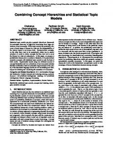
which indicates that SNR increases monotonically as reference power increases. However, SNR reaches a plateau or the shot-noise limit when reference power is above certain value (see Figure 2.3). Assuming the same values of ρ = 1 A / W , T = 300K ,
V = 0.5 , Δν = 1.05 × 10¹³ Hz and Reff = 100 KΩ as those of the un-balanced detection case in previous section, the SNR becomes a plateau when reference power reaches a saturation level of Pr _ sat ≈ 10 μW . Comparing with unbalanced OCT where SNR reaches its optimum at Pr _ op ≈ 1.2 μW and decreases above Pr _ op , balanced configurations
23 renders advantage on the true shot-noise limit detection and fully utilization of reference power.
0
S NR degradation: dB
-5
S hot noise limit
-10
-15
Receiver noise dominates
-20
S aturated reference power
-25
-30 -9 10
10
-8
10
-7
10
-6
10
-5
10
-4
10
-3
P ---ref: W atts
Figure 2.3. The effect of reference power on SNR degradation with respect to the shot noise limit for balanced OCT.
2.5 Velocity detection sensitivity in ODT As discussed in section 2.2, ODT is an extension of OCT such that localized Doppler flow imaging can be performed by using coherent detection to monitor moving scatterers within the sample. The interferometric fringe frequency detected in ODT arises from the net sum of phase modulation frequency f m generated by the reference beam and the additional Doppler shift f d by (potentially) moving scatteres in the sample. Coherent
24 (phase-sensitive) demodulation of the detector current at f m results in the complex envelope of the interferogram: [30]
~ iODT (t ) ≈ A(t ) exp[− j{2π f d t − φ (t )}]
(2.5-1)
where A(t ) , φ (t ) are the same as in equation (2.2-9): A(t ) is the amplitude of the sample reflectivity as a function of depth (time), and φ (t ) is a phase term dependent on the exact axial position of the scatterer and its intrinsic backscatter spectrum. Since each depth or A-scan is generated by time-delay scanning of the reference beam and is thus a time-domain signal, and Doppler shifts (i.e., spectral information) changes with depth, highly localized flow measurements are performed using joint-time-frequency analysis. [30]
Most commonly, the short-time Fourier transformation (STFT) is applied to the net
detector current (comprising the summation in equation (2.5-1) over all moving scatterers) for each depth scan, resulting power spectra corresponding to several “shorttime” sections of the A-scan. The local Doppler frequency generated by moving scatteres is estimated from the centroid of each spectrum and related to the mean velocity, υ s , of the scatteres by:
υs =
f d λ0 2n g cos θ
where n g is again the mean tissue index of refraction, and θ
(2.5-2)
is the Doppler angle
between the incident beam and direction of motion of scatterers within the sample.
2.5-1 Velocity resolution in ODT with STFT The velocity resolution, defined as the minimum resolvable velocity, υ smin , is directly proportional to the minimum detectable Doppler shift. Because detection of
25 Doppler shift using STFT requires sampling the interference fringe intensity over at least one oscillation cycle, the minimum detectable Doppler frequency shift, f dmin , varies inversely with STFT window size Δt (i.e., f dmin ≈ 1 / Δt ). [9] With a given STFT window size Δt = Nt s , where t s is the sampling interval, and N is the length of window in terms of t s , velocity resolution is given by
υ
min s
λ0 f dmin λ 0 1 = = 2n g cos θ 2n g cos θ Δt
(2.5-3)
The maximum resolvable velocity, υ smax , on the other hand, is set by the Nyquist rate as:
υ smax =
λ0
1 4n g cosθ t s
(2.5-4)
Besides the velocity resolution, the spatial resolution of ODT flow imaging is also determined by STFT window size and is given by [9] Δx = υ scan Δt
(2.5-5)
where υ scan is the one-dimensional depth scanning speed of the ODT system. Therefore, a large STFT window size increases velocity sensitivity while decreasing spatial resolution.
In ODT, there is yet another property, the image acquisition rate, or the frame rate, is important because of the blood flow monitoring objective of this technique. The frame rate, R f , is related to the velocity resolution by [30]
υ smin =
λ0
KLR F
2n g cos θ
ζ
(2.5-6)
26 where K is the number of A-scans per image, L is the number of pixels of velocity imaging in each A-scan, and ζ is the axial scanning duty cycle. Equation (2.5-6) suggests a compromise between the desired frame rate and the minimum dateable velocity.
2.5-2 Velocity resolution in ODT utilizing phase changes between sequential A-scans In STFT technique, since the Fourier transform is taken from single A-scan signal, the velocity resolution is limited by the relatively small window size. If the phase change during the sequential A-scans is used, which is equivalent to a much larger time window with STFT, a much better velocity sensitivity can be achieved. Denoting the period of an A-scan with T , the minimum detectable flow velocity is limited by the phase noise: [31]
υ smin ≥
λ0
1 φ noise 2n g cosθ T 360 o
(2.5-7)
where φ noise is a random noise term of the phase φ in equation (2.5-1) representing instabilities in the interferometer. The velocity sensitivity described in equation (2.5-7) could be significantly improved compared to that in equation (2.5-3) for a stable interferometer ( φ noise > Δt .
The maximum detectable flow velocity in this case is limited by the requirement that a moving scatterer must remain laterally within the focal region w0 of light beam and axially within the coherent length, l c , for at least T : [31]
27
υ smax ≤
l ⎤1 1 ⎡ w min ⎢ 0 , c ⎥ 2 ⎣ sin θ cosθ ⎦ T
(2.5-8)
Because T >> Δt , the maximum detectable flow velocity in equation (2.5-8) is much smaller than that in equation (2.5-4). This indicates that there is also a trade-off between velocity sensitivity and the up limit of the detectable velocity.
2.6 Summary In this chapter, a comprehensive review on the most important features of OCT and ODT is given. Principles of OCT and ODT are addressed at first; followed by discussions of OCT longitudinal and lateral imaging resolutions. For unbalanced and balanced OCT configurations, noises from primary sources are described and SNR properties of both setups are analyzed. It is found that at balanced OCT scheme, the SNR monotonically reaches shot-noise limit as the reference light power increases. The chapter is ended with the study on velocity detection properties and trade-offs present in ODT.
28
Topic I
Cancellation of Coherent Artifacts in Optical Coherence Tomography
Abstract: Low coherence sources generally experience slight modulation ripple on top of the principle spectrum. This modulation originates from residual multiple reflections inside the source; and when this source is implemented in coherent imaging such as in OCT, it gives rise to coherent artifacts. In this topic, we first discuss the cause of spectrum modulation and the coherent artifacts it generated using SLD as an example.
Coherent artifacts can severely degrade OCT image quality by introducing false targets if no targets are present at the artifacts locations.
These artifacts can add
constructively or destructively to the targets that are present at the artifact locations. This constructive or destructive interference will result in cancellation of the true targets or display of incorrect echo amplitudes of the targets. In this topic, we demonstrate that a non-linear deconvoluation algorithm, CLEAN, can be used to reduce coherent artifacts in OCT system. We have modified CLEAN and adapted it to a conventional OCT system, and have shown that the artifacts can be effectively reduced to background noise level. As a result of artifact reduction, the image contrast of the extracted tooth has been improved significantly.
CLEAN also sharpens the air-enamel and enamel-dentin
interfaces and improves the visibility of these interfaces which will be beneficial to diagnosis.
29 3. The Origination of Coherent Artifacts in Optical Coherence Tomography
3.1 Introduction OCT exploits the short temporal coherence of broadband light sources to achieve optical scanning of scattering tissue in depth dimension, and obtains multidimensional images of the tissue by adding spatial scanning.
[2, 32]
At each spatial location, the OCT
scanner output is the Fourier transform of the source spectrum convolved with the complex tissue reflectivity
[33]
and with the transfer function of the detection system.
Assume that the transfer function of the detection system is an ideal delta function, the OCT imaging outcome is then governed by the source property. It has been demonstrated in chapter 2 that the finite width of the source spectrum limits OCT longitudinal imaging resolution. Accordingly, the basic requirement of a source in OCT is with broad spectrum and sufficient output power to achieve high resolution and sensitivity. Among available sources superluminescent diode (SLD) is the most commonly used one,
[2]
while other
types such as erbium-doped fiber amplifier (EDFA) [34] and femotosecond pulsed laser [35] have also been employed. Practically however, none of the sources used has a perfect emission spectrum to form an idea image with resolution bounded in the sense of Rayleigh criterion. [18] It is well known that the spectrum imperfectness of the OCT low coherence sources stems primarily from the non-uniform gain/absorption properties of the active medium,
[36]
which shapes the source spectrum with dips and consequently
results in longitudinal resolution degradation.
[18]
Besides, there generally exists slight
modulation ripple on top of the principle spectrum. In this chapter we will demonstrate that this spectrum modulation originates from residual multiple reflections inside the
30 source; and when this source is implemented in coherent imaging, it gives rise to coherent artifacts. The source spectrum modulation by internal residual reflections has been less explored because it could be relatively weak compared with the principle spectrum, however, the generated coherent artifacts can not be neglected in OCT scanning when the light is reflected from a series of targets. [4, 34, 37, 38] Our discussion of the modulation and coherent artifacts generation will be on SLD simply because of its popularity in OCT setups; nevertheless, the addressed principle is applicable to other types of sources.
3.2 Physics of SLD Superluminescent diode (SLD), also called superluminescent LED (SLED), is a light-emitting diode in which there is stimulated emission with amplification but insufficient feedback for oscillations to build up to achieve lasing action.
[39]
SLD is
similar in geometry to laser diode (LD), but have no built-in optical feedback mechanism required by LD to achieve lasing of stimulated emission. SLD has structural feature similar to those of edge-emitting LED (ELED) that suppresses the lasing action by reducing the reflectivity of the facets. An SLD is, in essence, a combination of LD and ELED. [40] The functioning principles of LED, LD, and SLD are compared schematically in Figure 3.1.
An idealized LED emits incoherent spontaneous emission over a wide spectral range into a large solid angle. The un-amplified light emerges in one pass from a depth limited by the material absorption. The LED output is unpolarized and increases linearly
31 with input current. An idealized LD emits coherent stimulated emission (and negligible spontaneous emission) over a narrow spectral range and solid angle. The light emerges after many passes over an extended length with intermediate partial mirror reflections. The LD output is usually polarized and increases abruptly at a threshold current that provides just enough stimulated gain to overcome losses along the round-trip path and at the mirrors.
Figure 3.1. Schematic comparison of light-emitting diode, laser diode, and superluminescent diode in terms of amplification and feedback. (Modified from Ref. [41])
In an idealized SLD, however, the spontaneous emission experiences stimulated gain over an extended path and, possibly, one mirror reflection, but no feedback is provided. The output is low coherent compared with LD due to the spontaneous emission; on the other hand, it is high power with respect to LED because of the
32 stimulated gain. The SLD output, which may be polarized, increases superlinearly versus current with a knee occurring when a significant net positive gain is achieved. [42]
SLD is one of the semiconductor optical sources leading to substantial improvements in photonics. Because of its relatively high power at the order of mW and low temporal coherence at an order of 10μm, SLD has also seen extensive implementation in low coherence interferometry
[37]
[2]
and OCT techniques.
In order to
study the previously mentioned spectrum modulation and its effect on coherence imaging, a detailed discussion of SLD physics is necessary.
3.2-1 Threshold condition of semiconductor optical resonator Semiconductor optical resonator formed by a gain medium with two cleaved facets as the reflective boundaries is the fundamental unit of semiconductor optical devices including SLD. Consider a semiconductor optical resonator of length L shown in Figure 3.2. Taking into account the scattering and absorption of light as it propagates in the gain medium, to obtain a steady state with light emission, it is required that
I 0 = R1 R2 I 0 exp[2(Γg − α ) L] where R1 and R2 are the reflectivities of two facets respectively, Γ , g ,
(3.2-1)
α , and L are
the confinement factor, optical gain, total loss, and length of the active medium, respectively. Equation (3.2-1) simply implies that light repeats itself after a round trip in the gain medium. From equation (3.2-1), a threshold gain can be defined by
g th =
1 1 1 [α + ln( )] Γ 2 L R1 R2
(3.2-2)
33
Figure 3.2 Schematic of a semiconductor optical resonator formed by a gain medium with two facets as the reflective boundaries. R1 and R2 are the reflectivities of two facets, L is the length of the gain medium between two facets.
or for the case of R1 = R2 = R ,
g th =
1 1 1 [α + ln( )] Γ L R
(3.2-3)
It is based on the observation that the optical gain varies almost linearly with the injected carrier density
n and can be approximately written as [43] g = a ( n − n0 )
(3.2-4)
or for threshold gain
g th = a ( nth − n0 )
(3.2-5)
34 where the slope a is the gain coefficient and achieve transparency (i.e., g = 0 when the threshold carrier density
nth = n0 +
n0 is the injected carrier density required to
n = n0 ). Combine equations (3.2-3) and (3.2-5),
nth is given by
1 1 1 [α + ln( )] Γa L R
(3.2-6)
The threshold current density is given by [43]
J th = where
e
nth ed τ e (nth )
(3.2-7)
is the electron charge, d is the thickness of the active medium, and
τ e (n) = ( Anr + Bn + Cn2 ) −1
(3.2-8)
is the carrier-recombination time that is in general depends on n , where
Anr , B , C are
the nonradiative recombination rate, radiative recombination coefficient, and Auger recombination coefficient, respectively. [43] Since experimentally it is more convenient to measure the device current, an expression for calculating the threshold current can be given by
I th = J th Lw =
nth eLwd nth eV = τ e (nth ) τ e (nth )
where V = Lwd is the volume of the active layer, and the active layer, respectively. The typical values of
(3.2-9)
L , w are the length and width of
L , w , d , Γ , α , a , n0 , Anr , B ,
and C for a 1.3 μm buried-heterostructure [43] semiconductor optical device are shown in Table 3.1.
35 Table 3.1 Typical parameter values of a 1.3 μm buried-heterostructure semiconductor optical device
Parameter Resonator length Active-region width Active-layer thickness Confinement factor Loss Gain constant Carrier density at transparency
Symbol
n0
Value 250 μm 2 μm 0.2 μm 0.3 40 cm-1 2.5×10⁻¹⁶ cm2 1×1018 cm-3
Nonradiative recombination rate
Anr
1×10⁸ s-1
Radiative recombination coefficient Auger recombination coefficient
B
1×10⁻¹⁰ cm3/s
C
3×10-29 cm6/s
L
w d
Γ
α
a
Figure 3.3 Calculated threshold current as a function of facet reflectivity in two cases. One case is R1 = R2 = R , and I th reaches close to 220mA as the reflectivities of both facets reduce to 10-4. In the other case of R1 = 0.35 , I th reaches close to 150mA as R2 reduces to 10-4.
36 Based on the parameters taken from Table 3.1, the threshold current versus facet reflectivity is calculated in Figure 3.3. The result demonstrates that decreasing the facet reflectivities has the effect of increasing the threshold current, above which the device will be lasing. If the injection current is below the threshold current, the semiconductor optical device will work in the spontaneous emission mode since no osciliation can build up in the gain medium. At this mode, the output is the amplified broadband spontaneous emission. Figure 3.4 shows a typical emission spectrum at this mode. If the facet reflectivities is fabricated very low, the optical resonator can operate in spontaneous emission mode at very high injection current. Normally a cleaved facet of semiconductor optical device has a reflectivity abround 35%. [43] Techniquelly very low facet reflectivity can be made by three approaches: anti-reflection coating on normally cleaved facet,
Figure 3.4. Measured spontaneous emission spectrum of a commercial SLD (Optospeed SLED 1300-S5A D1-243).
37 buried facet, and tilted facet. At very low reflectivity, the high threshold current permits high output power without lasing, hence, making the device superluminescent while maintaining a broad spectrum.
3.2-2 Light-current characteristic of SLD A. SLD of only one facet antireflection-fabricated An SLD with one facet antireflection-fabricated is shown in Figure 3.5 (a). The total spontaneous emission rate per unit volume is defined as [43]
Rsp = β sp BnN = β sp Bn 2V
(3.2-10)
where β sp is the spontaneous-emission factor.
The equation describing the amplification of spontaneous emission in the +Z direction is given by [44]
dP+ = GP+ + βRsp dZ
(3.2-11)
where P+ denotes the photon number being amplified in the +Z direction, and β is the fraction of this radiation that is directed into the appropriate solid angle and gets amplified. The quantity G is the net gain given by G = Γg − α
(3.2-12)
From (3.2-12), with the boundary condition at Z = 0 to be P+ (0) = 0 , we get P+ ( L) =
βRsp G
(e GL − 1)
(3.2-13)
38
(a)
(b)
Figure 3.5 Schematic of the SLD. (a) One facet antireflection-fabricated, (b) Both facets antireflection-fabricated.
For the radiation traveling in the –Z direction, the equation is
dP− = −GP− + βRsp dZ
(3.2-14)
with the boundary condition at Z = L to be P− ( L) = RP+ ( L) . From equations (3.2-13) and (3.2-14) we have the following expression for the superluminescent output from the antireflection facet ( P1 ) and the non-antireflection facet ( P2 ): [44]
39
P1 = P− (0) =
βRsp G
(e GL − 1) (Re GL − 1)
P2 = (1 − R) P+ ( L) = (1 − R)
βRsp G
(e GL − 1)
(3.2-15)
(3.2-16)
B. SLD of both facets antireflection-fabricated We consider now an SLD with both facets antireflection-fabricated as shown in Figure 3.5(b). The equation describing the amplification of spontaneous emission in the +Z direction is again given by [45]
dP+ = GP+ + βRsp dZ
(3.2-17)
From (3.2-17), with the boundary condition at Z = 0 to be P+ (0) = 0 , we get P+ ( L) = P =
βRsp G
(e GL − 1)
(3.2-18)
and the power output from the other facet is P− (0) = P+ ( L) = P .
Similar to equation (3.2-7), generally the current density J is related to carrier density n by
J=
ned τ e (n)
(3.2-19)
and the current flow is
I = JLw
(3.2-20)
The use of equations (3.2-19), (3.2-20), and (3.2-8) leads to a third-degree polynomial of
n that can be used to obtain n as a function of the device current I
40
eVCn3 + eVBn 2 + eVAnr n − I = 0
(3.2-21)
After n is specified, the photon number P can be obtained using equations (3.2-4), (3.210), (3.2-11) and one of (3.2-15), (3.2-16), (3.2-18) for each facet of one facet antireflection SLD and both facets antireflection SLD, respectively. The output power is related to P linearly by P out =
1 hωυ g αP 2
(3.2-22)
where h is Plank constant, ω = 2πν is the angular frequency of the light, υ g = c 0 μ g is the group velocity of light in the active medium. A typical light-current characteristic of
(a)
(b)
Figure 3.6 Light-current characteristics of SLD source. (a) Calculated lightcurrent characteristics of SLD source for three output cases: (1) light output from the antireflection facet of one facet antireflection-fabricated SLD, (2) light output from the non-antireflection facet of one facet antireflection-fabricated SLD, (3) light output from each facet of both facets antireflection-fabricated SLD. (b) Measured light-current characteristics of a commercial SLD source.
41 SLD is shown in Figure 3.6 (a) by choosing parameter values of β sp = 5 × 10 −5 ,
β = 0.05 , μ g = 4 , and using Table 3.1. The calculation is for three cases: (1), one facet antireflection SLD, light output from the anti-reflection facet; (2), one facet antireflection SLD, light output from the non-antireflection facet; (3), both facets antireflection SLD, light output from both facets. The light-current characteristic of a commercial SLD source is measured as a comparison in Figure 3.6 (b).
3.3 The Fabry-Perot modes modulation of SLD spectrum If the spontaneous emission spectrum of SLD source in Figure 3.4 is displayed in high resolution, it reveals periodic ripple overlapping atop the spectrum envelope, as
Figure 3.7. The spontaneous emission spectrum modulation of a commercial SLD (the same as that in Figure 3.4). The spectrum analyzer is set at a resolution of 0.1nm.
42 shown in Figure 3.7. The appeared ripple is actually a modulation upon SLD spontaneous emission by Fabry-Perot modes. To achieve superluminescence, facet reflectivity of SLD has to be made very small; however, the residual facet reflectivity makes two facets to form a Fabry-Perot resonator naturally, resulting in the mode modulation of spontaneous emission spectrum.
3.3-1 Fabry-Perot mode spacing As shown in Figure 3.7, the Fabry-Perot modes are closely spaced (about 1.0nm). The mode spacing is determined by the optical resonator geometry and can be found through simple calculation. [15]
The wave-length λ and frequency ν of light is related as
ν=
By using equation
c
λ
=
c0
μgλ
(3.3-1)
Δν dν c ≈ = 2 , where c = c 0 μ g , the frequency difference between Δλ dλ λ
two modes can be approximated by: Δν =
c0 Δλ
μ g λ2
(3.3-2)
Because of the feedback in the resonator itself, only an integer amount of half wavelengths are contained within the diode. The number of these standing waves in the resonator can be written as
λ 2
m = Lμ g
(3.3-3)
43
where m is an integer. Rewriting this we get λ =
ν=
2 Lμ g m
=
c0 m 2 Lμ g2
c0
μ gν
or in terms of ν
(3.3-4)
The frequency spacing between two modes must then be Δν =
c0 c0 ( m − (m − 1)) = 2 2 Lμ g 2 Lμ g2
(3.3-5)
Since Δν in equations (3.3-2) and (3.3-5) must equal to each other, we have c0 c Δλ = 0 2 2 2 Lμ g μ g λ
(3.3-6)
Rewriting this gives Δλ =
λ2 2 Lμ g
(3.3-7)
For a 1.31μm SLD source with typical active region length L = 250 μm and group refractive index μ g = 3.5 , the Fabry-Perot mode spacing is expected to be 0.98nm, which is very close to the mode spacing measured in Figure 3.7.
3.3-2 The effect of facet reflectivity on modulation level In order to investigate the effect of facet reflectivity on the level of modulation ripple, a general Febry-Perot resonator is considered in terms of light filed propagation. As shown in Figure 3.8, the light filed incident on any facet is the integration of infinite field components resulting from multiple reflections. The total filed at facet, therefore, is the maximum when all of the field components are in phase with each other, that is
44 ∞
Fmax = F0 ∑ R n e n ( Γg −α ) L = n =0
F0 1 − R e ( Γg −α ) L
(3.3-8)
In equation (3.3-8), the simplification of the summation requires R e ( Γg −α ) L < 1 , which is satisfied for sub-threshold situation.
Figure 3.8 A general illustration of Febry-Perot resonator. Both facets have intensity reflectivity R , F0 is the light filed. Other parameters are referred to Figure 3.2.
Similarly, the total filed at facet is the minimum when all of the field components are out of phase with each other, that is ∞
Fmin = F0 ∑ (−1) n R n e n ( Γg −α ) L = n =0
F0 1 + R e ( Γg −α ) L
(3.3-9)
45 Denoting the maximum and minimum powers with I max and I min , we have
Fmax = (I max )1 / 2 and Fmin = (I min )1 / 2 . The ratio γ of the maximum to the minimum power in the spontaneous emission spectrum, or denoted as the modulation ripple level of the Fabry-Perot modes, is given by dividing equations (3.3-8) and (3.3-9): 2
⎡F ⎤ ⎡1 + R e ( Γg −α ) L ⎤ I γ = max = ⎢ max ⎥ = ⎢ ( Γg −α ) L ⎥ I min ⎣ Fmin ⎦ ⎣1 − R e ⎦
Figure
3.9
gives
one
example
of
γ
2
versus
(3.3-10)
facet
reflectivity
for
(Γg − α ) L = 0.001 . Since the SLD facets are anti-reflection fabricated, the spectrum
modulation ripple could be very small (less than 0.2dB in Figure 3.7). Nevertheless,
Figure 3.9 Spontaneous spectrum ripple γ as a function of facet reflectivity R at
(Γg − α ) L = 0.001 .
46 multiple-reflection inside optical cavity is not the only cause of spectrum modulation. Any defect in light delivery path will introduce multiple reflections, and if it happens to exist two defects forming a Febry-Perot resonator, additional modulation is produced.
3.4 Coherent artifacts generated by source spectrum modulation When a source spectrum is modulated at a level of
γ and a period of Δν , the
power spectrum density (PSD) can be expressed as
S (ν ) = S 0 (ν )(1 + γ cos
2πν ) Δν
(3.4-1)
where S 0 (ν ) is the ideal PSD when there is no modulation ripple. According to equation (2.3-4), the complex coherence function g (τ ) is the Fourier transform of source PSD S (ν ) . For a modulated PSD represented by equation (3.4-1), the important modulation
theorem of Fourier Transform indicates that, the corresponding complex coherence function g (τ ) should be expressed by g (τ ) = g 0 (τ ) +
γ ⎡
1 1 ⎤ g 0 (τ − ) + g 0 (τ + ) ⎢ 2⎣ Δν Δν ⎥⎦
(3.4-2)
where g 0 (τ ) is the complex coherence function corresponding to ideal PSD that is free of modulation. The right side of equation (3.4-2) indicate that there exist three coherence function terms when the source PSD is modulated at a level of
γ and a period of Δν .
Among those one is the principle coherence function g 0 (τ ) , and the other two are symmetric sidelobes located ± (1 Δν ) away from g 0 (τ ) , and the strength of the
47 sidelobes is
γ 2 of the principle coherence function. These sidelobes determines that
coherent artifacts are generated in OCT imaging.
3.5 Summary In this chapter the principle of a typical low coherence source, superluminescent diode, has been discussed in detail to demonstrate that the residual multiple reflections inside the source optical cavity introduces modulation to the PSD of the light output. This spectrum modulation generates sidelobes to the complex coherence function, which will appear as coherent artifacts in OCT imaging.
48 4. Cancellation of Coherent Artifacts using CLEAN algorithm
4.1 Introduction OCT scanner output is the Fourier transform of the source spectrum convolved with the tissue reflectivity over a narrow scattering angle and with the transfer function of the detection system. It has been discussed in the previous chapter that assuming the transfer function of the detection system is an ideal delta function, the imperfect Gaussian shape of source spectrum will introduce coherent artifacts or sidelobes. On the other hand, however, if the source spectrum is ideal, the non-ideal transfer function of detection system may introduce coherent spikes due to reflections from optical components, and these coherent spikes will present in OCT images as coherent artifacts. In a realistic OCT system, the coherent artifacts can be introduced by both sources. Several authors have reported coherent artifacts or coherent sidelobes observed in their OCT systems. 38]
[4, 34, 37,
These artifacts were primarily due to internal multiple reflections inside the source
which resulted in an imperfect source spectrum. The locations and strengths of these artifacts vary with the source and source current level as well as with the detection system configuration. Coherent artifacts can severely degrade OCT image quality by introducing false targets if no targets are present at the artifact locations. Artifacts can also add constructively or destructively to the targets that are present at the artifact locations. This constructive or destructive interference will result in cancellation of the true targets or display of incorrect echo amplitudes of the targets. In this chapter we demonstrate that these artifacts in OCT images can be effectively reduced to background noise level by using an iterative nonlinear deconvolution procedure known as CLEAN.
49 CLEAN was invented in the middle 1970s in radio astronomy modified later for use in microwave imaging.
[47]
[46]
and was
In ultrasound similar deconvolution
procedures were used to reduce the refractive artifacts. [48] In OCT the use of CLEAN to reduce speckle noise caused by interference of nonresolvable scatterers of highly scattering tissue has been reported by Schmitt.
[49]
In this reference, CLEAN has been
implemented using a theoretical point spread function with a Gaussian envelope. Therefore, the coherent artifacts due to imperfect Gaussian source spectrum or non-ideal detection optics have not been considered. In addition, the author has used a nonconventional OCT system with an array of sources and detectors, which enables CLEAN to be implemented in two dimensions.
In this chapter, we focus on the use of CLEAN, implemented in a conventional OCT system, to cancel coherent artifacts in OCT images of extracted teeth. A human tooth as illustrated in Figure 4.1 consists of a crown and root. The junction between the crown and the root is called the cervical margin. The tooth crown is covered by an acellular and highly mineralized tissue, the enamel. Enamel is translucent and varies in thickness from a maximum of 2.5 mm to a featheredge at the cervical margin. The bulk of the tooth is comprised of dentin. Dentin is a hard, elastic, avascular tissue that is approximately 70% mineralized. The interior of the tooth is called the pulp. The pulp consists of soft connective tissue that is innervated and highly vascular. In our work, we show that CLEAN reduces the artifacts associated with the air-enamel and enamel-dentin interferences to the noise floor, sharpens these interferences and improves the contrast between the interfaces and the surrounding medium.
50
Figure 4.1 Sketch of a sagittal section of human tooth.
4.2 Basic Principle 4.2-1 Point spread function The point spread function (PSF) of an OCT scanner depends on the coherence length of the source and the effective aperture defined by the pupil functions of the source and the detection optics. [49] Consequently, it is a two-dimensional (2-D) function and is denoted as h ( x , z ) , where z and x are the propagation and lateral dimensions, respectively. In conventional OCT scanners, a single beam is scanned across the sample, therefore the spatial distribution of h ( x , z ) can not be measured. Figure 4.2 illustrates the pertinent issue. A point scatterer is located in the medium and it scatters the incident light. The reflected light within a narrow angle is received by the detection optics and the off-axis scattered light falls outside of the receiving aperture. If more detectors were located at the off-axis positions, the scattered light could have been received over a larger
51 angle and the h ( x , z ) in x dimension could have been measured. However, since the incident beam is highly focused and the energy received over the beam spot area far exceeds the energy of off-axis scattered light, it is possible to use one-dimensional point spread function h( z ) ≈
∫ h( x, z )dx
to estimate the h ( x , z ) . We have found that
beam − spot − area
using this approximated PSF in CLEAN, a large portion of the sidelobe energy can be removed effectively.
Figure 4.2. A diagram of the conventional OCT scanning in the sample arm. The on-axis reflected light within a narrow angle is received by the detection optics, while the off-axis scattered light falls outside of the receiving aperture. If more detector fibers were located at off-axis positions (broken fiber lines), the scattered light over a wider angle could have been received.
52 4.2-2 Conventional deconvolution Assume that the medium contains N point scatterers each has complex strength of Cj. The original image that we wish to reconstruct is N
Oimage ( x, z ) = ∑ C jδ ( x − x j , z − z j )
(4.2-1)
j =1
where x j and z j are the coordinates of the j 'th scatterer. The "dirty" image is Dimage ( x, z ) = Oimage ( x , z ) ∗ h ( x, z ) + N ( x, z )
(4.2-2)
where ∗ denotes convolution and N ( x, z ) represents system noise.
Conventional deconvolution procedures perform Fourier transform on "dirty" image Dimage ( x , z ) and PSF h ( x , z ) to obtain their spatial frequency spectrum Dimage (u, v ) and h ( u, v ) . The original image can be recovered from the inverse Fourier
transform of
Dimage (u, v ) h ( u, v )
= Oimage (u, v ) +
N (u, v ) h ( u, v )
(4.2-3)
where Oimage (u, v ) and N (u, v ) are spatial frequency spectrum of Oimage ( x , z ) and N ( x, z ) , respectively. Unfortunately, this procedure is very sensitive to h ( x , z ) and the
system noise. In a practical OCT system, h ( u, v ) approaches zero rapidly due to limited bandwidth in axial direction and the effective aperture in the lateral direction. Therefore, this procedure is not robust and the deconvolution results depend highly on system noise. [49]
53 4.2-3 CLEAN procedure CLEAN provides more robust means to reconstruct the original image. CLEAN is performed in the spatial image domain and it iteratively recovers the original image. The basic steps of CLEAN algorithm are described as follows: First, find the brightest pixel [ x (1) , z (1) ] in the "dirty" image and subtract a fraction of the deconvolution kernel
αh[ x − x (1) , z − z (1) ]Dimage [ x (1) , z (1) ] / hmax
(4.2-4)
from the "dirty" image. The parameter α is called loop gain, which is less than unity, and it represents the fraction that is subtracted out by each iteration of CLEAN. Second, find the brightest pixel [ x ( 2 ) , z ( 2 ) ] from the residual of Dimage - αh[ x − x (1) , z − z (1) ]Dimage [ x (1) , z (1) ] / hmax
(4.2-5)
and repeat the first step. The iteration continues until the maximum value in the "dirty" image reaches the noise floor.
Assume that a total of M targets of strengths
αDimage [ x ( i ) , z ( i ) ] are found before iteration is stopped. The final CLEANed image is obtained by convolving the set of delta functions of strengths αDimage [ x ( i ) , z ( i ) ] at locations [ x ( i ) , z ( i ) ] with the clean beam of the point spread function containing only the mainlobe. Generally the residuals after CLEAN are added back to the CLEANed images to produce a realistic noise level in the final image.
4.2-4 1-D CLEAN procedure for conventional OCT imaging As discussed early, a 2-D PSF cannot be obtained from a conventional OCT scanner. Hence, we have used the 1-D PSF measured from a mirror to approximate the
54 2-D PSF. In this modified procedure, we first find the brightest pixel [ x (1) , z (1) ] in the “dirty” B-scan image and subtract a fraction of the deconvolution kernel
αh[ z − z (1) ]Dimage [ x (1) , z (1) ] / hmax
(4.2-6)
from the “dirty” A-scan line. We then, find the brightest pixel [ x ( 2 ) , z ( 2 ) ] from the residual of Dimage - αh[ z − z (1) ]Dimage [ x (1) , z (1) ] / hmax
(4.2-7)
and repeat the first step. The final CLEANed image is obtained by convolving the set of delta functions of strengths αDimage [ x ( i ) , z ( i ) ] at locations [ x ( i ) , z ( i ) ] with the clean beam of the 1-D PSF containing only the mainlobe. The disadvantage of using 1-D CLEAN is that the off-axis sidelobe energy is not removed. However, we have found that the offaxis sidelobe energy is significantly smaller compared with the on-axis sidelobe energy and 1-D CLEAN effectively reduces the sidelobe energy to the noise floor in the images.
4.3 Methods The schematic diagram of our OCT system is shown in Figure 4.3. The erbium-doped fiber amplifier (EDFA) at a center wavelength of 1550 nm is used as the low coherence source. The optical power output and 3dB coherence length of this EDFA at 40mA current are 0.43mW and 25μm, respectively. The light from the source enters the optical circulator (OC), and it split into a reference for the differential receiver input and a signal, which is passed through a 3 dB fiber coupler (FC), where the outputs form a Michelson interferometer. The reference arm of interferometer consists of a microscope objective (O1), a plane mirror, a speaker and a linear DC motor. The mirror is glued on
55 the bowl of the speaker, which is mounted on the linear motor. The speaker is used to provide phase modulation frequency and is driven by a sinusoidal wave of with a frequency of 100 Hz and peak-to-peak amplitude of 6.2 volts. The generated phase modulation is broadband and has a maximum of 17KHz. The depth (Z direction) scan is achieved by translating the speaker and motor assembly. The sample arm consists of a microscope objective (O2), a galvanometer scanner, a lens, and a sample. The alignment requirement for the sample arm is that not only the incident light is perpendicular to the rotation axis of the galvanometer mirror, but also the incident light spot is located at the focal point of the lens. With this precise alignment, the spatial (X direction) scanning is achieved by converting the rotation of the galvanometer mirror to a linear scanning upon the sample without introducing any change in optical path length.
Figure 4.3. Schematic diagram of the OCT system. EDFA, erbium-doped fiber amplifier; OC, optical circulator; FC, fiber coupler; O1, O2, microscope
56 objectives. G, galvanometer; L, lens. The galvanometer and linear motor are controlled by PC.
The data acquisition consists of a dual balanced optical receiver, a high pass filter and a PC. The interferometer output is detected by the dual balanced receiver, which is designed to reduce common-mode noise. The resulting signal is passed through a high pass filter for rejecting DC noise and preserving the broadband interference signals. We have found that a high pass filter tracks the peak Doppler frequency better than a band pass filter for this setup. The filtered signal is then sampled by an A/D converter at a sampling frequency of 400kHz, and the sampled data are Hilbert transformed to obtain the signal envelopes which forms An A-scan line.
The galvanometer and the linear motor are synchronized by the PC control software. A 10 Hz sine wave generated by the PC is used to drive the galvanometer controller, which in turn drives the scanning mirror. One set of B-scan data is acquired in 128 cycles of galvanometer rotation and 3.84 mm depth scanning of the reference arm. For the images presented, the transversal scanning range is set to 6 mm, and a total of 400 pixels are used. Thus the pixel size at transversal direction (X) is 15μm, which is less than 3dB spot size (~30μm) of the sample beam. The pixel size in depth direction (Z) is 15 μm, which is less than the free space image resolution of 25μm for EDFA source at 40mA driving current.
4.4 Results 4.4-1 System point spread function
57 The measured point spread function of the system is shown in Figure 4.4 (a). The
1
Main lobe
0.9
1
1
2
2
0.6
Side lobe
0.5
Side lobe
X (mm)
0.7
X (mm)
0.8
3
3
0.4
4
4
5
5
0.3 0.2
0.1
6
0 0
1
2
3
Z (mm)
6
1
2
3
2
3
Z (mm)
Z (mm)
(a)
1
(b)
(c)
Figure 4.4. The point spread function of the system and the resulting image artifacts. (a) Normalized point spread function of the system or A-scan line measured from a planar mirror. The horizantal axis is the propagation depth and the distance between the main lobe and the sidelobe is 1.335 mm. (b) Image of a mirror. The light propragation direction is from left to right. Vertical axis is the spatial scan dimension. The central line is the mirror, and the two lines at both sides of the central line are sidelobe artifacts. (c) Image of an extracted tooth. The central curve is the air-enamel interface. The sidelobe artifacts are clearly shown by two complicated curves, pointed out by the two vertical arrows, on both sides of the central curve.
58 distance between the mainlobe and the artifact positions is 1.335mm, which is within the 3.84 mm scan range. When a planar mirror is imaged, the artifacts create two parallel lines on both sides of the central image line (see Figure 4.4 (b)). Under this ideal imaging scenario, the artifacts can be easily identified. However, when the imaging medium is changed to an extracted tooth, the artifacts appear as two complicated curves on both sides of the air-enamel interface (see Figure 4.4 (c)). These artifact curves can be confused with real interfaces in diagnosis. Furthermore, if the enamel-dentin interface were located at the neighborhood of the artifact curve, it would not be imaged with correct echo amplitude.
4.4-2 CLEAN example 1 Figure 4.5 shows the “dirty” image of the extracted tooth (a) and the CLEANed image (b). Figure 4.5 (c) is the microscopic picture of the sectioned tooth imaged. The scanned region contained a fissure defect in the enamel (pointed by the black arrow in (c)). Diagnostically, it is important to determine whether or not such a defect extends beyond the enamel layer. Comparing OCT images before and after CLEAN, we can observe significant improvement in image detail in the fissure region (pointed by the arrow in the upper part of (a)). In addition, the two artifact curves on both side of the airenamel interface shown in Figure 4.5(a) are reduced to background level after CLEAN. The contrast between the air and the enamel has been improved and the interface is delineated well after CLEAN. Furthermore, the artifacts associated with the enamel-
59 dentin interface (pointed by the right arrow at the bottom of (a)) are removed and this
1
1
2
2 X (mm)
X (mm)
interface (pointed by the left arrow at the bottom of (a)) is enhanced after CLEAN.
3
3
4
4
5
5
6
1
2 Z (mm)
3
(a)
6
1
2 Z (mm)
(b)
3
(c)
Figure 4.5. CLEAN example 1. (a) Original tooth image. (b) CLEANed image. (c) Microscopic picture of the sectioned tooth imaged. The OCT image dimension is 6 mm (vertical, X) by 3.84 mm (horizontal, Z), the pixel size is 15 x15 μm2 . The sidelobe artifact curves are reduced to the background level. The air-enamel interface is enhanced after CLEAN, and the sidelobe energy of the enamel-dentin inference, pointed by the smaller arrow at the bottom right is removed after CLEAN.
60 To quantitatively assess the sidelobe artifact reduction, we show an A-scan line in Figure 4.6(a), which is obtained at Figure 4.5 (a) where there exist the air-enamel and enamel-dentin interfaces as well as the coherent sidelobes. The measured peak artifacts airairaiairair 0
-5
sidelobes of air-
enamel-dentin
sidelobes of airenamel and
enamel and
enamel-dentin
enamel-dentin
interfaces
interfaces
air-enamel
-10
-15
-20
-25 0
0.5
1
1.5
2
2.5
3
3.5
4
z (mm)
(a) 0
-5
-10
-15
-20
-25 0
0.5
1
1.5
2 z(mm)
2.5
3
3.5
4
(b)
61 Figure 4.6. Normalized A-scan lines (dB) from the “dirty “ image (a) and the CLEANed image (b). The A-scan position is shown in Figure 5(a). After CLEAN, the sidelobes associated with air-enamel and enamel-dentin interfaces are reduced to background noise level.
associated with these interfaces are –15 dB and are reduced to the background noise level after CLEAN (Figure 4.6(b)), and both interfaces are enhanced.
1
1
2
2 X (mm)
X (mm)
4.4-3 CLEAN example 2
3
3
4
4
5
5
6
1
2 Z (mm)
(a)
3
6
1
2 Z (mm)
(b)
3
(c)
Figure 4.7. CLEAN example 2. (a) Image of tooth with a metalic filling at the surface. (b) CLEANed image. (c) Microscopic picture of the sectioned tooth. The spatial scan range is indicated by the two arrows in (c). The portion of the air-enamel interface that is delineared well after CLEAN is pointed by the arrow at the top of (b). The indented portion of the air-enamel interface corresponds to
62 a cavity and is pointed by the longer arrow at the bottom of (b). The boundary and the internal aspects of the metallic restoration (within the frame) is visualized better after CLEAN.
Another example is shown in Figure 4.7 and a tooth that contained a metallic restoration is imaged. Diagnostically, it is important to verify smooth adaptation of the restoration to the tooth surface and to detect structural defects of the tooth at the interface. A noticeable improvement after CLEAN is the contrast between the restoration and the enamel. Since the metallic restoration has higher reflectivity than the tooth, the incident light is reflected at the air-restoration interface and the interior of the restoration should appear dark. However, the contrast between the restoration and the enamel is poor in the ‘dirty’ image because of significant artifact energy in the restoration. After CLEAN, the restoration-tooth interface is better visualized both at the surface and along the internal aspects of the restoration. In addition, the portion of the air-enamel interface, pointed by the bigger arrow at the top of the CLEANed image, is blurred and diffused in the background level in the ‘dirty’ image and is clearly visible after CLEAN. Another noticeable improvement is the boundary of a cavity at the tooth surface, pointed by the smaller arrow at the bottom of the CLEANEed image, and it is delineated well after CLEAN.
The residual artifact level after CLEAN is visible at several spatial locations. Since the reflectivity of the metallic restoration is strong, the signals returned from airmetal interface are saturated at several spatial positions and the extent of the saturation depends on the angle of incident light with the metallic restoration surface. As a result, the ratios of the peak artifact to mainlobe strength at these spatial positions are several
63 decibels higher than the ratio obtained from the mirror. Therefore, the artifact subtraction at these A-scan positions is not as complete as that obtained at the non-saturation positions, and it leaves larger residual artifact energy.
4.5 Discussion The strengths and positions of coherent artifacts caused by the imperfect source spectrum change with sources and the source current levels used. In Ref. [34], we have reported that the coherent sidelobe level increases with the source current when an erbium-doped fiber amplifier is used as a source. In Ref. [4], the authors reported that as the injection current increased, the gain of the diode was increased, and multiple internal reflections occurred which resulted in sidelobe level increase. Figure 4.8(a) and (b) show the measured source spectrum of the EDFA used in our system. As shown in the figures, the source spectrum has periodical ripple overlapped on top of the principle spectrum pattern. The interval between two ripple peaks is approximately 1nm, which in spatial domain corresponds to 1.29 mm. This distance is very close to the measured sidelobe position of 1.335 mm. Figure 4.8(c) is the Fourier Transform of the source spectrum shown in Figure 4.8(a), and it is the autocorrelation function of the source. The peak sidelobe level is about –27 dB. Since the measured PSF from a planar mirror (Figure 4.4(a)) is the convolution of the Fourier transform of the source spectrum with the transfer function of the detection system, the measured sidelobe positions and strengths are modified by the detection optics.
64
-29
-30
-30
dB
dB
-20
-40
-50
-31
-32
-60 1500
1520
1540
1560
1580
-33 1540
1600
1545
1550
(a)
1555
(b)
0 -10 -20
dB
-30 -40 -50 -60 -70 -80
0
1
2
3 Z (mm)
4
5
6
(c) Figure 4.8. Recorded optical spectrum of EDFA used in our OCT setup. (a) wavelength range is 1500-1600nm; (b) wavelength range is 1545-1565nm. The period of the ripples on top of the principle spectrum pattern is about 1 nm; (c) Fourier Transform of Figure 8(a) and it is the autocorrelation function of the EDFA source.
1560
65 There are many system parameters that the detection optics can modify the PSF. We have found that the reflectivity of the mirror used in the reference arm is an important parameter to affect the artifact strength. The thickness of the mirror used in the reported experiments was 1.0 mm and a few percent reflection from the back plate of the mirror produced a coherent spike which was located approximately at the source sidelobe position (1.0 mm x 1.33 (reflective index) = 1.33 mm). As a result, the measured artifact strength of our system PSF was higher than the sidelobe strength calculated from the autocorrelation function of the source spectrum. However, the results that CLEAN can reduce artifact level to noise background and improve image contrast are independent from artifact strength.
In this work, CLEAN is applied to A-scan data obtained from a conventional OCT scanner. Therefore, the CLEANed images still contain a small residual sidelobe energy caused by off-axis scattered light. Another factor that could affect the complete elimination of sidelobe artifacts would be the nonlinearity introduced by the scanning optics. Since the beam is scanned across the lens at the sample arm by a galvanometer (see Figure 4.3), the center beam alignment and the beam spot size vary with the galvanometer rotation angle. Therefore, slight spatial nonlinearity is introduced in the image.
Since this non-linearity also exists in the mirror image, we have used the
corresponding PSF measured at every spatial location to clean the extracted teeth images. However, we did not observe any visible changes in CLEANed images by using a single PSF and the corresponding PSF obtained at each spatial location.
66 In this work, CLEAN is applied to A-scan data, which is the envelop of the received A-scan signal. CLEAN can also be applied to the complex data, and the algorithm will be more powerful in recovering targets distorted by constructive and destructive interference caused by coherent artifacts. This subject requires further study.
The final image quality after CLEAN is affected by the stopping criteria. Since the signals cannot be distinguished if their levels are below the noise floor in the image, it is straightforward to choose the background noise level in the image as a stopping criteria when CLEAN is used. The final image quality is determined by the loop gain too. Tested with different loop gains of 1, 0.5, 0.25, 0.1, 0.05, 0.025 and 0.01, it is shown that there is distinguishable image quality change for loop gains of 1, 0.5, 0.25 and 0.1, but if loop gain is further reduced, no distinguishable image quality change is observed. In terms of processing time, using Pentium III 800MHz CPU, the computing times for loop gains of 1, 0.5, 0.25, 0.1, 0.05, 0.025 and 0.01 are all about 11 minutes. In our regular CLEAN, therefore, we choose 0.1 as the loop gain and the background noise level as the stopping criteria.
4.6 Conclusions Imperfect source spectrum and non-ideal detection optics in OCT system could introduce coherent artifacts. Coherent artifacts can severely degrade OCT image quality. In this chapter, we have demonstrated that a non-linear deconvoluation algorithm,
67 CLEAN, can be used to reduce coherent artifacts. We have modified CLEAN and adapted it to a conventional OCT system, and have shown that the artifacts can be effectively reduced to background noise level. As a result of artifact reduction, the image contrast of the extracted tooth has been improved significantly. CLEAN also sharpens the air-enamel and enamel-dentin interfaces and improves the visibility of these interfaces which will be beneficial to diagnosis.
68
Topic II
Optical Coherence Tomography System Modifications
Abstract: In this topic, we discuss the upgrading of our OCT system. A rapid scanning optical delay line based on Littrow-mounting of diffraction grating is introduced. It has been demonstrated that for balanced detection OCT setup, using this Littrow-mounting setup, the reference arm light power has minimum loss among grating-based delay lines, and the resulting SNR improvement is about 3dB.
Examples on imaging and diagnosis of nail fungal infection are also given as a demonstration of the imaging capability of this updated OCT system.
69 5. Optical Coherence Tomography System Based on A Scanning Optical Delay Line Configured with Littrow-mounting of Diffraction Grating
5.1 Introduction The OCT system described in previous topic is however, a prototype that performs relatively slow speed, less sensitivity and coarse resolution. It is well known that the axial resolution is a matter of coherence property of the light source; nevertheless, the configuration of optics determines other system parameters. In order to improve imaging quality such that certain OCT applications and ODT can be studied, we constructed a new OCT system. The modifications include a novel grating-based scanning delay line in the reference arm, a gradient index (GRIN) lens in the sample arm, a digitally programmable band-pass filter, and a commercial SLD source with superior spectrum. Because the advantages of implementing a better low coherence source, a GRIN lens and a high-quality filter are obvious, we will focus only on the reference arm modification. In this chapter, first we will review the fundamental electromagnetic theory of grating, and then discuss the principle and performance of a novel scanning delay line setup based on Littrow-mounting of diffraction grating.
5.2 A review on the fundamental electromagnetic theory of grating [50] A diffraction grating is an optical component used to disperse light. [51] It consists of a one-dimensional periodic array of similar apertures separated by a distance comparable to the wavelength of light under study. The periodically displaced apertures act as diffracting elements, therefore, an electromagnetic wave incident on a grating will,
70 upon diffraction, has its electric field amplitude, or phase, or both, modified in a predictable manner. [52, 53]
In our review of grating theory (which is digested from a rigorous and complete study of grating theory in Ref. 50), a rectangular coordinate system is preferred, where →
→
→
aˆ x , aˆ y , and aˆ z are denoted as the unit vectors of OX , OY and OZ (Figure 5.1). A → r point M is located by the vector r = OM whose components are x , y , and z . Only
time-harmonic electromagnetic fields with pulsatance ω is studied. Consequently any r r vector function a ( r , t ) is systematically represented by its associated complex vector
r r − iω t function A( r ) assuming a time dependence in e
a(r , t ) = ℜe[ A(r )e − iω t ]
(5.2-1)
Figure 5.1 The rectangular coordinate system used.
Since the resolving power is not to be discussed here, a grating is always assumed to be infinitely wide and is represented by a cylindrical surface y = f (x) whose
71 generatrices are parallel to the z axis (Figure 5.2). f (x ) Is a periodic function and its period d is the grating period, also called “grating spacing”. k = 2π / d Is then the associated grating wavenumber. The graph of f (x ) is a curve p which describes the grating profile. Let us call n1 the index of the homogenous and isotropic material which lies above p in region 1 [ y > f (x) ]; n1 is supposed to be real and very often is equal to unity. On the other hand, the index n2 of region 2 [ y < f (x) ] is either real (for transmission dielectric gratings) or complex (for conducting gratings or lossy dielectric gratings). If region 2 is filled with a perfectly conducting metal, n2 is meaningless, and a perfectly conducting grating is spoken of in this case.
Figure 5.2 Geometry of a grating profile and diffraction by a grating. By convention, angles of incidence and diffraction are measured from the grating normal to the beam. Here the incidence angle θ and the diffraction angle θ n are defined in such a way that they are both
OD = d , OA = a , c > a
positive.
OC = c ,
5.2-1 The perfectly conducting grating For simplification, suppose a perfectly conducting grating is illuminated under the incidence θ by a plane wave of unit amplitude propagating in region 1 (Figure 5.2). The r incident wave vector k i = k1uˆ lies in the xy plane; consequently the electromagnetic
72 field is non-dependent upon z .
r The components of k i upon x, y, z axes are,
respectively, α , − β and γ with
α = k1 sin θ i , β = k1 cosθ i , γ = 0
(5.2-2)
Two fundamental cases of polarization, namely P polarization or S polarization, are considered here. In P polarization the electrical vector field is parallel to the grooves r r r ( E = E z zˆ ) and it can also be called E || polarization. In S polarization, also called H || r polarization, it is the magnetic filed which is parallel to the grooves ( H = H z zˆ ). A
function u ( x, y ) , which is defined as E z in P polarization or H z in S polarization, will be used in order to treat the two polarization cases simultaneously. This function u ( x, y ) , whether it is E z in P polarization or H z in S polarization, is equal to zero in region 2 [ y < f (x) ], and, satisfies scalar Helmholtz Equation in region 1: Δu + k12 u = 0 , if y > f (x)
(5.2-3)
Moreover u ( x, y ) must satisfy a boundary condition. Normally the boundary condition r r r r r for E is n21 × ( E1 − E 2 ) = 0 , where n21 is the normal unit vector pointing from medium 2 r to medium 1. For the perfectly conducting grating, because E is null in region 2, we
have r r n21 × E1 = 0
(5.2-4)
r In P polarization, E = uzˆ and equation (5.2-4) implies Lim[u ( p)] = 0
Q→M
(5.2-5)
73 where Q designates a point located in region 1 and M is a point on the grating surface. Here we recognize a Dirichlet boundary condition which we can write more simply u[ x, f ( x )] = 0
(5.2-6)
r r In S polarization, H = uzˆ and E can be expressed in terms of u in region 1 r 1 1 E= ∇ × (uzˆ ) = grad u × zˆ iωε 1 iωε 1
(5.2-7)
Then the boundary condition equation (5.2-4) becomes
r n21 × Lim grad[u (Q)] × zˆ = 0 Q→M
(5.2-8)
r r r r r r r r r or, using the double vector product formula A × ( B × C ) = ( A • C ) B − ( A • B )C
r n21 • Lim grad [u (Q)] = 0 Q→ M
(5.2-9)
We also recognize a Newmann boundary condition which can be written using the normal derivative 1 du =0 dn y = f ( x)
(5.2-10)
The superscript 1 in equation (5.2-10) is used to recall that this normal derivative must be evaluated in region 1.
5.2-2 The diffracted field The total filed u in region 1 is the sum of the incident field and the diffracted field. Therefore, it is straightforward to define the diffracted field as the difference between the total field u and the incident field u i = exp[i (αx − βy )]
74 def
ud = u − ui
(5.2-11)
It is worth noting that u d , defined in this way, has no physical significance in region 2; on the other hand, it will be the unknown function in region 1. As for the incident field u i , which is a plane wave, verifies everywhere the Helmholtz Equation. Consequently,
starting from equation (5.2-3) and taking into account that the linearity of the Δ operator, we have that Δu d + k12 u d = 0 , for y > f (x)
(5.2-12)
From equations (5.2-6), (5.2-10), and (5.2-11), it turns out that u d verifies one or the other of the following boundary conditions: In P polarization:
u d [ x, f ( x)] = −u i [ x, f ( x)]
(5.2-13)
In S polarization:
1 1 du d du i =− dn y = f ( x) dn y = f ( x)
(5.2-14)
Moreover, physically it is leading to add a radiation condition: the assumption that, when y tends to infinity, u d must be bounded and described as a superposition of outgoing plane waves (such a radiation condition does not hold of course for the total field u because u i is an incoming plane wave).
Finally, the problem faced here, which can be called the grating problem, is to find a function which verifies the Helmholtz Equation (5.2-12), a boundary condition [in P equation (5.2-13) or in S equation (5.2-14) depending on the polarization] and the outgoing wave condition, or the radiation condition.
75 To find the solution of the grating problem, define a new function w( x, y ) as def
w( x, y ) = u d ( x + d , y ) exp(−iα d )
(5.2-15)
It is obvious that w( x, y ) satisfies the Helmholtz equation and the radiation condition as long as they hold for
u d ( x, y ) . Regarding the boundary condition, since
u i = exp[i (αx − βy )] has the property of u i ( x + d , y ) = u i ( x, y ) exp(iα d )
(5.2-16)
therefore, w( x, y ) satisfies the boundary condition. In P polarization, for example,
w[ x, f ( x)] = u d [ x + d , f ( x)] exp(−iα d ) = −u i [ x + d , f ( x)] exp(−iα d ) = −u i [ x, f ( x)]
(5.2-17)
In summary, w( x, y ) satisfies the Helmholtz equation, the boundary condition and the radiation condition. As a consequence of uniqueness theorem, we have then def
w( x, y ) = u d ( x + d , y ) exp(−iα d ) = u d ( x, y )
(5.2-18)
u d ( x + d , y ) exp[−iα ( x + d )] = u d ( x, y ) exp(−iαx)
(5.2-19)
or equivalently
Define another function v ( x, y ) as def
v( x, y ) = u d ( x, y ) exp(−iα x) ,
(5.2-20)
it can be seen from equation (5.2-19) that v ( x, y ) is a periodic function of period d with respect to x , i.e., that is, v ( x + d , y ) = v ( x, y )
(5.2-21)
76 Equation (5.2-20) yields that u d ( x, y ) = v( x, y ) exp(iα x)
(5.2-22)
which shows that u d ( x, y ) is the product of exp(iα x ) with a periodic function v ( x, y ) , and thereafter u d ( x, y ) could be called a pseudo-periodic function.
5.2-3 The Rayleigh expansion and the grating formula The periodic function v ( x, y ) can be represented by a Fourier series; then +∞
+∞
m = −∞
m = −∞
u ( x, y ) = exp(iαx) ∑ v m ( y ) exp(imkx ) = ∑ v m ( y ) exp(iα m x) d
(5.2-23) with
α m = α + mk = k1 sin θ i + mk
(5.2-24)
Let a be the maximum value of f (x ) . If y > a , u d ( x, y ) verifies the Helmoholtz Equation for any x . Substituting equation (5.2-23) to the Helmholtz Equation, it results that
⎡ d 2 vm ⎤ 2 2 ∑ ⎢ 2 + (k1 − α m )v m ⎥ exp(imkx) =0 m = −∞ ⎣ dy ⎦ +∞
(5.2-25)
The left-hand side can be looked upon as the Fourier serious of the null function, which implies that, for any value of the integer m d 2 vm + Ω m vm = 0 dy 2
(5.2-26)
Ω m = k12 − α m2
(5.2-27)
with
77
U being the set of integers for which Ω m is positive, let β m defined by ⎧Ω1m/ 2 1/ 2 ⎩ ( −Ω m )
βm = ⎨
if if
m ∈U m ∉U
(5.2-28)
Then, the general solution of equation (5.2-26) is v m ( y ) = Am exp(−iβ m y ) + Bm exp(iβ m y )
(5.2-29)
The radiation condition leads to Am = 0 because Am exp(imkx − iβ m y ) would represent an incoming wave for m ∈ U and would not be bounded for m ∉ U . Finally, from equations (5.2-23) and (5.2-29), we get an expansion of the diffracted field in terms of plane waves u d ( x, y ) =
+∞
+∞
m = −∞
m = −∞
∑ Bm exp(iα m x + iβ m y ) = ∑ Bmψ m ( x, y )
(5.2-30)
This equation is the Rayleigh expansion of u d ( x, y ) . In fact, each term of this expansion represents a propagating plane wave only if m ∈ U ; if m is sufficiently large, m ∉ U and the associated term represents an evanescent wave Bm exp(− β m y ) exp(iα m x ) which propagates along the OX axis and which is exponentially damped with respect to y . For the propagating waves, the diffracted wave in the m th order, is described by
ψ m ( x, y ) = Bm exp[iα m x + i (k12 − α m2 )
1/ 2
But, because
αm
y]
(5.2-31)
is less than unity, we can put
k1
αm k1
= sin θ md = sin θ i +
mk π π , − < θm < k1 2 2
(5.2-32)
Then
(k
2 1
− α m2 )
1/ 2
= k1 cos θ md
(5.2-33)
78 and equation (5.2-31) becomes
ψ m ( x, y ) = Bm exp[ik1 ( x sin θ md + y cos θ md )]
(5.2-34)
which proves that θ md is the angle of diffraction. As for equation (5.2-32), it is the wellknown grating formula, which is more frequently written in either of the two following forms: sin θ md = sin θ i + m
λ
(5.2-35)
d
or k1 sin θ md = k1 sin θ i + mk
(5.2-36)
Equation (5.2-35) explains the useful geometrical construction shown in Figure 5.3. Equation (5.2-36) can be explained that, in projection on the x axis, one passes from the incident wave vector to n th diffracted wave vector by adding n times the grating wavenumber k .
Figure 5.3. Graphic explanation of grating formula. The wavelength in region 1 is simply λ0 . The
r
incident wave vector k i cuts the circle of unit radius in I 0 . If
A0 An = m
λ0 d
, the m th diffracted
plane wave is propagating along
OJ md .
79 The complex coefficients Bm in equation (5.2-33) are closely related to efficiencies em . Consider (see Figure 5.2) the rectangle BCC ′B′ whose side CC ′ , of unit length, is parallel to the z axis. Let φ i and φ md represent the flux, through this rectangle, of the Poynting vector associated with the incident wave and the m th diffracted wave. Define em as
φ md , then we find that φi em = Bm Bm∗
cosθ md cosθ i
(5.2-37)
5.2-4 The Littrow mounting In usual mounting, there is a certain value of m for which the m th diffracted wave and the incident wave are propagating in opposite directions. As is shown by the geometrical construction (Figure 5.3) that can happen only with a negative value of m and we have 2 sin θ Li = − m
λ d
(5.2-38)
where the incident angle θ Li is called Littrow angle.
5.3 OCT system constructed with a scanning optical delay line based on Littrowmounting of diffraction grating OCT is capable of detecting light backscattered from a sample object with micrometer-scale resolution and high sensitivity. The principle of OCT relies on the interference of low-coherence light in a typically Michelson interferometer. One arm of the interferometer leads to the sample of interest, and the other leads to a reference
80 mirror. The detected interference signal is in general subject to source intensity noise. One way of minimizing source intensity noise is to attenuate the reference power properly. The alternate method proven to be more efficient is using balanced detection technique. [27] According to the discussion in chapter 2, the SNR of an OCT system under a balanced detection scheme is proportional to the product of detected powers of the reference arm and sample arm and is inversely proportional to the bandwidth of the detection electronics. It was shown that SNR increases monotonically as reference power increases before SNR reaches the shot-noise limit. A high SNR is necessary for detection of the extremely low light intensities backscattered from turbid samples. Moreover, for optical Doppler tomography application, the broadband detection causes SNR degradation, and higher optical power delivery is required to maintain SNR. This implies that the reference arm power should be preserved as much as possible so as to achieve highest available SNR for a given system.
In OCT, grating-based rapid scanning optical delay (RSOD) line that utilizes group-dispersion and phase-ramp to perform optical ranging has been implemented. [54, 55] This conventional grating-based RSOD is a modification of femotosecond Fouriertransform pulse shaping technique,
[56]
where a diffraction grating and a dithering plane
mirror placed at the Fourier planes of a lens are used to generate a linear phase-ramp resulting a group optical delay. This grating-based RSOD configuration has shown to be superior to most of other optical delay techniques for its flexibility, high speed, high duty cycle, phase- and group-delay independence, etc. Nevertheless, as long as a diffraction grating is used for taking advantage of dispersion, light is always diffracted into a
81 minimum of two orders (0th order, equivalent to simple reflection, and 1st order), in which the optical power in the 0th order is inevitably lost. Although the diffracted light energy can be concentrated into a specific order by the “blazing” of grating, a perfect blazing can never be achieved due to a finitely thin conducting deposition layer, absorption losses, and diffuse scatter, etc. An absolute efficiency of 70% is typical for blazed grating optimized in NIR range. When a dithering plane mirror is introduced in the distal end of reference arm to perform scanning optical delay, the light experience diffraction one more time, and the optical power loss by diffraction is at least doubled in total. In practice, a double-pass mirror is generally deployed in addition to the dithering plane mirror in the conventional grating-based RSOD,
[55]
thus the optical power loss at
reference arm is four-folded, and the remaining optical power will be definitely less than 25% of incident power, resulting in noticeable SNR degradation if compared with 100% incident power reflection when the OCT system is in balanced detection configuration.
In this section we describe a new RSOD in which a grating in Littrow-mounting is used, resulting in the maximum power conservation among grating-based scanning delay lines. The famous Littrow-mounting, as derived in the last section, is a particularly simple case when light diffracted in a given diffracted order (namely, the m-th) propagates backward toward the source. This mounting is also called autocollimation, and it plays important role both in grating theories and experiments. The link between the angle of incidence ( θ i ) and the wavelength-to-period ratio ( is simply 2 sin θ i = m
λ d
λ d
) in the Littrow-mounting
. Littrow-mounting is considered important in utilizing gratings
82 because it corresponds to the maximum efficiency of diffraction; and to our knowledge, a scanning optical delay line based on Littrow-mounting is first introduced here. This configuration is able to minimize the optical power loss due to multiple diffraction, and reserves almost all the advantages of conventional grating-based RSOD.
5.3-1 Experimental setup A schematic description of this Littrow-mounting setup and the corresponding OCT system are illustrated in Figure 5.4 and Figure 5.5, respectively. The OCT system is configured as dual-balanced setup, and the low coherence source is again the EDFA used in previous CLEAN work. In the sample arm the detection optics is translated by a linear motor to perform lateral scanning. In the reference arm light is incident at the rotation axis of a scanning mirror M (driven by galvanometer), and the rotation axis of the mirror is aligned to be at the focal point of an achromatic lens L. With the lens, the sector scanning by rotation mirror is translated to a spatially parallel scanning upon a plane reflection grating. The grating is mounted in Littrow angle, therefore the light incident on the grating will reflect back along the incident beam path, and the optical path difference between adjacent beams turns out to be the optical delay. The total scan range Δl is given by:
Δl = 2 f tan(θ L ) tan(γ )
(5.3-1)
where f is the focal length of the lens, θ L is the Littrow angle of grating, γ is the rotation range of the mirror. At a small angle of mirror rotation, and assuming a linear change in mirror angle as a function of time, γ (t ) = Γt , the total scan range Δl can be simplified as
83
(a)
(b)
Figure 5.4. Scanning optical delay (RSOD) line. (a) Schematic of rapid scanning optical delay (RSOD) line constructed with Littrow-mounting diffraction grating. (b) Picture of RSOD setup in (a)
84
(a)
(b)
Figure 5.5. (a) Schematic diagram of the OCT setup using scanning optical delay line based on Littrow-mounting: O1, O2, microscope objectives; L, achromatic lens, M, rotation mirror mounted on galvanometer scanner, G, galvanometer scanner, PM, free space phase modulator. (b) Picture of OCT setup in (a)
85
Δl = 2 f γ tan(θ L ) = 2 f Γ tan(θ L ) t
(5.3-2)
The time derivative of the optical delay demonstrates the linearity of scanning, for a constant mirror-scanning coefficient Γ , the linearity d t [Δl ] = 2 f Γ tan θ L is a constant.
When the light is incident at the axis of the mirror rotation, the scanning optical delay can be achieved without phase modulation. When the mirror rotation axis is shifted a distance of δ , the phase modulation introduced can be approximated by
f pm = 8πf g δ sin(γ ) / λ 0
(5.3-3)
where f g is the galvanometer scanning frequency, λ0 is the center wavelength of the source.
In this configuration, the incident light experiences diffraction only once, and by properly choosing the grating parameters, only two diffraction orders exist, between which one is the 0th order, or simple reflection, and the other is the 1st order in Littrow angle. The diffraction takes place only once, and only optical power of the 0th order is lost. By choosing properly blazed grating, the diffracted optical power can be mainly distributed to the 1st order, thus the optical power loss by the 0th order can be further reduced. The center of the grating is set at the focal point of the achromatic lens to reduce dispersion loss. Due to dispersion, the diffracted light will have a small range of deviation from Littrow angle, and the achromatic lens will align this diffracted light to within the aperture of detection optics.
86 5.3-2 Performance of Littrow-mounted grating RSOD A commercially smallest size 12.7×12.7 mm diffraction grating is used in this setup, with 600 grooves/mm ( d =1.67 μm), 28°41′ blaze angle optimized for 1600nm, and 75% efficiency at blaze wavelength. For 1550nm wavelength, the wavelength-toperiod ratio is 0.928, which corresponds to 2 Littrow angles (m=1, 2), the 1st order is 27°39′, and the 2nd order is 68°08′. If the grating is mounted at the 1st Littrow angle, except for the 0th order that is reflection equivalent and the 1st order light going back to the source, no other diffraction order could exist. The galvanometer is driven with a triangle wave to achieve optimum rotation linearity. The focal length of the achromatic lens is 50mm, and the scanning of galvanometer produces a lateral translation range of 2r =6.0mm upon the achromatic lens when the galvanometer is driven with 0.975V
triangle signal.
The total optical delay range this setup can achieve is equal to 2r tan(θ L ) , which is approximately 3.15mm. The measured scanning range is 3.125mm, very close to the calculated value. The performance of this RSOD setup is illustrated in Figure 5.6. Figure 5.6 (a) and (b) shows the linearity of depth scanning and phase modulation, respectively. To do this test, a mirror is employed as the sample and displaced every 250 or 500 μm, and the corresponding pixel location in the depth scanning range and the spectrum of modulation are measured. It is shown that both depth scanning and phase modulation are linearly managed within a usable duty cycle of close to 100%. The phase modulation frequency as a function of galvanometer shift and galvanometer driving frequency are measured in Figure 5.6 (c) and (d), respectively, again very good linearity is achieved.
87 The galvanometer can be driven at a maximum frequency of above 1KHz, however, at this high speed, the phase modulation frequency will exceed the detection bandwidth of the photo-receiver, so lower scanning speed is used actually in OCT imaging.
(a)
(b)
(c)
(d)
Figure 5.6 Performance of the Littrow-mount grating RSOD. (a) Longitudinal scann linearity. (b) Phase modulation linearity. (c) Phase modulaiton as a function of galvanometer shift. (d) Phase modulaiton as a function of galvanomter driving speed.
88 5.3-3 Reduced optical power loss in reference arm improves SNR To investigate the expected less optical power loss in the reference arm and its effect on SNR degradation by this setup, the reference optical power in Littrow-mounting has been compared with that of mirror as the reflector in place of grating. With achromatic lens, the maximum optical power diffracted back to the reference arm is 60.5% of that of mirror, which is close to the maximum absolute efficiency by grating specification. If a conventional grating RSOD setup with double-pass mirror is deployed, even assuming the maximum absolute efficiency for the desired diffraction order, the useful optical power will be no more than 20% of that of mirror counting the multiple losses from extended optical paths and multiple optical components. In our OCT system, a balanced photo-detector is used, so that we expect the conservation of more optical power in reference arm will improve SNR based on the calculation in chapter 2.4-5. A demonstration of SNR degradation as a function of reference power level with respect to the mirror case is shown in Figure 5.7. In this test, a microscope slide with 4% reflection is set in sample arm, and the slide has been displaced to make the reflection from the back layer be the interested scanning interface and it has been checked that the signal is not saturated. The light intensity delivered to the reference arm is 39μw, which according to Figure 2.3 for balanced detection setup is in the range of producing shot-noise limited SNR. In Figure 5.7, the right-most star measurement is taken at Littrow-mounting (corresponding to a power conservation efficiency of 50.3%), and the other data points are taken with slightly misaligning the grating from Littrow angle to introduce additional reference arm power loss. The SNR degradation versus reference power conservation agrees very well with the simulation results in Figure 2.3. Assuming a power
89 conservation of 60% in Littrow-mount, a SNR improvement of around 3dB is expected compared with conventional grating RSOD in double-pass configuration.
SNR degradation: dB
0 -2
Shot-noise limit Littrow-mount grating RSOD
-4 -6 Conventional grating RSOD
-8 -10
Figure 5.7
Mirror
0 0.2 0.4 0.6 0.8 1 Reference arm power level: relative to mirror case
SNR degradationas a function of reference power conservation with
respect to mirror case. Stars are the measured points, and the curve represents fitted values.
5.3-4 Discussion In Littrow-mounting RSOD, the linear dispersion is f
tan(θ L )
λ
, and the total spot
area of diffracted light after it has been aligned by the achromatic lens is approximately
f
tan(θ L )
λ
Δλ , where Δλ is the 3dB spectrum bandwidth of source. In our setup, the
aperture of detection optics is greater than 2mm, and this could easily accommodate the 0.7mm of linear dispersion.
90
The maximum optical power conservation we achieved is about 60%, less than the 70% maximum efficiency specified by grating datasheet. By scalar diffraction theory, the maximum efficiency in the N-th order of gratings can be expected when it is diffracted as if being reflected by the facet. In 1st order Littrow mount this points out the simple relation between the facet angle ϕ B and the blaze wavelength λ B :
2 sin ϕ B =
λB d
(5.3-4)
which shows that the blaze angle is equal to the angle of incidence. For the grating used, the maxium efficiency would be achieved if the blaze angle is set to 27°39′, or the 1st order Littrow angle. The deviation of blaze angle from Littrow angle, thus, has several effects: degradation of maximum efficiency of the blazed order, increase of the energy leakage into other diffraction orders (such as 0th order), etc. Polarization status of the incident light could also introduce further signal loss as a result of satisfying the boundary condition of electromagnetic wave.
5.3-5 Summary To summarize, a new scanning optical delay line based on Littrow-mounting of diffraction grating is presented. The setup introduces minimum optical power loss among grating-based RSODs, which helps to improve about 3dB of SNR in principle.
91 6. Imaging Examples of Updated OCT System: Preliminary Results of Imaging and Diagnosis of Nail Fungal Infection
6.1. Introduction
Nail fungal infection, or onychomycosis, is an infection of the bed and plate underlying the surface of the nail, and is caused by various types of fungi. Nail fungus of the nail unit is an escalating condition effecting 25% of patients of the geriatric population and even greater involvement within diabetic patients. This condition is not merely a cosmetic condition, extension quality of life studies revealed significant disability and predisposing diabetic patients to limb loose.
[57, 58]
With the advances in
health care, new antifungal oral medications have been developed for the treatment of nail unit fungus. If a small amount of fungus could be detected non-invasively at an early stage of the disease, treatment of antifungal medications could prevent the progression of the fungal infection. Presently, diagnosis usually occurs through visual inspection, although large studies have shown up to 50% misdiagnosis through this clinical method. [59]
Other methods of fungal identification have included potassium hydroxide light
microscopy, often difficult due to nail fungus growing under the nail plate and requires removel for adequate sampling with sensitivity between 53-57%. Culturing or growing the fungus of nail debrie again is difficult and often yields no growth with sensitivities ranging between 23 to 32%. The most accurate method remains histology in which the nail plate is removed and examined under light microscopey and has a sensitivity of 85%. To date, there is no method of diagnosising nail unit fungus quickly and accurately while not invasively removing the nail plate. With total costs of oral antifungal intervention up
92 to 3458 dollars per intervention,
[60]
it is necessary to develop an accurate and timely
method of diagnosing nail unit fungus without removing the nail plate. Since the thickness of the nail plate is about 1 mm in general and it is semitransparent to light, optical coherence tomography (OCT) is ideal for imaging and diagnosing the nail unit fungus growing underneath the nail plate. In addition, the high resolution provided by OCT has a great potential to resolve a small amount of fungus which is extremely valuable for early detection and diagnosis of fungal infections. Early detection will lead to early treatment of the diseases. In this chapter, we present, to our knolodge, the first clinical results of nail unit fungus detection with OCT technique.
6.2 Methods
The updated OCT system is used in this study (the schematic of the system is shown in Figure 5.5). A superluminescent diode with emitting wavelength centered at 1300nm and spectral width of 40nm is used as the low coherence source. The 3dB coherence length is calculated and measured to be 18.6μm and 19.0μm respectively, and the output power is 2.2mW at injection current of 195mA. For the Littrow-mounting based scanning optical delay line in the reference arm, 32Hz galvanometer driving frequency, 2mm galvanometer axis shift are used. The generated scan range and phase modulation are 3.25mm and 25KHz, respectively.
In the sample arm, the light is focused with a microscope objective, and is targeted vertically to the nail sample after a 90° reflection by a mirror. The lateral scanning is performed by a linear translation stage with a maximum speed of 0.3mm/s.
93 The time required for obtaining a cross-sectional image of 2.4mm×3.25mm (lateral×axial) is 8 seconds, which is limited only by the speed of the translation stage as the galvanometer can scan at a much higher frequency.
6.3 Results
The nail anatomy is shown in Figure 6.1(a).
[61]
The nail plate is a highly dense
and compacted stratum corneum consisting of hard, translucent keratin. The bulk of the keratin is derived from the matrix. The nail matrix is a highly specialized epithelial structure that manufactures the bulk of the nail plate. The proximal nailfold is the skin that overlies the matrix. The epithelium of the proximal nail fold and the proximal portion of the matrix under the nail fold make the top portion of the nail plate. The distal matrix (lunula) makes the bottom of the nail plate that is bonded to the nail bed. The cuticle is the stratum corneum of the proximal nail fold that extends and adheres to the proximal nail plate. The highly vascular nail bed is the epithelium under the plate that begins at the distal lunula and ends near the tip of the finger (toe) at the hyponychium. The hyponychium is the short portion of epidermis that extends from the distal nail bed to the distal groove. The nail plate ends and looses its bond to the nail bed at the hyponychium. The distal groove is a semicircular depression in the epidermis at the distal part of the hyponychium. The OCT images of healthy nails in vivo (Figure 6.1 (b), (c), and (d) are three examples) demonstrate identifiable structures including nail matrix, nail bed, hyponychium, distal groove, nail plate, cuticle, proximal nail fold, etc. In Figure 6.2(a), an extracted toenail sample infiltrated with nail unit fungus is imaged. The healthy
94
(a)
(b)
(c)
(d)
95 Figure 6.1 OCT imaging of healthy nail. (a) Nail anatomy. (b) OCT image of a female thumb nail in vivo. Imaging area is the region 1 in (a). (c) OCT image of a male thumb nail in vivo. Imaging area is the region 2 in (a). (d) OCT image of a male toe nail in vivo. Imaging area is the region 3 in (a). Identifiable structures are comparable to histology.
(a)
(b)
(c)
(d)
(e) Figure 6.2 OCT imaging of nail fungal infection. (a) OCT image of extracted toe nail sample infiltrated by nail unit fungus. The areas targeted by three arrows underneath the nail plates are alien objects which are solely related to the nail unit fungus. (b), (c), OCT images of toe nail in vivo with fungal infection from the same patient. More than 70% thickening of the nail plate can be observed in
96 both images, and the smooth transition from nail plate to nail bed is missing in (c) compared with Fig. 2 (c) and (d). The horizontal lines at the lower part of the (b) and middle part of (c) are the artifacts of optical component in the sample arm. (d) One histology image of the nail examined. The dark blue area pointed by two arrows is fungi identified by staining. (e) Amplified image of the dashed region in (d). Marked by three areas enclosed by dashed rectangles, (c) and (e) can be identified to be approximately at the same cross-sectional position. The fungi shows as discrete, isolated, irregular speckle pattern close to the bottom of nail plate in OCT images.
toenail in Figure 6.1(d) or the non-infiltration part of the extracted sample of Figure 6.2(a), showing a clear interface, has a thickness of around 0.7mm (depth dimension of the images has been calibrated with the general refractive index of tissue). A smooth transition from the nail plate to nail bed can also be observed from healthy samples in vivo. Since the nail unit fungus can grow both attaching to and penetrating into the nail plate, non-uniform interface between nail plate and nail bed can be expected. The sharp transition between nail plate and nail bed, non-uniform nail plate under-layer, and more than 70% thickening of nail plate are observed at fungal infected toe nails in vivo (Figure 6.2(b), (c) show two examples). The OCT image of Figure 6.2(c) happened to be matching with one histology image shown at Figure 6.2(d), and the fungi area in OCT image can be easily identified by correlating to the histology image. Compared with histology, the fungi shows up as discrete, isolated, irregular speckle pattern close to the bottom of nail plate in OCT images.
97
(a)
(b)
(c)
(d)
Figure 6.3 OCT imaging of parakeratosis region. (a) A histology slice of the nail sample examined. The fungal infection strap shown as a group of dark purple dots is pointed by the first two black arrows from the left. (b)
98 Amplification of the parakeratosis area as well as its growth track. (c) and (d) OCT images obtained at similar cross-sections as the histology (a).
Another example from a diabetic patient is given in Figure 6.3. Multiple OCT scans were obtained in vivo and a part of the toenail was removed for fungal infection examination. A sequence of OCT images spaced in about 0.05 mm interval and a sequence of microscopy slices at a similar spacing were obtained for comparison. Figure 6.3 (a) shows a histology slice and the strap of fungal infection is pointed by the first two black arrows from the left. This area correlates well with the high reflection strap shown in OCT image in part (c) and (d) (pointed by the first two black arrows from the left). Figure 6.3 (c) and (d) are obtained in 0.05 mm interval. An interesting observation is that both histology and OCT pick up parakeratosis region, pointed by the third arrow from the left in (a), (c) and (d). Parakeratosis is an early cell turnover. Cell lives about 28 days and dies, when it dies the nucleus disappears. In parakeratosis the immature cells have residual nuclei. Another interesting observation is that both histology and OCT show the growth pattern of parakeratosis as marked by the dashed areas. The reflection pattern of parakeratosis in OCT images is different from that of fungal infection strap. Certainly more in vivo and in vitro studies are need to validate our preliminary results and to provide specificity of OCT nail fungal detection and diagnosis as well as its capability of identifying anatomical and functional structures.
6.4 Summary and potential future work This work reports our first clinical study on nail fungal detection using OCT technique. The preliminary results are promising and demonstrate that fungal infection
99 can be detected with typical OCT resolution and sensitivity. As for future work, the potential of fungal diagnosis using OCT and compare imaging features of fungal units with features of other nail diseases need to be futher explored. In addition, upgrading of 2-D OCT scanner to 3-D will be required to extract 3-D imaging features of nail unit fungus.
99
Topic III
Flow Velocity Estimation in Optical Doppler Tomography
Abstract: Accurate estimation of flow velocity requires measurement of Doppler angle, which is not available in general clinical applications. In this dissertation, we describe a novel method of direct Doppler angle and flow velocity mapping using a conventional single-beam optical Doppler tomography system. Doppler angle is estimated by combining Doppler shift and Doppler bandwidth measurements, and flow velocity is calculated from Doppler shift and the estimated Doppler angle. This method is evaluated quantitatively by numerical simulation and validated by experiment. Simulations with two data sets corresponding to fixed Doppler angle and fixed flow speed demonstrate that Doppler angle and flow velocity can be estimated with greater than 80% accuracy when SNR>5 dB and SNR> 9 dB, respectively. Experiments of two data sets corresponding to fixed Doppler angle and fixed flow speed validate the method and simulation results. The capability of recovering both flow direction and flow speed by this method is further demonstrated with the imaging of in vivo human lip microvascularization. In this method, both Doppler shift and Doppler bandwidth are calculated from a newly introduced sliding-window filtering technique. Quantitative comparisons of this filtering technique with short-time Fourier transform and correlation techniques demonstrate that the filtering technique outperforms other methods in terms of estimation accuracy and robustness to noise on both Doppler shift and Doppler bandwidth measurements.
100 7. Flow Velocity Estimation by Combining Doppler Shift and Doppler Bandwidth Measurements in Optical Doppler Tomography
7.1 Introduction Optical Doppler tomography (ODT), coherence tomography (OCT),
[2]
[9, 10, 14]
a functional extension of optical
has found wide clinical applications in detection and
estimation of subsurface blood flow velocity. Compared with ultrasonic Doppler flow mapping and laser Doppler velocimetry, ODT has advantages of high spatial resolution and high volumetric flow sensitivity. In ODT, Doppler frequency shift of interference signal between the light backscattered from the moving scatterers and light reflected from the reference arm is detected and it is proportional to mean flow velocity of the moving scatterers. For a scatterer that is moving perpendicular to the probing beam, Doppler shift vanishes; for a scatterer that is moving oblique to the probing beam, however, flow velocity cannot be accurately estimated from Doppler shift without the knowledge of Doppler angle. The Doppler angle measurement with a double-beam technique in which two probing beams were oriented at a precisely known relative angle had been originally invented in Doppler ultrasound
[62]
and has also been extended to ODT.
[63]
The double-
beam technique in ODT, however, requires two optical beams with different polarizations to probe the target, which in addition must be supported with multi-channel detection electronics and polarization maintaining fiber optics. Moreover, the double-beam setup at the sample arm is apparently inconvenient for in vivo application. Doppler bandwidth is known in ultrasound and laser Doppler to be the effect of transit time broadening in which the output signal bandwidth is altered by moving scatterers crossing the probing
101 beam.
[64]
In ODT, Ren et al. reported detection of velocity component that is transverse
to the optical probing beam with the Doppler bandwidth measurement. [65] As is reported, Doppler bandwidth is insensitive to the variation of Doppler angle when the angle is within ±15° perpendicular to the probing beam.
However, inasmuch as a priori
knowledge of Doppler angle is unavailable, the Doppler bandwidth only is not sufficient to accurately estimate the flow velocity.
In addition, Doppler bandwidth does not
provide directional information of the flow. Doppler angle measurement, thus, ultimately limits the accuracy of flow velocity estimation. In this dissertation we present to our knowledge a novel method for Doppler angle and flow velocity estimation using conventional single-beam ODT system. The Doppler angle is estimated by combining Doppler shift and Doppler bandwidth measurements, and flow velocity is calculated by using Doppler shift and the estimated Doppler angle. This technique can be implemented into conventional single-beam ODT system without any hardware modification.
7.2. Principle of Doppler Angle and Flow Velocity Estimation In ODT systems, at the distal end of the sample arm, the light is focused to the sample by either microscope objectives or a gradient index (GRIN) lens. As indicated in Figure 7.1 for the case of GRIN lens (the same principle applies to microscope objective), the converging light has a numerical aperture of NA = sin α before penetrating into the sample.
The effective numerical aperture inside the sample is expressed and
approximated by NAeff = sin α eff ≈ (sin α ) / n , where n is the refractive index. For an average flow velocity υ and Doppler angle θ , which is defined as the angle between the
102 flow velocity vector and the converging beam axis, the average Doppler frequency shift f is given as f =
2υ cos θ
λ
(7.2-1)
0
Figure 7.1 Sample arm geometry of a conventional single-beam ODT system.
where λ 0 is the center wavelength. The Doppler bandwidth Bd can be represented by [65]
Bd =
4υ sin α eff sin θ
λ0
=
4υ NAeff sin θ
λ
(7.2-2)
0
For a Gaussian optical beam, the spectrum bandwidth B1 / e (full width at 1 / e of maximum spectrum amplitude) is determined by [65] B1 / e =
π 8
Bd
(7.2-3)
103 Since the full width at half maximum (FWHM) of a zero mean Gaussian function is
2 2 ln 2σ and the full width at 1 / e of maximum is 2 2σ , where σ is the standard deviation, the FWHM spectrum bandwidth B1 / 2 , or if denoted with Δf , is then given by Δf = B1 / 2 =
π ln 2 8
Bd =
1 Bd 3.06
(7.2-4)
Combining equations (7.2-2) and (7.2-4), we can write the relationship between FWHM spectrum bandwidth Δf and Doppler angle θ as Δf =
4υ NAeff sin θ
λ
0
1 3.06
(7.2-5)
For actual ODT system, there always exist a system-specified background spectrum width, mainly due to the fundamental bandwidth of carrier frequency, and spectrum broadening owing to Brownian motion and other sources that are independent of the [65]
macroscopic flow velocity.
Including these contributions, equation (7.2-5) can be
modified as Δf =
4υ NAeff sin θ
λ
0
1 +b 3.06
(7.2-6)
where b accounts for spectrum broadening owing to sources other than the Doppler bandwidth.
Equations (7.2-1) and (7.2-6) indicate that, when the background spectrum broadening b and the effective numerical aperture inside the sample NAeff are known, the Doppler angle θ can be estimated by combining the Doppler shift and spectrum bandwidth measurements as
104
θ = tan −1 (
Δf − b 3.06 ) f 2 NAeff
(7.2-7)
and the flow velocity can be calculated by
υ=
fλ 0
(7.2-8)
2 cosθ
Estimation of flow velocity using equation (7.2-8) is equivalent to direct computation of ⎛f λ0⎞ ⎡ 3.06λ 0 (Δf − b ) ⎤ ⎟ +⎢ υ = sign( f ) ⎜ ⎥ ⎜ 2 ⎟ 4 NAeff ⎢⎣ ⎦⎥ ⎠ ⎝ 2
2
(7.2-9)
Equations (7.2-7) and (7.2-8) estimate θ and υ only for a non-zero Doppler shift f , however, this poses no problem to a zero Doppler shift case. In this situation the Doppler angle is considered to be 90º, and the flow velocity can be calculated directly from equation (7.2-6) by
υ=
3.06λ 0 4 NAeff
(Δf − b)
(7.2-10)
The implementation of this technique demands the measurements of Doppler shift and Doppler bandwidth. In the following chapters we introduce quantitative comparisons of Doppler shift and Doppler bandwidth estimation algorithms, respectively; and then we present a comprehensive evaluation of the Doppler angle and flow velocity estimation technique by numerical simulation, experiment and in vivo study.
105 8. Doppler Shift Estimation
8.1. Introduction Recently, several research groups have investigated different Doppler shift estimation algorithms, which can be classified into three major categories as a short-time Fourier transform [10, 14, 66, 67] method, a filtering method [68] and a Hilbert transform [69, 70] method.
The short-time Fourier transform method extracts local Doppler shifts by
measuring the spectrum centroid of the interference signal. However, it is shown by Kulkarni et al. that spectrum centroid gives rise to unavoidable velocity-estimation inaccuracies when scatterer distributions in the flow field fluctuate. The adaptive shorttime Fourier transform technique introduced by Kulkarni et al. calculates the spectrum centroid only at frequencies distributed symmetrically around the spectrum peak within the Doppler bandwidth, and has achieved high-fidelity depth-resolved measurements of velocities in turbid media.
[71]
The filtering method introduced by Leeuwen et al. is
implemented by coherent demodulation at multiple frequencies followed by low-pass filtering,
[68]
and it partially accommodates the broadband requirement of ODT. The
Hilbert transform method or cross-correlation method calculates a cross-correlation between sequential A-scan lines, and estimates velocity changes from the phase of the cross-correlation function. [69, 70] The authors have reported high sensitivity of the method in estimating slow-moving blood flows.
In this chapter we present a quantitative comparison of three categories of Doppler shift estimation algorithms, including centroid techniques (adaptive centroid
106 technique
[71]
and weighted centroid technique), sliding-window filtering technique, and
correlation techniques (autocorrelation and cross-correlation
[69, 70]
). The quantitative
comparison is based on the estimation accuracy of Doppler shift based on numerical simulations. The simulation results are further validated by intralipid experimental data and in vivo blood flow study. It is demonstrated that the sliding-window filtering algorithm outperforms other techniques in terms of estimation accuracy and robustness to noise for Doppler shift estimation. Among these five algorithms, the weighted centroid and sliding-window filtering algorithms are first introduced in this dissertation. The autocorrelation technique has long been used in ultrasound blood velocity measurement. [72]
In ultrasound, it calculates the normalized mean frequency shifts from successive
pulses using the complex autocorrelation function of lag one in the depth direction. Because of its simplicity in computation and consequently hardware implementation, most ultrasound scanners use this method. Recently, the autocorrelation technique has been implemented in ODT. [73]
8.2. Doppler shift estimation algorithms and relevant considerations In conventional OCT, the detected interference signal is, in general, filtered with a narrow band-pass filter and Hilbert transformed to obtain the complex amplitude of the backscattered light. The narrow band-pass filter provides a high signal-to-noise ratio (SNR) and averaging is not necessary. In ODT, however, the detection of flow induced frequency shift requires a band-pass filtering of a broader bandwidth, resulting in a significant degradation of SNR in the B-scan image and a lower dynamic range in the
107 corresponding flow image.
[68]
Averaging, therefore, is necessary in ODT to improve
SNR and to pursue high-fidelity flow velocity estimation.
By taking into account the averaging, we express the detected two-dimensional (2-D) interference signal after Hilbert transform as
~ zk , i (t ) =| ~ zk , i (t ) | e jω t
(8.2-1)
where, t is the time argument along the depth scanning direction, k represents the lateral dimension of the k th A-line, i is the index of the repeated A-line measurements, and ω is the angular frequency of signal reflected from the target. For a stationary target,
ω = ω 0 = 2π f 0 , where f 0 is the fundamental modulation frequency generated by the reference arm. For a moving scatterer, ω = ω 0 ± ω s = 2π ( f 0 ± f s ) , where f s is the Doppler shift generated by the moving scatterer. The velocity of the moving scatterer υ s is given as [71, 74]
υs =
ωs c ω 0 2μ g cosθ
(8.2-2)
where c is the velocity of light in free space, μ g is the refractive index of the sample, and θ is the angle between the light beam and the scatterer velocity vector. Since the flow velocity υ s is proportional to the Doppler shift ω s , we will estimate ω s or equivalently ω = ω 0 + ω s throughout this chapter.
108 8.2-1. Fourier transform techniques
Centroid techniques
~ Denoting the power spectrum of zk , i (t ) with Pk , i (ω ) , we express the mean angular frequency, or the centroid of the power spectrum, as [75]
ω k,i =
∫
∞
ω Pk , i (ω )dω
−∞ ∞
∫
Pk , i (ω )dω
−∞
(8.2-3)
~ Since zk , i (t ) represents a signal whose spectral contents change with time whenever there is moving scatterer in the local region, the local Doppler spectra could be obtained by applying a short-time Fourier transform (STFT) to the time-dependent detected signal. [14]
If we use STFT k , i (t n , ω ) to represent the discrete STFT of the sampled interferometric
~ signal z k , i (t n ) , where t n = n t s and t s is the sampling interval, the local power spectra is given by
P n k , i (ω ) = STFTk , i (t n ,ω ) STFTk , i (t n ,ω )
(8.2-4)
where STFTk , i (t n ,ω ) is the complex conjugate of STFTk , i (t n ,ω ) . The conventional centroid technique estimates the centroid of local Doppler spectrum by
ω k,i
∫ ( n) =
∞
ω P n k , i (ω )dω
−∞ ∞
∫
−∞
P n k , i (ω ) dω
(8.2-5)
109 Because the noise power in the STFT’s of segmented A-lines is always positive and the centroid calculation integrates over signals as well as noise, the centroids of the STFT’s always underestimate the true Doppler shifts. [71] It has been demonstrated by Kulkarni et al.
that stochastic modifications of the Doppler spectrum by fluctuating scatterer
distributions in the flow field give rise to unavoidable velocity-estimation inaccuracies.
Adaptive Centroid technique
An adaptive centroid technique is introduced by Kulkarni et al. and it locates the Doppler spectral peak and calculates the centroid of the power spectrum only at frequencies distributed symmetrically around the peak within the Doppler bandwidth. The algorithm is given by ω p + Δω / 2
ω k , i ( n) =
where
∫ω
p − Δω / 2
ω P n k , i (ω )dω
ω p + Δω / 2
∫ω
p − Δω
/2
P n k , i (ω ) dω
(8.2-6)
ω p is the frequency corresponding to the maximum power in spectrum, and Δω
is the broadened spectrum bandwidth by moving scatterer. This algorithm has shown significant improvement in the flow velocity estimation accuracy over the centroid technique.
110 In this adaptive centroid algorithm, two parameters need to be carefully chosen. The first parameter is Δω , or the spectrum bandwidth caused by moving scatterer in equation (8.2-6). The FWHM of the broadened spectrum can be approximated by [71]
Δf = 2(V0 − Vs )Δν / c
(8.2-7)
where Δν is the FWHM of the source power spectrum, V0 is the equivalent reference mirror scanning speed, and Vs is the moving scatterer speed. Since the fundamental modulation frequency f 0 = 2ν 0V0 / c , where ν 0 is the source center frequency, the ratio of Δf / f 0 can be approximated by Δν / ν 0 as long as Vs is not too large compared with
V0 . For STFT, each processing segment has typically 32 data points;
[14]
therefore, for
typical light sources used in ODT with Δν / ν 0 ≤ 5% , the integration of equation (8.2-6) is restricted to 1 or 2 points in the neighbor of the power spectrum peak. We have chosen a total of 3 points in the neighbor of the power spectrum peak among the 32 interpolated spectrum points when we implement the adaptive centroid calculation.
The second parameter that affects the outcome of this adaptive centroid algorithm is the noise-recognition level. Kulkarni et al. considered the signal to be noisy if the ratio of the average spectral density of the complete STFT over the spectral density within a bandwidth Δf around the peak was greater than a certain threshold T0 (a decimal number defined as the noise-recognition level), in which case the traditional centroid algorithm was used for velocity estimation. Based on our study, we choose the optimum
111
T0 as 0.65 (see Figure 8.1), which is very close to the value of 0.67 used by Kulkarni et al..
1 0.95
SNR=20
Estimation accuracy
0.9 0.85 0.8 SNR=6
0.75 0.7 0.65 0.6 0.2
0.3
0.4
0.5 0.6 0.7 0.8 Noise recognition level
0.9
1
Figure 8.1 Effects of the noise-recognition level T0 on performance of adaptive centroid technique. The estimation accuracy of Doppler shift is evaluated on simulated data for SNR from 6 dB to 20 dB. It is shown that T0 = 0.65 is the optimum noise-recognition level.
112
Weighted centroid algorithm
In this chapter, we introduce a weighted centroid algorithm, which is an extension of the conventional centroid method. The algorithm is given by ∞
ω k,i
∫ ω [P ( n) = ∫ [P −∞ ∞
n
−∞
n
k,i
k,i
(ω )]ξ dω (8.2-8)
(ω )]ξ dω
1 SNR=20
Estimaiton accuracy
0.95
0.9
0.85 SNR=6 0.8 2
4
6
8 10 12 14 Integration weight
16
18
20
Figure 8.2 Effects of the spectrum integration weight ξ on performance of weighted centroid technique. The estimation accuracy of Doppler shift is evaluated on simulated data for SNR from 6 dB to 20 dB. It is shown that ξ = 6 is the optimum value.
113 where a positive integer ξ is introduced as the weight of the integration to emphasize the frequency component corresponding to the peak power in the spectrum. If ξ is too small, this algorithm will underestimate the Doppler shift as the conventional centroid technique does. On the other hand, if ξ is too big, the weighted spectrum will be narrowed toward location where the spectrum reaches local maximum value. In this case the weighted centroid algorithm is similar to the algorithm that finds the peak of power spectrum and is known of being sensitive to noise. To obtain the optimum value of ξ , we studied the estimation accuracies of different ξ values using simulated data at various SNRs. The optimum value of ξ is found to be 7 (see Figure 8.2). It is shown in this chapter that the weighted centroid technique performs slightly better than the adaptive centroid technique in terms of velocity estimation accuracy and robustness to noise.
8.2-2 Correlation techniques Autocorrelation technique
The complex autocorrelation function R
R n k , i (τ ) = ∫
tn
tn − N ts
n
k,i
z k , i (t n ) is represented as (τ ) of ~
~ z k , i (t + τ ) × ~ z k , i (t ) dt
(8.2-9)
where N t s is the time duration of integration. Since the autocorrelation function can be represented by
R n k , i (τ ) =| R n k , i (τ ) | e
jφ
n k , i (τ
)
(8.2-10)
114 the mean frequency
ω can be approximated as [72]
•
ω k , i ( n) = φ
n
k,i
(0) ≈
φ
n
Im{Rkn, i (ΔT )} (ΔT ) 1 −1 ) ≈ tan ( ΔT ΔT Re{Rkn, i (ΔT )}
k, i
(8.2-11) •
where ΔT denotes the temporal lag, and φ n k , i (0) is the derivative of φ n k , i at ΔT = 0 .
Cross-correlation technique
In cross-correlation technique, the phase change of the cross-correlation function of sequential A-scan lines are used to estimate the mean frequency. The cross-correlation of lag 1 is given by
C n k , i (T ) = ∫
tn
t n − NT
~ ~ Z k , i (t + T ) × Z k +1, i (t ) dt
(8.2-12)
where T is the time interval between sequential A-scans. Since the cross-correlation function can be represented as
C n k , i (τ ) =| C n k , i (τ ) | e the mean angular frequency
jφ
n k ,i (τ
ω is given by [70]
)
(8.2-13)
115
ω k , i ( n) ≈
φ n k , i (T ) T
Im{C kn, i (T )} 1 −1 ≈ tan ( ) T Re{Ckn, i (T )}
(8.2-14)
8.2-3 Sliding-window filtering technique
In this dissertation, we introduce a new filtering method by directly mapping the frequency shift at each pixel using a digital band-pass filtering. We assume that the local power spectrum P
n
k,i
z k , i (t n ) has a peak at ω p = ω 0 + ω s . (ω ) of the detected signal ~
~ If z k , i (t n ) is digitally band-pass filtered with a sliding filter window [ω1 , ω 2 ] , the
~ filtered z k , i (t n ) will have a maximum power when the condition
ω1 < ω p < ω 2 satisfy
or, in other words, the spectrum distributed around the peak falls in the filtering window. The relative position of the sliding filter window to the fundamental frequency,
(ω1 + ω 2 ) / 2 − ω 0 , represents the frequency shift of the local scatterers.
~ Using this approach, the detected signal z k , i (t n ) at each sampling point t n is processed by a filter bank consisting of M filters,
ω1 , ω 2 , …, ω M , yielding one signal
at the output of each filter as illustrated in Figure 8.3. This procedure produces M
~
output signals Om (t n ) , m = {1, 2, ..., M } for each detected signal such that
~ Om (t n ) = ~ z k , i (t n ) ⊗ F −1 (ω m )
(8.2-15)
116
(a)
(b)
Figure 8.3 Schematic of sliding-window filtering technique. (a) An intuitive description of this technique, (b) The sliding-window filtering bank is applied to measure the components of each interference signal that changes at a rate corresponding to the passband of the filter.
117 where the pass band of ω m is [(2m − 1)π 2M − Δω / 2, (2m − 1)π 2M + Δω / 2] with
Δω being the filter bandwidth. The output signals represent components of input signal that change at a rate corresponding to the passband of the filter. Low frequency (or less shift from ω 0 ) passband will select slow moving component, and high frequency (or more shift from ω 0 ) passband will select fast moving component of the intereference signal. Then, at each t n , the energy in each filter, ε m (t n ) , is estimated by [76]
ε m (t n ) =
~ ∑ [O
tn + Δ t / 2
t ′= t n − Δ t / 2
m
(t ′)
]
2
(8.2-16)
where Δt represents a short range window centered at t n . At any given t n , the filter window ω mˆ , of which ε mˆ (t n ) = ε max (t n ) = max imum of
[ε m (t n )] , represents the most
significant frequency component of flow signal. The Doppler shift is then calculated by
ω k , i (n) =
2mˆ − 1 π − ω0 2M
(8.2-17)
The filtering window [ω1 , ω 2 ] determines the velocity resolution of this algorithm, and a better resolution requires a narrower filtering window. However, a robust estimate of the velocity requires a broader filtering window. A compromise between velocity resolution and robustness to noise has been achieved by using a 2nd order Chebyshev filter of the first kind, which has a bandwidth of π 32 and can be slid
118 from 0 to
π in 32 steps. The velocity resolution achieved is at the same order of that of
centroid techniques. It is demonstrated in this dissertation that using this filter window, the newly introduced sliding-window filtering technique is superior to the centroid and correlation techniques in terms of accuracy of velocity estimation and robustness to noise.
8.3
A laminar-flow simulation model for evaluating Doppler shift estimation
algorithms
To quantitatively assess the estimation accuracy of the above-mentioned Doppler shift detection algorithms, we have simulated blood flow signals with different SNRs. In the simulation, we chose laminar flow as a typical blood flow profile and represent the velocity distribution V (r ) in a cylindrical conduit at radial position r as [10]
2 d 2 Δp ⎡ ⎛ 2 r ⎞ ⎤ V (r ) = ⎢1 − ⎜ ⎟ ⎥ 16 μ ΔL ⎣⎢ ⎝ d ⎠ ⎦⎥
(8.3-1)
where d is the internal diameter of the conduit, Δp is the pressure difference along a length ΔL of the conduit and μ is the viscosity of the flowing fluid. Based on this parabolic velocity flow profile, we simulated two-dimensional (2D) laminar flow signals. The simulation model is illustrated in Figure 8.4(a) and represented by
ω − ωn ω − ωn ~ ~ ~ Z k , i (t n ) = S k (t n , t i ) ⊗ F −1 [Π k ( , )] + N k (t n , t i ) Δω Δω
119 (8.3-16) where t n = n t s as previous defined, and t i = i t s . Firstly, we generate a 2D Gaussian
~ random signal S k (t n , t i ) , which has a uniform spectrum. Secondly, a 2D rectangular window function Π k [(ω − ω n ) / Δω , (ω − ω n ) / Δω ] is generated to simulate the desired spectrum with ω n and Δω representing the center frequency and spectrum bandwidth of
~ Doppler shift, respectively. Thirdly, S k (t n , t i ) is convolved with the inverse Fourier transform of Π k [(ω − ω n ) / Δω , (ω − ω n ) / Δω ] to produce a signal with desired spectrum.
~ Finally, an additive 2D white noise N k (t n , t i ) is introduced to the generated signal to account for the noise environment in the actual flow measurement.
The SNR is
controlled to facilitate the evaluation of the performance of different algorithms. We further segment the generated data of dimension 2048×512 to 2048×8×64, which corresponds to 2048 points in one A-line (depth direction), 8 sequential A-lines for averaging at one lateral step, and 64 lateral steps. These data dimensions of
max(n) = 2048 , max(i ) = 8 , and max(k ) = 64 are the same as that obtained experimentally. For each A-line signal, 16 data points correspond to one image pixel, which results in an image dimension of 128 (axial) × 64 (lateral). In the actual algorithm processing, a typical 50% overlapping is implemented, so for each pixel, 32 data points are actually processed. Figure 8.4(b) shows an amplitude image of simulated 2D signals. The signal represents a laminar flow in a cylindrical conduit. Because SNRs of with/without flow regions are set to be equal, the structural cross-sectional image of
120
(a)
0
0.6
10
0.6 10
0.5
0.5
Lateral dimension
0.4 -0.1
30 40
-0.15
Velocity
Lateral dimension
-0.05 20
0.3 0.2
50
20
0.4
30
0.3
40
0.2
50 0.1
0.1
-0.2
60
60 0
20
40 60 80 Axial dimension
100
120
(b)
0 20
40
60 80 Axial dimension
(c)
100
120
20
40 60 80 Axial dimension
100
120
(d)
Figure 8.4 Laminar flow signal simulation. (a) Schematic of the simulation model. (b) The amplitude image of simulated 2D flow signal. (c) 1D velocity profile pattern of the simulated flow signal. (d) The 2D velocity image of the simulated flow signal.
121
flowing medium is hardly visible. Figure 8.4(d) is the corresponding 2D laminar flow image generated with the model, and Figure 8.4(c) represents a 1D laminar pattern at any direction of the flow image in Figure 8.4(d).
8.4 Results on comparison of Doppler shift estimation algorithms
8.4-1 Simulation results All algorithms are tested from experimental data when no flow is present and they can accurately retrieve the modulation frequency.
The accuracy of each algorithm is
evaluated using the correlation coefficient between the estimated velocity profile and the actual profile that is available in simulation study. Figure 8.5 shows the estimation accuracy of each algorithm on simulated data as a function of SNR from 1dB to 20dB. The result for each algorithm at each SNR is an average of 5 data sets calculated independently using different additive white noises. At a higher SNR, e.g., greater than 15dB, all algorithms provide stable estimate of velocity profiles with estimation error of 2%, 3%, 4%, 7%, 7% for sliding-window filtering, weighted centroid, adaptive centroid, autocorrelation and cross-correlation techniques, respectively. At a lower SNR, e.g., less. than 6dB, there is significant difference in the performance of each algorithm. The sliding-window filtering technique and centroid techniques are superior to the correlation techniques, and the filtering technique is the best. It is clear that at the entire SNR range that we have investigated, the sliding-window filtering is superior to other algorithms.
122
Estimation accuracy
1
0.95
0.9 Sliding-window filtering Weighted centroid Adaptive centroid Autocorrelation Cross-correlation
0.85
0.8
5
10
15
20
SNR: dB
Figure 8.5 The estimation accuracy as a function of SNR of five estimation techniques.
To visualize the performance of these algorithms and their robustness to noise, we present typical 1-D plots of estimation results of each algorithm at SNR = 20dB (Figure 8.6) and SNR = 6dB (Figure 8.7). By comparing (a), (b) and (c) of Figures 8.6 and 8.7, one can see that the estimation accuracies of weighted centroid technique and adaptive centroid technique are very similar but the weighted centroid is slightly more robust to noise. It is clearly shown that the sliding-window filtering technique outperforms the other techniques in terms of accuracy and the robustness to noise. By comparing (d) and (e) of Figures 8.6 and 8.7, one can see that the correlation techniques provide a reasonably accurate estimate at high SNR and higher velocity regions and poor estimate at low SNR and/or low flow regions. The reason is that correlation techniques are more
123
0.6
0.6 Actual value Sliding-window filtering
0.5
0.5 0.4 Velocity
Velocity
0.4 0.3
0.3
0.2
0.2
0.1
0.1
0
0 20
40
60 80 Axial dimension
100
120
20
(a) Sliding-window filtering algorithm
60 80 Axial dimension
100
120
0.6 Actual value Adaptive centroid
0.5
Actual value Autocorrelation
0.5 0.4 Velocity
0.4 Velocity
40
(b) Weighted centroid algorithm
0.6
0.3
0.3
0.2
0.2
0.1
0.1
0
0 20
40
60 80 Axial dimension
100
120
(c) Adaptive centroid algorithm
Actual value Cross-correlation
0.5 0.4 0.3 0.2 0.1 0 20
40
60 80 Axial dimension
100
(e) Cross-correlation algorithm
20
40
60 80 Axial dimension
100
(d) Autocorrelation algorithm
0.6
Velocity
Actual value Weighted centroid
120
120
124 Figure 8.6 Comparison of simulated flow profile with the actual flow profile at SNR = 20dB. In each figure from (a) to (e), the solid curve corresponds to the estimated velocity profile at k = 13 ( k is the lateral dimension at Fig. 1(d)), and the dotted curve is the actual profile.
The centroid techniques (b) and (c)
provide accurate estimates, while they are sensitive to noise.
The filtering
technique (c) is more accurate and robust to noise. The correlation techniques (d) and (e) provide reasonably accurate velocity estimates at high velocity region but overestimate at low flow velocity regions.
125
0.6
0.6 Actual value Sliding-window filtering
0.5
0.5 0.4 Velocity
Velocity
0.4 0.3
0.3
0.2
0.2
0.1
0.1
0
0 20
40
60 80 Axial dimension
100
120
20
(a) Sliding-window filtering algorithm
60 80 Axial dimension
100
120
0.6 Actual value Adaptive centroid
0.5
Actual value Autocorrelation
0.5 0.4 Velocity
0.4 Velocity
40
(b) Weighted centroid algorithm
0.6
0.3
0.3
0.2
0.2
0.1
0.1
0
0 20
40
60 80 Axial dimension
100
120
(c) Adaptive centroid algorithm
Actual value Cross-correlation
0.5 0.4 0.3 0.2 0.1 0 20
40
60 80 Axial dimension
100
(e) Cross-correlation algorithm
20
40
60 80 Axial dimension
100
(d) Autocorrelation algorithm
0.6
Velocity
Actual value Weighted centroid
120
120
126 Figure 8.7 Comparison of simulated flow profile with the actual flow profile at SNR = 6dB. In each figure from (a) to (e), the solid curve corresponds to the estimated velocity profile at k = 13 ( k is the lateral dimension at Fig. 1(d)), and the dotted curve is the actual profile. Again, the weighed centroid algorithm is slightly less noisy than the adaptive centroid one while they have similar accuracy. The correlation techniques (d) and (e) show less accurate estimates in both high and low flow regions at this low SNR, but the techniques are free of noise spikes compared with the results of centroid techniques (b) and (c). Apparently, the filtering technique (a) has best estimation at this low SNR in terms of accuracy and robustness to noise.
sensitive to local decorrelation of the flow field resulting from low SNR or high velocity gradient that is present at low flow velocity region [77].
127 8.4-2 Intralipid experimental results Shown in Figure 8.8 (a) is the intensity image of 0.25% intralipid flow inside a capillary tube. The internal diameter of the tube was 1.0mm, and the wall thickness was 0.1mm. Both the luman and the tube wall can be observed; image size is 1.6 mm by 2.5 mm. The vertical direction is the depth scanning, and the horizontal direction is the lateral scanning. The bright region in the middle of lumen corresponds to the focusing depth of the lens.
[78]
The lower half of the lumen is not half-circle, which is the result of
converging beam with certain beam width. The intensity signal across the lumen corresponds to depth pixel 62 and 81 have average SNR of 14.9 dB and 5.9 dB, respectively (see Figure 8.8 (b)).
Shown in Figure 8.8 (c) and (d) are 1-D plots of Doppler shift estimation at 14.9dB and 5.9 dB average SNR (axial pixel 62 and 81) using sliding-window filtering, weighted centroid, adaptive centroid, and autocorrelation algorithms. Only the data corresponding to the flowing region are displayed. The sliding-window filtering technique gives a clear parabolic pattern at the entire flow region. The Doppler shift estimations by weighted centroid and adaptive centroid techniques are similar to each other and also comparable to that of sliding-window filtering algorithm. However, at the boundary centroid techniques give more noisy estimation then sliding-window filtering does. The autocorrelation method gives most smooth estimation among these four algorithms in most of the flow region; however, it overestimates close to boundary where the flow speed is low. It is clear that overall performance of sliding-window filtering
128
1---SNR=14.9 dB 2---SNR= 5.9 dB
20
SNR: dB
15
1
10
5
2
0 20
40
(a)
1---Sliding-window filtering 2---Weighted centroid 3---Adaptive centroid 4---Autocorrelation
200
60 80 Lateral pixel
100
120
(b)
SNR=14.9 dB
Doppler shift
150 1 100
2 3
50 4
0 20
40
60 80 Lateral pixel
1---Sliding-window filtering 2---Weighted centroid 3---Adaptive centroid 4---Autocorrelation
200
100
(c)
SNR=5.9 dB
Doppler shift
150 1 100 2 3
50
4 0 20
40
60 Lateral pixel
80
100
(d)
129
Figure 8.8 A 1D comparison of the Doppler shift estimation based on typical experimental data using sliding-window filtering, weighted centroid, adaptive centroid, and autocorrelation method. (a) 2-D intensity image. (b) 1-D intensity profiles at depth pixel 62 and 81. (c) Doppler shift estimation at axial pixel 62 where average SNR=14.9dB. (d) Doppler shift estimation at axial pixel 81 where average SNR=5.9dB.
algorithm is superior to those of other three techniques. The cross-correlation method has not been implemented in this comparison on experimental data, and the reason will be given in later section.
8.4-3 In vivo blood flow results In vivo cross-sectional B-scan and blood velocity images were obtained from a female volunteer who has a sub-epidermal area on her hand with aggregated small blood vessels (Figure 8.9). Figure 8.9 (a) is the B-scan image and Figure 8.9 (b) to (e) are the blood flow images estimated by using sliding-window filtering, weighted centroid, adaptive centroid, and autocorrelation techniques, respectively. The fundamental modulation frequency is 52.6KHz, and the ODT images are displayed in the range of 18KHz to 82KHz (see the color scales on the right side of Figure 8.9 (b)-(e)), which corresponds to a negative 34.6KHz to positive 29.4KHz frequency shift. There are two regions with opposite colors, indicating the existence of two clusters of small blood vessels with opposite blood flow directions. The four algorithms detect blood flow signals of approximately similar volume and at approximately the same location. The
130 sliding-window filtering algorithm is less noisy than the other algorithms. It is also shown that the autocorrelation method detects a larger volume, represented by the less sparse blood flow area. This observation is supported by the simulations which have shown that correlation techniques tend to overestimate velocity at low flow area when the SNR is low and, therefore, flatten out the difference between high and low velocity areas (see Figure 8.7 (d) and (e)). Due to hardware limitation, we could not implement the crosscorrelation method to our experimental data. The details are given in the next section. The SNR at flow region is calculated to be approximately 10dB. The performance of these 4 algorithms is consistent with that expected from Figure 8.5 when SNR is close to 10dB.
131
(a)
(b)
(d)
(c)
(e)
132 Figure 8.9 Comparison of flow velocity estimation algorithms based on in vivo blood flow. The same noise-threshold and color-threshold levels are applied in each image to highlight the flow region. The black bar under each image represents a scale of 250 μm. (a) Structural image. (b) Blood flow image by sliding-window filtering estimation. (c) Blood flow image by weighted centroid estimation. (d) Blood flow image by adaptive centroid estimation. (e) Blood flow image by autocorrelation.
8.5 Discussion
In the autocorrelation technique, the mean frequency is estimated by the change in phase shift Δφ = ωΔT = 2πfΔT within a certain time delay ΔT . Therefore, the 2π phase ambiguity poses a tradeoff between the velocity sensitivity and the maximum detectable velocity. The maximum detectable velocity is then determined by
ω s = 2π / ΔT m ω 0 depending on the velocity direction (“−” for positive flow and “+” for negative flow”). If demodulation is employed, then the maximum detectable velocity can be improved to ω s = 2π / ΔT regardless of the velocity direction. In biological blood flow imaging, the highest detectable velocity is as important as the velocity sensitivity. In the autocorrelation technique, ΔT is the sample interval in axial direction and is small in general.
Therefore, a reasonably higher velocity can be detected even without
demodulation. However, the cross-correlation technique, although demonstrating higher velocity sensitivity, poses a more strict requirement on demodulation because the maximum frequency shift is limited to ω s = 2π / T m ω 0 , where T is the interval between sequential A-scans. T is much longer than (in general >100) the time lag ΔT
133 used in the autocorrelation technique. Thus, the cross-correlation technique requires demodulation for avoiding 2π phase ambiguity, and achieves the high velocity sensitivity at the expense of much lower maximum detectable velocity. In our ODT system, we used ΔT = 1 / 262144 ≈ 2.81 μs as the unit lag in autocorrelation estimation. Consequently, even without demodulation, the maximum detectable frequency can be as high as 200KHz, if not limited by the Nyquist rate, for positive flow. However, since the time interval between sequential A-scans of our system is T = 1 / 64 ≈ 15.6 ms , the crosscorrelation technique is unable to accurately detect the two flow regions without demodulation.
Since our current OCT system does not have hardware demodulation
capability, we have used software demodulation to implement the cross-correlation. However, due to the large T of our data acquisition system, the 2π phase ambiguity still causes data wrapping around in the velocity estimate. Therefore, we have eliminated the comparison with the cross-correlation technique.
In this study, the dimension of the raw data corresponding to one cross-sectional image is 2048×512, and we used 8 sequential A-lines for averaging at one lateral step, resulting a final data dimension of 2048×8×64. More averaging on sequential A-lines certainly could give higher accuracy, however, this results in longer data acquisition time and consequently larger computation load if lateral resolution is to be maintained. We have investigated the optimal averaging number using experimental data acquired from flow samples consisting of 0.25% intralipid solution. Using the correlation coefficient between the estimated flow profiles obtained with two consecutive average numbers, we found that the estimation accuracy increases from 0.93 to 0.98 as the averaging number
134 increases form 2 to 8. Beyond 8, the increment in estimation accuracy is very small. Therefore, we have used 8 sequential A-lines for the lateral averaging in processing simulation and experimental flow data.
The computation times for these 3 categories of algorithms we studied, namely centroid techniques, sliding-window filtering technique, and correlation techniques, are 15 second, 60 seconds, and 106 seconds, respectively, for a data set of 2048×8×64 using a Pentium III 800MHz based PC. A DSP based ODT system for real-time processing of ODT signals is investigated and the results are reported separately. [79]
8.6 Summary
In this chapter we present a quantitative comparison among five flow velocity algorithms, including three currently used methods in ODT and two newly implemented techniques. Simulations and in vivo blood flow data have demonstrated that the slidingwindow filtering technique has consistently favorable performance over the adaptive centroid, weighted centroid, and the correlation techniques in terms of estimation accuracy and robustness to noise. The centroid techniques are less robust to noise compared to sliding-window filtering technique but are more accurate than the correlation techniques. The correlation techniques overestimate the velocity profile when the SNR is low and/or flow velocity is slow but are free of spike noises.
135 9. Doppler Bandwidth Estimation
9.1. Introduction Unlike the Doppler shift estimation techniques, the Doppler bandwidth detection method has not been investigated intensely in optical Doppler tomography. One available technique for Doppler bandwidth measurement introduced by Ren et al. is a Hilbert transform or cross-correlation method, which calculates the cross-correlation between sequential A-scan lines, and estimates spectrum bandwidth from the standard deviation of the cross-correlation function. [65, 70] An autocorrelation approach, in which the spectrum bandwidth is calculated from the standard deviation of autocorrelation function of individual A-lines, is equivalent to the cross-correlation method in principle. One rather straightforward method for Doppler bandwidth measurement is using short-time Fourier transform
[10, 14, 66, 67]
method to directly estimate the spectrum bandwidth from the local
power spectrum of the interference signal.
The sliding-window filtering algorithm introduced in previous chapter for Doppler shift estimation can actually be extended to Doppler bandwidth measurement. In this chapter we present a quantitative comparison of three Doppler bandwidth estimation algorithms, namely autocorrelation technique, STFT technique, and sliding-window filtering technique. The quantitative comparison is based on the estimation accuracy of Doppler bandwidth based on numerical simulations. The simulation results are further validated by intralipid experimental data and in vivo blood flow study. It is demonstrated that the sliding-window filtering algorithm outperforms other techniques in terms of
136 estimation accuracy and robustness to noise for Doppler bandwidth estimation in addition to Doppler shift measurement.
9.2 Doppler bandwidth estimation algorithms Recall the discussion in last chapter, the detected two-dimensional (2-D) interference signal in ODT after Hilbert transform can be expressed by
~ zk , i (t ) =| ~ zk , i (t ) | e jω t
(9.2-1)
where, t is the time argument along the depth scanning direction, k represents the lateral dimension of the k th A-line, i is the index of the repeated A-line measurements, and
ω = 2π f is the angular frequency of signals reflected from the target.
Using
STFT k , i (t n , ω ) to represent the discrete STFT of the sampled interferometric signal
~ z k , i (t n ) , where t n = n t s and t s is the sampling interval, the local power spectrum is given by
P n k , i (ω ) = STFTk , i (t n ,ω ) STFTk , i (t n ,ω )
where (•) represents complex conjugate. The FWHM bandwidth of P measured by three techniques described as follows.
(9.2-2)
n
k,i
(ω ) can be
137 9.2-1 Short time Fourier transform method
When the power spectrum P
n
k,i
z k , i (t n ) (ω ) of a sampled interferometric signal ~
is known, the FWHM spectrum bandwidth Δω k , i ( n) = 2πΔf can be estimated by simply following the definition of FWHM.
9.2-2 Autocorrelation method In Ref. 65, it is reported that the standard deviation σ of the local power spectrum with respect to the mean angular frequency is determined by the Doppler bandwidth by
σ=
π 1 B1 / e = Bd 4 32
(9.2-3)
where σ is extracted from the cross-correlation function between sequential A-scan lines. In our ODT system, due to the scanning speed limitation (see previous chapter), we could not directly employ this method without introducing aliasing that is caused by 2π phase ambiguity. Instead, we used the autocorrelation function of individual A-lines to obtain the standard deviation of the local power spectrum. Our method is explained as follows.
138 Mathematically, we recall the complex cross-correlation function between A-lines taken at sequential lateral locations discussed in previous chapter as
C n k , i (T ) = ∫
tn
t n − NT
~ ~ Z k , i (t + T ) × Z k , i +1 (t ) dt
(9.2-3)
where T is the time interval between sequential A-scans. Similarly, the complex autocorrelation function R
n
k,i
R n k , i (τ ) = ∫
z k , i (t n ) is rewritten as (τ ) of ~
tn
tn − N ′ ts
~ z k , i (t + τ ) × ~ z k , i (t ) dt
(9.2-4)
where N ′ t s is the time duration of integration.
When the cross-correlation function of sequential A-lines is used, the standard deviation
σ is given by [70, 72] n 2 ⎡ C k , i (T ) ⎤ ⎥ σ k , i (n) ≈ 2 ⎢1 − n T ⎢ Rk , i (0) ⎥ ⎣ ⎦
[
]
2
(9.2-5)
As the auto-correlation of individual A-lines is interested, the standard deviation σ can be approximated by
n 2 ⎡ Rk , i (ΔT ) ⎤ ⎢1 − ⎥ σ k , i ( n) ≈ (ΔT ) 2 ⎢ Rkn, i (0) ⎥ ⎣ ⎦
[
]
2
(9.2-6)
139 where ΔT denotes the temporal lag of autocorrelation. Since ΔT can be user-defined, the aliasing is readily avoided if ΔT is chosen to be much less than the interval T between sequential A-scans. The lower limit of ΔT is the sampling interval t s .
When the standard deviation σ is known, the FWHM spectrum bandwidth is calculated by combining equations (9.2-4) and (9.2-13) as: Δω k , i (n) = 4 ln 2σ
(9.2-7)
9.2-3 Sliding-window filtering method
The sliding-window filtering technique was previously introduced to estimate local Doppler shift using digital band-pass filtering. This technique can actually be extended to Doppler bandwidth measurement. In this sliding-window filtering algorithm,
~ we recall that the detected signal z k , i (t n ) at each sampling point t n is processed by a filter bank consisting of M filters,
ω1 , ω 2 , …, ω M , yielding output signals
~ Om (t n ) = ~ z k , i (t n ) ⊗ F −1 (ω m ) The energy in each filter is estimated by
(9.2-8)
140
ε m (t n ) =
~ ∑ [O
tn + Δ t / 2
t ′= t n − Δ t / 2
m
(t ′)
]
2
(9.2-8)
and the maximum energy of local power spectrum is
ε max (t n ) = max imum of [ε m (t n )] ,
(9.2-9)
At each range t n , the average energy in each filter is expressed by
ε (t n ) =
1 M
M
∑ε m =1
m
(t n )
(9.2-10)
and the number of filters of which the energy ε m (t n ) is greater than the average energy
ε (t n ) can be considered as the relative spectrum bandwidth, which is denoted by Δω (t n ) .
For a Gaussian spectrum, knowing ε (t n ) , ε max (t n ) , and Δω (t n ) , the
FWHM spectrum bandwidth can be calculated by
Δω k , i (n) = Δω (t n )
ln 2 ln[ε max (t n ) ε (t n )]
(9.2-11)
It is to be demonstrated in this chapter that for spectrum bandwidth detection, this sliding–window filtering technique is more accurate and robust to noise compared with the autocorrelation and STFT methods. We will then use this method to calculate Doppler bandwidth in addition to Doppler shift.
141
9.3 A laminar-flow simulation model for evaluating Doppler bandwidth estimation algorithms
To quantitatively assess the performance of the above-mentioned three Doppler bandwidth estimation algorithms we have simulated laminar blood flow signals with different SNRs. The simulation model is modified from the one introduced in previous chapter and it will also be used in following chapter for evaluating the proposed principle of Doppler angle and flow velocity estimation.
It is shown from equation (7.2-5) that the profile of spectrum bandwidth is proportional to flow velocity; therefore, the simulated 2-dimensional (2D) laminar flow signal must have a parabolic spectrum bandwidth profile. The simulation model illustrated in Figure 9.1(a) is represented by
~ ~ ~ n, k Z k , i (t n ) = S k (t n , t i ) ⊗ F −1[ Fa (ω , ω )] + N k (t n , t i )
(9.3-1)
~ where t n = n t s as previous defined, and t i = i t s . In equation (9.3-1), S k (t n , t i ) is a 2D ~ Gaussian function to simulate random scatters, N k (t n , t i ) is zero mean white noise, Fa
n ,k
(ω , ω ) is a spatially symmetric function of
Fa
n ,k
(ω ) = u (ω )[ F n k (ω ) + jFˆ n k (ω )]
(9.3-2)
142 where u (ω ) is a unit-step function, Fˆ n k (ω ) represents the Hilbert transform of
F n k (ω ) , and F n k (ω ) is the square root of P n k (ω ) expressed by
(a) 0.7 0.95
10
0.6
5 Doppler shift profile Spectrum bandwidth profile
0
0.8 0.75
40
0.7
-5 Signal: dB
0.85
30
0.5 Relative value
Lateral dimension
0.9 20
0.4 0.3
-10
Flow region
-15
0.2
-20
0.1
-25
0.65
50
0.6 60 0.55 20
40 60 80 Axial dimension
(b)
100
120
0
-30 20
40
60 80 Axial dimension
(c)
100
120
20
40
60 80 Axial dimension
100
(d)
Figure 9.1 A laminar flow simulation model incorporating both Doppler shift and Doppler bandwidth. (a) Schematic of the simulation model, (b) amplitude image of simulated 2-D flow signal, (c) 1-D Doppler shift and spectrum bandwidth profile patterns of the simulated flow signal, (d) 1-D A-line profile of the
120
143 simulated signal, manifesting the uniformity of signal strength across the flow region.
⎧⎪ [ω − ω p (t n )]2 P k (ω ) = exp⎨− ⎪⎩ Δω1 / 2 (t n ) 2 ln 2 n
[
(
⎫⎪ 2⎬ ⎪⎭
)]
(9.3-3)
~ At the first step of simulation, we generate a Gaussian random signal S k (t n , t i ) , which has a uniform spectrum. At the second step, a Gaussian distribution function P n k (ω ) = exp{− [ω − ω p (t n )]2 [Δω1 / 2 (t n ) /(2 ln 2 )] 2 } is generated to simulate the desired power spectrum with ω p and Δω1 / 2 representing the center frequency and spectrum bandwidth of flow signal, respectively. For Doppler bandwidth measurement only, Δω1 / 2 has a parabolic profile while ω p can be fixed. At the third step, the square root of P n k (ω ) is taken to generate u (ω ) F n k (ω ) , which simulates the positive frequency part of Fourier transform of the desired signal, where u (ω ) is a unit-step function.
Fa
n,k
At
the
fourth
step,
a
function
is
formed
as
(ω ) = u (ω )[ F n k (ω ) + jFˆ n k (ω )] , where Fˆ n k (ω ) is the Hilbert transform of
F n k (ω ) . Fa n ,k (ω ) is used to simulate the Fourier transform of an analytic signal whose real part is the desired flow signal. The spatially symmetric function of Fa form a 2D spectrum profile Fa of Fa
n ,k
n ,k
n ,k
(ω ) will
(ω , ω ) . At the fifth step, the inverse Fourier transform
~ (ω , ω ) is convolved with S k (t n , t i ) to simulate a flow signal that carries the
~ desired spectrum information. Finally, a zero mean white noise N k (t n , t i ) is added to the
144
~ generated signal and the SNR of Z k , i (t n ) will be controlled. By definition, the power spectrum represents the energy of each frequency component, and the area within the spectrum bandwidth accounts for the strength of flow signal. Accordingly, the maximum of P n k (ω ) is normalized to the corresponding Δω1 / 2 , such that the simulated flow signal has a relatively uniform strength across the flowing portion. A uniform SNR in the flow region is important for the evaluations conducted in the later section. Figure 9.1(b) represents a structural image of simulated 2D flow signal, and Figure 9.1(d) shows one A-line profile from the image in Figure 9.1(b) to manifest the uniformity of signal amplitude across the flow region. Typical 1D Doppler shift and spectrum bandwidth profiles extracted from simulated 2D flow signal at the same location are shown in Figure
~ 9.1(c). Similar to the simulated data in previous chapter, the generated Z k , i (t n ) of dimension 2048×512 is segmented to 2048×8×64, which corresponds to 2048 points in one A-line (depth direction), 8 sequential A-lines for averaging at one lateral step, and 64 lateral steps. These data dimensions of max(n) = 2048 , max(i) = 8 , and max(k ) = 64 are comparable to that obtained experimentally. For each A-line signal, 16 data points correspond to one image pixel, which results in an image dimension of 128 (axial) × 64 (lateral). In the actual Doppler bandwidth calculation, a typical 50% overlapping is implemented, so for each pixel, 32 data points are actually processed.
9.4 Results on comparison of Doppler bandwidth estimation algorithms 9.4-1 Simulation results
145 All algorithms are tested using simulated and experimental data without/with flow to verify that they can retrieve the correct background spectrum bandwidth (the b in equation (7.2-6)) and flow profiles. Then the simulated data with different SNRs are used to assess the spectrum bandwidth detection accuracy of these three algorithms. The accuracy of each algorithm is evaluated using the correlation coefficient between the estimated 2D spectrum bandwidth profile and the actual profile that is available in simulation study.
Figure 9.2 shows the estimation accuracy of each algorithm on
simulated data as a function of SNR from 5dB to 20dB. The result for each algorithm at each SNR is an average of 5 data sets calculated using independent additive white noises. It is clear that at the entire SNR range that we have investigated, the sliding-window filtering method is superior to other algorithms.
1 Sliding-window filtering Autocorrelation STFT
0.95 Estimaiton accuracy
0.9 0.85 0.8 0.75 0.7 0.65 0.6
5
10
15 SNR: dB
20
146 Figure 9.2 A comparison of the spectrum bandwidth estimation using three techniques, namely STFT method, autocorrelation method, and sliding-window filtering method. The estimation accuracies are displayed as a function of SNR.
147 9.4-2 Intralipid experimental results The same intralipid flow data as in previous chapter were used. The intensity signal across the lumen corresponding to axial pixel 62, 72, and 81 are shown in Fig. 5. The average SNR of the three intensity profiles are 14.9 dB, 10.2 dB, and 5.9 dB respectively. To visualize the performance of these algorithms, we present in Figure 9.3 typical 1D plots of spectrum bandwidth estimation using each algorithm. Comparing Figure 9.3 (a), (b), and (c), at SNR=14.9 dB, autocorrelation method give more accurate estimation than STFT method at most of the flow region; at SNR=10.2 dB, autocorrelation method give similar estimation as STFT method; and at SNR=5.9 dB, the estimation by STFT is more accurate than autocorrelation method. This result agrees with the simulation results very well. The STFT gives noisy yet consistent estimation at different SNRs, and autocorrelation methods tends to over-estimate at boundary or when SNR is low. It is observed that sliding-window filtering technique outperform other techniques significantly on estimation accuracy and robustness to noise.
148
1---SNR=14.9 dB 2---SNR=10.2 dB 3---SNR= 5.9 dB
SNR: dB
20
15
1
10
2
5
3
0 20
40
(a)
60 80 Lateral pixel
100
120
(b)
120
Doppler bandwidth
100
1---Sliding-window filtering 2---Autocorrelation 3---STFT
SNR=14.9 dB
80 1 60 40
2
20 3 0 20
40
60 80 Lateral pixel
100
120
(c)
120
Doppler bandwidth
100
1---Sliding-window filtering 2---Autocorrelation 3---STFT
SNR=10.2 dB
80 1 60 40
2
20 3 0 20
40
60 80 Lateral pixel
100
120
(d)
149
150
Doppler bandwidth
1---Sliding-window filtering 2---Autocorrelation 3---STFT
SNR=5.9 dB
100 1
50
2
3 0 20
40
60 80 Lateral pixel
100
120
(e)
Figure 9.3. An example of 1-D spectrum bandwidth profiles estimated by the three methods on a typical experimental flow data. (a) 2-D intensity image. (b) 1-D intensity profiles at depth pixel 62, 72 and 81. (c) Doppler shift estimation at axial pixel 62 where average SNR=14.9dB. (d) Doppler shift estimation at axial pixel 72 where average SNR=10.2dB. (e) Doppler shift estimation at axial pixel 81 where average SNR=5.9dB.
9.4-3 In vivo blood flow results The Doppler bandwidth estimations by three methods are further compared on in vivo blood flow taken from human lip. Figure 9.4 (a) is the structural image, Figure 9.4 (b) is the Doppler shift image where a flow region is clearly revealed. Figure 9.4 (c), (d),, and (e) are Doppler bandwidth images by sliding-window filtering, STFT and autocorrelation techniques respectively. The sliding-window filtering technique shows clearly a flow region corresponding to the same location in Doppler shift image. STFT
150
(a)
(b)
(c)
(d)
(e)
151 Figure 9.4 Comparison of Doppler bandwidth estimation algorithms based on in vivo blood flow. The same noise-threshold and color-threshold levels are applied in each image to highlight the flow region. (a) Structural image. (b) Doppler shift image. (c) Doppler bandwidth image by sliding-window filtering technique. (d) Doppler bandwidth image by STFT. (e) Doppler bandwidth image by autocorrelation.
method estimation results similar position and flow speed; autocorrelation, however, is not cable of identifying the same flow region. The average SNR at the flow region is approximately 7 dB, where a poor estimation from STFT and unacceptable accuracy from autocorrelation, respectively are expected from the simulation results.
9.5 Discussion It is observed from the both experimental and in vivo data that the autocorrelation method is noisy at low SNR region or lower flow speed. The noisy performance of spectrum bandwidth detection by autocorrelation technique at lower flow speed and/or lower SNR region is consistent with that of Doppler shift detection by the same technique. Again, the reason is that correlation techniques are more sensitive to local decorrelation of the flow field resulting from low SNR or high velocity gradient that is present at low flow velocity region.
[77]
The STFT technique was known to be noisy for
Doppler shift measurement, and it is again shown to give highly noisy estimation for the spectrum bandwidth detection. From this study, the sliding-window filtering technique is shown to outperform the other two techniques in terms of estimation accuracy and
152 robustness to noise. Therefore, we will use the sliding-window filtering technique for spectrum bandwidth measurement as well as Doppler shift estimation.
9.6 Summary In this chapter we present a quantitative comparison among three Doppler bandwidth estimation algorithms, including one currently used method in ODT. Simulations, experimental and in vivo blood flow data have demonstrated that the slidingwindow filtering technique has significantly favorable performance over the correlation technique and STFT technique in terms of estimation accuracy and robustness to noise. The STFT technique has relatively uniform estimation accuracy at SNR>8 dB, however, the estimation is highly noisy. The autocorrelation technique gives more accurate estimation then STFT method when SNR>10dB and flow speed is high, however, at low SNR5 dB, and the flow velocity estimation of both simulation sets can give better than 80% accuracy starting from SNR= 9 dB. At SNR=20 dB, the estimation errors of Doppler angle and flow velocity can be as low as 2% and 7%, respectively.
The direct comparisons of the Doppler angle and flow velocity estimations at different SNRs are also presented in Figure 10.3(c), (e) for simulation set 1 and Figure 10.3(d), (f) for simulation set 2, respectively. The data points are the estimation results for SNR of 5, 9, and 20 dB respectively. The smaller angle portion of Figure 10.3(c) for SNR = 20dB exhibits more error because the higher Doppler shift at smaller Doppler angle makes the spectrum bandwidth be squeezed by ω = π . The lower flow velocity portion of Figure 10.3(d) for SNR = 20dB exhibits more error, which is caused by the lack of spectrum bandwidth detection sensitivity at lower flow speeds. At lower SNR, both Doppler angle and flow velocity are over-estimated, which will be addressed in the discussion section.
1
1
0.95
0.95 Estimaiton accuracy
Estimaiton accuracy
160
0.9 Fixed flow velocity Changing Doppler angle 0.85
0.9 Fixed Doppler angle Changing flow velocity 0.85
Doppler angle Flow velocity
Doppler angle Flow velocity
0.8
0.8 5
10
15
20
5
10
SNR: dB
(a)
70 60 50 40 30 SNR: 5dB SNR: 9dB SNR: 20dB Actual setup
20 10
Doppler angle estimation: degree
Doppler angle estimation: degree
90
80
0
80 70 60 50 40 30 SNR: 5dB SNR: 9dB SNR: 20dB Actual setup
20 10 0
60
65
70 75 80 85 Doppler angle setup: degree
90
0
20
40 60 80 100 Flow velocity setup: mm/s
(c)
120
(d)
200
200 SNR: 5dB SNR: 9dB SNR: 20dB Actual setup
160
SNR: 5dB SNR: 9dB SNR: 20dB Actual setup
180 Flow velocity estimation: mm/s
180 Flow velocity estimation: mm/s
20
(b)
90
140 120 100 80 60 40 20 0
15 SNR: dB
160 140 120 100 80 60 40 20
60
65
70 75 80 85 Doppler angle setup: degree
(e)
90
0
0
20
40 60 80 100 Flow velocity setup: mm/s
(f)
120
161 Figure 10.3 The performance of Doppler angle and flow velocity estimation on simulated data. The first simulation setup is with fixed flow velocity and changing Doppler angle. The second simulation setup is with fixed Doppler angle and changing flow velocity. (a) Estimation accuracy of both Doppler angle and flow velocity for the first setup as a function of SNR. (b) Estimation accuracy of both Doppler angle and flow velocity for the second setup as a function of SNR. (c) Doppler angle estimation profiles for the first setup at SNR=5, 9, 20 dB. (d) Doppler angle estimation profiles for the second setup at SNR=5, 9, 20 dB. (e) Flow velocity estimation profiles for the first setup at SNR=5, 9, 20 dB. (f) Flow velocity estimation profiles for the second setup at SNR=5, 9, 20 dB. The estimation accuracy of Doppler angle is consistently higher than that of flow velocity, and at lower SNRs, both Doppler angle and flow velocity are overestimated.
10.6-2 Doppler angle and flow velocity estimations based on experimental data In the estimation of Doppler angle a system-specified background spectrum width
b and the effective numerical aperture of light inside the sample must be determined in advance. We calculated the spectrum bandwidth for a no-flow intralipid sample, resulting an average of 6.0 KHz which is also the background level in the spectrum bandwidth profile of flowing intralipid. Based on the geometry of the GRIN lens specified by the provider (18.5mm in length, 2.4mm in diameter, 3mm working distance, 1 magnification factor), and knowing the refractive index of intralipid to be around 1.4, numerical aperture of the light inside the sample is calculated to be 0.08.
[81]
the effective
162
200 90
Calculated with estimated Doppler angle Calculated with actual Doppler angle Experimental setup
70 60 Calculated value Experimental setup
50 40 30 20 10
Flow velocity estimation: mm/s
Doppler angle estimation: degree
180 80
160 140 120 100 80 60 40 20
Estimation accuracy: 97.6%
0
Estimation accuracy: 94.3%
0 55
60
65 70 75 80 Doppler angle setup: degree
85
90
55
60
(a)
65 70 75 80 Doppler angle setup: degree
85
90
(b) 200
90
Calculated with estimated Doppler angle Calculated with actual Doppler angle Experimental setup
70 60 Calculated value Experimental setup
50 40 30 20 10 0
Estimation accuracy: 98.2% 20
40
60 80 100 Flow velocity setup: mm/s
(c)
120
140
Flow velocity estimation: mm/s
Doppler angle estimation: degree
180 80
160 140 120 100 80 60 40 20 0
Estimation accuracy: 90.4% 20
40
60 80 100 Flow velocity setup: mm/s
120
(d)
Figure 10.4 The performance of Doppler angle and flow velocity estimation on intralipid flow data. The first experimental setup is with fixed flow velocity and changing Doppler angle. The second experimental setup is with fixed Doppler angle and changing flow velocity. (a) Doppler angle estimation profile for the first setup. The actual Doppler angle is from 56° to 90° with 1° increment. (b) Flow velocity estimation profiles based on calculated Doppler angle and actual Doppler angle for the first setup. The actual flow velocity is 53.6mm/s. (c) Doppler angle estimation profile for the second setup. The actual Doppler angle is 80 degree. (d) Flow velocity estimation profiles based on calculated Doppler
140
163 angle and actual Doppler angle for the second setup. The actual flow velocity is from 18.5mm/s to 141.9mm/s with non-uniform steps.
The estimated Doppler angles and actual setup values for the first experimental test at fixed average velocity of 53.6mm/s are shown in Figure 10.4(a). The estimated values are in good agreement with actual Doppler angles from 58o to 90o. In our experiment, limited by hardware, primarily the band-pass filtering range, the Doppler angle smaller than 57o can not be reasonably estimated at this 53.6mm/s flow velocity setup since the Doppler shift is getting close to the filter cutoff frequency and the spectrum bandwidth information is greatly distorted. Nevertheless, the overall Doppler angle estimation accuracy is as high as 97.6%. The calculated flow velocity based on the estimated Doppler angle is shown in Figure 10.4(b). The overall flow velocity estimation accuracy is calculated to be 94.3%. If the actual Doppler angles are used, the calculated flow velocities show slightly better performance at Doppler angles smaller than 85o, however, at Doppler angles closer to 90o, the flow velocity quantification based on estimated Doppler angle is more reliable. The reason is that the measured Doppler angles are lower than actual values for closer to 90 o setup, so the calculated flow velocities are not approaching to infinity.
The estimated Doppler angles for the second experimental test at fixed 80o Doppler angle are shown in Figure 10.4(c). The overall Doppler angle estimation accuracy is 98.2%, which is very close to that of the first experimental set.
The
calculated flow velocity values based on the estimated Doppler angle are shown in Figure 10.4(d). The overall flow velocity estimation accuracy is calculated to be 90.4%, which
164 is lower than that of the first experimental set. At this test, if the flow velocity is calculated with the actual Doppler angle, the estimation has better performance at entire flow velocity range compared with the calculation based on estimated Doppler angle. Nevertheless, an overall evaluation of the two experimental results shows reliable performance of the proposed principle at the full Doppler angle and flow velocity ranges that are manageable in our system. According to the simulation the Doppler angle estimation is higher than 80% accurate for SNR above 5 dB, and the flow velocity estimation is higher than 80% accurate for SNR above 9dB. In the experiments, the average SNR at the flow region is calculated to be approximately 13dB. The estimation accuracy for the intralipid experimental data is consistent with that expected from simulations when SNR is close to 13dB.
10.6-3 Doppler angle and flow velocity estimation based on in vivo blood flow Identification of lip microvascularization is important for the orofacial recovery surgery.
[80]
It is reported that in PV of the lip, the papillary network is the most
characteristic. PV contains two types of loops: short loops and long loops. The short loops (250 μm) are comparable to those of the PIC, where the papillary network in contact with the deep aspect of the epidermis is composed of vascular loops of progressively increasing size (from 75 to 250 μm) from the PG to the PV of the lip. The long loops (700 μm), which are more numerous, penetrate deep into the papillary layer of the dermis. Their size and their density increase towards the PIM. They are arranged perpendicular to the periphery of the lip. Both short loop and long loop contain a centrol arteriol, peripheral capillaries and a postcapillary venule. The capillaries are arranged at
165 the periphery of the papilla and communicate with a central venule or form a venule arranged at the base of the papilla. The papillary network connects with the reticular network. The reticular network is composed of two distinct parts: a superficial part and a deep part. The superficial part essentially receives the short loops and has the appearance of fine, irregular meshes arranged parallel to the surface. The deep part drains the superficial part of the reticular network and the long loops of the papillary network. It is composed of large-calibre vessels in the form of candelabra, connecting with the deep labial vessels. A literature picture of the microvascularization of PV is shown in Figure 10.5(a) (taken from Ref. 80, ×55).
A. Example 1 In Figure 10.5 (b) we show a structural cross-sectional image taken from lower lip of the female volunteer. In the cross-sectional image, the layer structures of the bright-appearing stratified squamous epithelium and the darker-appearing lamina propria
[82]
are well
identified. Figure 10.5 (c) is the corresponding Doppler shift image, which reveals a flow region located at the lower portion of the epithelium. Figure 10.5(d) shows the Doppler bandwidth image, where the flow region reveals a typical papillary shape. As shown in Figure 10.5(a), the long loop contains an arteriole, peripheral capillaries and a postcapillary venule. Comparing (c), (d) with (a) in terms of shape, location and size of the flow region, we believe that, to our knowledge, this is the first ODT image of in vivo lip vascular loop. The Doppler angle and flow velocity images are shown in Figure 10.5 (e) and (f), respectively.
166
(a)
(b)
(c)
(d)
(e)
(f)
167 Figure 10.5 Example 1 of in vivo Doppler angle and flow velocity estimation. (a) is a picture of the microvascularisation of the PV, where 1=a short loop, 2=a long loop containing an arteriole, peripheral capillaries and a postcapillary venule, 3=superficial part of the reticular network, 4=deep part of the reticular network; (b) is the structural image; (c) and (d) are the corresponding Doppler shift and Doppler bandwidth image, respectively; The shape and depth of the flow region in ODT images, especially in Doppler bandwidth image (d) is very close to that of long loop 2 in picture (a). (e) is the Doppler angle image, and (f) is the flow velocity image.
B. Example 2 Figure 10.6 shows another example. (a) is the structural image, and (b) the Doppler shift image superimposed on structure image, which reveals a flow region (spot 1) in the middle-left of the image. The apparent distortion of the image is due to the respiratory motion at a period of approximately 4.6 seconds. Nevertheless, this respiratory motion is out of the range that could introduce artifacts to Doppler shift and Doppler bandwidth images.
Figure 10.6 (c) shows the Doppler bandwidth image.
Compared with Doppler shift image in Figure 10.6 (b), there is one smaller flow region (spot 2) shown up in addition to spot 1 in Doppler bandwidth image. The flow spot 2 has Doppler angle very close to 90° and it is not identifiable in Doppler shift image. The spot 1 in Doppler bandwidth image appears as one large flow region, however, in Doppler shift image it shows up as two regions with opposite flow directions. Figure 10.6(d) is the local Doppler angle mapping of Spot 1 and Spot 2 calculated from Equation (10.2-6)
168
(a)
(b)
(c)
(c)
(d)
169 Figure 10.6 Example 2 of in vivo Doppler angle and flow velocity estimation. (a) is the structural image taken from PV of the upper lip of a female volunteer, and (b) is a Doppler shift image superimposed on structure image. In spot 1, two regions of blood flow are in apposite directions. (c) is the Doppler bandwidth image superimposed on structure image. The smaller flow spot 2 in Doppler bandwidth image is not detected by Doppler shift shown in (b). (d) is the Doppler angle mapping depicted based on the estimated value from equation (6), where the three flow regions in Spot 1 and 2 are represented with arrows of different orientations. (e) is the local velocity mapping calculated by Doppler shift and estimated Doppler angle. Three flow regions in Spot 1 and 2 are clearly identified with corresponding flow directions.
and superimposed on structure image for better visualization. The down-tilted arrows inside the solid circle in Spot 1 represent Doppler angle greater than 90°, while the uptilted arrows inside the dashed circle represent Doppler angle smaller than 90°. The horizontal arrows in Spot 2 represent flow that is perpendicular to the probing beam. With local Doppler angle information, the calculated flow velocity vector image is shown in Figure 10.6(e). Both Spot 1 and Spot 2 show up in velocity mapping, and the small negative flow region (blue color) in Spot 1 is clearly identified. The flow areas in spot 1 and 2 are approximately 700μm in depth, 600μm in length and have maximum flow velocity about 100mm/s. To our knowledge, there is no literature information regarding the flow speed of human lip blood supply, however, the blood vessel sizes we measured agree well with those reported in anatomic studies. [80] Based on the location and size, we
170 believe that the larger flow region in Spot 1 and the flow area in Spot 2 are all long loops. In the velocity image, there is a discrete strip of flow region that is parallel to the surface (depicted by the neighboring white strip), which is also shown in Doppler angle mapping. Based on the depth and orientation, we believe that this is the superficial part of the reticular network.
10.7 Discussions According to the simulation results, the Doppler angle estimation is higher than 80% accurate for SNR above 5 dB, and the flow velocity estimation is higher than 80% accurate for SNR above 9dB. In the intralipid experiments, the average SNR at the flow region is calculated to be approximately 13dB. The estimation accuracy for the intralipid experimental data is consistent with that expected from simulations when SNR is close to 13dB. For the in vivo study, the average SNR of the flow region is approximately 10 dB, and the simulations have shown that at this SNR greater than 90% accuracy for Doppler angle and 85% accuracy for flow velocity estimations are expected.
From the simulation where the Doppler angle and flow velocity can be specified, the Doppler angle estimation shows consistently higher accuracy than the flow velocity estimation. The higher accuracy of Doppler angle estimation can be understood by comparing equations (10.2-3) and (10.2-4). Denoting the argument of the arctangent function in equation (10.2-3) with x , the relative measurement uncertainty of flow velocity υ with respect to that of Doppler angle θ for the same variance of dx is easily shown to be
dυ
dθ
υ
θ
=
dυ θ = θ tan θ . For Doppler angle greater than 50°, we dθ υ
171 will have θ tan θ > 1 . This indicates that for the same amount of x variance υ has greater percentage change than θ does, or in other words flow velocity estimation is less accurate than Doppler angle. This also explains that when Doppler angle is closer to 90° the flow velocity estimation is much less accurate than Doppler angle estimation, which is observed from Figure 10.3(c) and (d). The higher estimation accuracy of Doppler angle than flow velocity can also be explained from the distribution of Doppler shift and Doppler bandwidth terms in the arguments of Equations (10.2-3) and (10.2-5). Since the same sliding-window filtering technique is implemented for calculating both Doppler shift and spectrum bandwidth, the deviation of Doppler shift and spectrum bandwidth estimators from their actual values could be regarded to have the same direction. Since the spectrum bandwidth and Doppler shift terms contribute separately to the numerator and denominator for the Doppler angle estimation, their estimation error might be cancelled or at least diminished to give more than 80% accuracy for SNR>5dB. However, because in the flow velocity estimation both the spectrum bandwidth and Doppler shift terms contribute to the numerator, their estimation errors retain.
From the simulation one can also observe that the Doppler angle and flow velocity are over-estimated at lower SNR. The Doppler shift estimation is mainly tracking the energy in the peripheral of the peak in the power spectrum, hence as long as there is a resolvable signal, the Doppler shift estimation will be less affected by low SNR. On the other hand, the spectrum bandwidth calculation needs the overall spectrum information, which is naturally vulnerable to lower SNR. A comparison between the accuracy of spectrum bandwidth estimation by sliding-window filtering technique and
172 that of Doppler shift estimation by the same technique verifies the significantly lower accuracy of spectrum bandwidth estimation compared to Doppler shift estimation. At lower SNR, the more noisy spectrum gives a broader bandwidth detection, from which the overestimation of both the Doppler angle and flow velocity are resulted.
In the first experimental setup where the Doppler angle is changed at a fixed flow velocity, the Doppler angle and flow velocity can be well recovered even at 90° setup. The flow velocity estimation using calculated Doppler angle is even more robust than using the actual Doppler angle. In the real case, the Doppler spectrum is modified by stochastic scatterer distributions in the flow filed.
[71]
The stochastic modification of the
Doppler spectrum implies possibly detectable Doppler shift estimation even for almost90o Doppler angle. This indicates that Doppler shift and Doppler bandwidth combination can be used to close-to-90
o
flow orientation without worrying about the infinite
denominator in the Doppler angle estimation.
The implementation of equations (10.2-3) and (10.2-4) for obtaining a uniform local Doppler angle at each pixel and subsequently one overall mean flow velocity requires a relatively smooth and accurate estimation of the Doppler shift and spectrum bandwidth over the entire flow region. However, the Doppler shift and spectrum bandwidth measurements at each pixel fluctuate. Nevertheless, only one set of Doppler angle and mean flow velocity information is needed for each flow region in our simulation and experiment. Accordingly, to avoid the erroneous estimation of Doppler angle based on individual Doppler shift and spectrum bandwidth calculated at each pixel,
173 we fit the estimated Doppler shift and spectrum bandwidth with 2-D parabolic profiles at the local flow area (see Figure 10.7), and then from the fitted parabolic profiles we use the maximum Doppler shift and spectrum bandwidth to estimate the Doppler angle. As long as the post-fitting Doppler shift and spectrum bandwidth of the same spatial location are used, the Doppler angle estimation will not be affected; however, there will be an additional factor of 2 involved in the average velocity estimation by using equation (10.24).
This is because the maximum value estimated is twice of the average value for a
parabolic velocity distribution. For in vivo study, however, this parabolic fitting is not applicable because of the size and property of the flow.
80
70
70 Spectrum bandwidth: KHz
80
Doppler shift: KHz
60 50 40 30 Pre-fitting profile Post-fitting profile
20 10
Pre-fitting profile Post-fitting profile
60 50 40 30 20 10
0
0 20
40
60 Pixel
80
100
120
20
40
60 Pixel
80
100
120
Figure 10.7 Parabolic fitting for Doppler shift and spectrum bandwidth estimation. (a) A 1-dimensional comparison of the original Doppler shift profile and the parabolic-fitted one. (b) A 1-dimensional comparison of the original spectrum bandwidth profile and the parabolic-fitted one.
It is shown in this work that Doppler bandwidth imaging is more robust than Doppler shift imaging, particularly in detecting close-to-90° blood flows. This is not a
174 surprise because for Doppler angle in the neighboring of 90° Doppler bandwidth is angle–insensitive, while the Doppler shift is highly dependent on the angle. The angleinsensitivity of Doppler bandwidth, however, limits the sensitivity of flow velocity estimation if it is based solely on Doppler bandwidth. Furthermore, the Doppler bandwidth-only imaging does not provide flow direction information. Doppler shift, on the other hand, is direction-dependent. By combining Doppler shift and Doppler bandwidth measurements, we can form local Doppler angle and flow velocity vector mapping, which preserves the robustness of Doppler bandwidth detection while maintains velocity sensitivity and flow direction information of Doppler shift imaging. As is shown, the new ODT imaging method introduced in this letter is capable of identifying more blood vessels and blood volumes as well as the directions of the flow. One deficiency of flow velocity mapping is the lack of color-code discrimination between 90° flow and positive flows, however, this can be easily overcome by integration with Doppler angle mapping.
10.8 Conclusions To conclude, we presented a novel method of direct Doppler angle and flow velocity mapping by combining Doppler shift and bandwidth measurements in ODT. In this technique, both Doppler angle and flow velocity are estimated by combining Doppler shift and Doppler bandwidth measurements. This method can be implemented to conventional single-beam ODT without hardware modification. We also evaluated quantitatively and validated with experiment the Doppler angle and flow velocity estimation accuracy. The numerical simulations and experiments demonstrated that the
175 Doppler angle can be estimated with an accuracy of higher than 80% when SNR>5dB; and for the flow velocity, although the estimation error is greater than that of Doppler angle at the same SNR, a reliable recovery of more than 80% accurate can be readily achieved when SNR>9dB, even at close-to-90° flow orientation. We also demonstrated that a previously introduced sliding-window filtering algorithm for Doppler shift detection can be extended to Doppler bandwidth measurement and it is shown to outperform other techniques in terms of estimation accuracy and robustness to noise in Doppler bandwidth measurement.
176
Topic IV
A Preliminary Study on Radiation Detection for Hybrid Optical Coherence Tomography/Scintigraphy
Abstract: Optical coherence tomography (OCT) has limited functional imaging capability notwithstanding it can provide high-resolution subsurface imaging. On the other hand, nuclear imaging is a functional imaging modality with lower spatial resolution. Combining OCT with nuclear imaging could obtain high-resolution and high-contrast detection of blood-vessel wall structure and function simultaneously. In this part, we present a prototype setup for simultaneous circumferential OCT imaging and Beta particle detection, which demonstrates the feasibility of developing a novel hybrid OCT/scintigraphy system.
177 11. Radiation Detection and Circumferential OCT Imaging For Hybrid OCT/Scintigraphy
11.1 Introduction Coronary artery disease (CAD) is the major cause of morbidity and mortality in the industrialized world. The major players in this morbidity and mortality are acute coronary syndromes (unstable angina and myocardial infarction), where rupture or erosion of the fibrous cap of a vulnerable atherosclerotic plaque leads to thrombus formation and occlusion of the blood vessel. There are currently no reliable non-invasive or invasive methods for the detection of these plaques in living subjects.
The arterial wall consists of three layers. Intima, normally only a single cellular layer thick, forms the inner layer surrounding the arterial lumen. It is separated from the middle layer, media, by an internal elastic membrane. In muscular arteries (like coronary arteries), the media mainly consists of smooth muscle cells and extracellular matrix. Adventitia, the outer layer, is separated from the media by an external elastic membrane. As the most common vascular pathologies are associated with changes in the composition and structure of these layers, there is great interest in high-resolution imaging of the vessel wall. Presently, the only widely available diagnostic technique for assessing the vascular wall structure in vivo is intravascular ultrasound or IVUS. Although of some help in defining the anatomy of the plaque, IVUS usually lacks the necessary resolution for fine definition of plaque structure. OCT, a promising imaging modality, can reveal structures within the body to several millimeters in depth with unprecedented resolution
178 on the order of 5 to 15 microns,
[4, 85, 86]
which is an order of magnitude higher than
IVUS. [87]
We have evaluated the sensitivity of our OCT system for the detection of vascular wall layers of porcine coronary arteries. Freshly excised pieces of porcine coronary arteries were longitudinally opened and scanned with our OCT system (see Figure 11.1 (a)). Figure 11.1(b) shows a typical OCT cross-sectional image. A bright superficial band
(a)
(b)
(c)
Figure 11.1 (a) Sample preparation for OCT scan. (b) OCT cross-sectional image of freshly excised and dissected piece of porcine coronary arteries, (c) histology. The bright band 1 in OCT image is found to represent the internal elastic membrane. The layers 2 and 3 correspond to the media with circumferential (upper) and longitudinal (lower) smooth muscle fibers forming two distinguishable structures. The OCT-measured thickness of the layers is about 0.2-0.3 mm, which correlates well with histological measurements.
179 (indicated by the top white arrow) and two layers (indicated by two horizontal black arrows) can clearly be detected. When compared with the corresponding histological section (Figure 11.1(c)) the bright band is found to represent the internal elastic membrane. The two layers correspond to the media with circumferential (upper) and longitudinal (lower) smooth muscle fibers forming two distinguishable structures. The OCT-measured thickness of the layers is about 0.2-0.3 mm, which correlates well with histological measurements.
This high resolution imaging of vessel wall by OCT demonstrates that OCT has the potential of opening exciting new directions in the diagnosis and management of coronary artery disease. However, OCT detects reflected light and provides highresolution imaging of intravascular structures but has limited functional imaging capability.
Currently, nuclear imaging-based intravascular approaches for early detection of coronary diseases are under intensive investigation.
[88-93]
Studies have shown that
vulnerable plaques are metabolically active and can be detected at an early stage if the endothelium or underlying smooth muscle is directly interrogated.
[88]
Standard non-
invasive radiopharmaceutical imaging of atherosclerosis is limited by the small mass of abnormal tissue, high background counts, cardiac motion, and poor correlation with coronary anatomical structure. These difficulties can be overcome by the use of small intravascular detectors.
Compared with external imaging, intravasucular approaches
have the significant advantage of detecting localized small lesions that occupy only-a-
180 few-cells thickness of the endothelial cells and the underlying smooth muscles, and absorb limited fraction of administered radioactive doses. Several groups have been developing an intravascular radiation detector for this purpose,
[88-90]
although none of
these groups have linked this type of functional intravascular radiation detection with a device that allows simultaneous high-resolution imaging of structure. We therefore propose a novel catheter/needle-based hybrid device that integrates an OCT probe and nuclear-imaging probe. This hybrid device could provide dual-modality high-resolution and high-contrast imaging simultaneously.
11.2 Scintillating fiber for radiation detection For intravascular radiation detection, it is natural to use scintillating fiber to convert radiation activity to light and conduct to detection unit. A scintillating fiber is very similar to conventional optical fibers except that it is doped with scintillating phosphors (1~2%) in the core. The scintillating fiber we use is from Bicron (Model # BCF-12), which is 1.5 m in length and 0.5 mm outer diameter. Based on Ref. 88, the 0.5 mm diameter Bicron scintillating fiber provides acceptable sensitivity of >400 cps/uCi at 1mm distance from the detector for
18
F Beta emitter. Beta rays have a mean free path
length of approximately 3mm before they interact with low-Z plastic materials principally by Compton scattering. The Compton event produces charged particles, which further interact with the scintillator. The charged particles interact with the material through inelastic collisions or Bremsstrahlung interactions. The primary mechanism of energy transfer for Beta rays and electrons is via inelastic collisions. The probability of these interactions is determined by the electron density of the material.
181 The high energy Beta particles >600 keV trapped by the scintillating fibers result in thousands of photons in the visible region (peak at 440nm), which produce a short light pulse. The reported Beta to background ratio was 11:2 for 18F maker measured with a single Bicron fiber. [88] Based on Ref [88], the Bicron scintillating fiber of size 0.3 mm to 1mm provides adequate stopping power for high-energy Beta particles and generates a sufficient amount of light energy for a variety of Beta sources.
The plastic scintillator exhibits very fast luminescent-decay time (~2ns) and requires interface with a fast high-gain photomultiplier tube (PMT) that is capable of resolving the first photoelectrons of a light pulse produced by the scintillator. A Beta ray data acquisition system is schematically shown in Figure 11.2. The converted photons by a scintillating fiber are mostly restricted within the core of the scintillating fibers and are coupled to a PMT tube, in which photons are converted to electrons. A fairly high internal gain of PMT (typically on the order of 106) is achieved through multiple stage electron multiplication. A high voltage power supply and a voltage divider are needed to provide about 100 volts for each stage. The charge amplifier is a pre-amplifier, which collects the charge output of the PMT and generates a voltage pulse. The amplitude of the voltage pulse is proportional to the input charge. The voltage pulse is generally known as a tail pulse since it decays exponentially with a time constant determined by many factors. The height of voltage pulses from the charge amplifier is typically a few hundred millivolts. Further amplification and pulse shaping is performed by a pulse amplifier, which increases the level of preamplifier signal to a few volts. It also shapes the tail pulse, changing it to a near Gaussian-shaped pulse that is appropriate for the pulse
182 analyzer. The pulse analyzer measures the voltage amplitude of input pulse and stores a count in corresponding channel, which represents the energy of the detected photon. All measurement data is then transferred to a personal computer for further processing and display.
PC S c in tilla tin g F ib e r
P u lse A n a lyz e r
PM T
A m p lifie r
H ig h V o lta g e
C h a rg e A m p lifie r
Figure 11.2 Schematic of β ray detection system
11.3 Photon counting technique Technologies for detecting low-level light are particular useful since they are effective in allowing high precision and high sensitivity measurements without changing the properties of the objects. When the light level becomes extremely low so that the incident photons are detected as separate pulses, the single photon counting method using a PMT is very effective if the average time intervals between signal pulses are sufficiently wider than the time resolution of PMT. This photon counting method is superior to analog signal measurement in terms of stability, detection efficiency and SNR.
183 There are two methods of signal processing in photon counting: one uses a photon counter and the other a multichannel pulse height analyzer (MCA). Figure 11.3 shows the circuit configuration of each method and the pulse shapes obtained from each circuit system (curtsey of Hamamatsu Corp., Ref. [94]).
(a)
(b)
Figure 11.3 Typical photon counting systems. (a) Single photon counter. (b) Multichannel pulse height analyzer
184 In the single photon counter system of Figure 11.3 (a), the output pulses from the PMT are amplified by the preamplifier and if necessary, further amplified by the main amplifier. These amplified pulses are then directed into the discriminator in which a comparator IC is usually used. The discriminator compares the input pulses with the preset reference voltage to divide them into two groups: one group is lower and the other is higher than the reference voltage. The lower pulses are eliminated by the lower level discriminator (LLD) and the higher pulses are eliminated by the upper level discriminator (ULD). The output of the comparator takes place at a constant level (usually a TTL level from 0 to 5V, or an ECL level of –0.9 to –1.7V for high-speed output). The pulses shaper cleans the pulses allowing counters to count the discriminated pulses. [94]
In contrast, in the MCA system shown in Figure 11.3 (b), the output pulses from the PMT are generally integrated through a charge-sensitive amplifier, amplified and shaped with the linear amplifier. These pulses are discriminated according to their heights by the discriminator and are then converted from analog to digital. They are finally accumulated in the memory and displayed on the screen. This system is able to output pulse height information and frequency (the number of counts) simultaneously, as shown in the figure. [94]
The single photon counter system is used to measure the number of output pulses from the PMT corresponding to incident photons, while the MCA system is used to measure the height of each output pulses and the number of output pulses simultaneously. The former system is superior in counting speed and therefore used for general-purpose
185 applications. The MCA system has the disadvantage in not being able to measure high counts, and it is used for applications where pulse height analysis is required such as obtaining the average amount of light per event.
11.4 Preliminary photon counting experiments Considering the need of counting average amount of light per event in using the scintillating fiber and the system cost, we purchased a multichannel analyzer TELUSC20 to perform radiation counting. The setup for testing sensitivity of photon counting by scintillating fiber is schematically shown in Figure 11.4. A 0.5mm scintillating fiber is protected by black heat shrink tube as cladding layer. One end of the fiber is put through the wall of a light-tight black box, where a 1μCi Ti-204 which has Beta particle radiation at 765 keV is used to illuminate the scintillating fiber. The other end of the fiber is
Figure 11.4 Schematic of test setup for radiation counting by scintillating fiber
186 4
4
10
10
0.5 mm fiber 1.0 minutes
Background Ti-204
0.5 mm fiber 0.5 minutes
3
3
10 Counts
Counts
10
2
10
2
10
1
1
10
0
10
10
0
10
0
50
100 150 Channel number
200
250
0
50
100 150 Channel number
(a) 4
4
Background Ti-204
0.5 mm fiber 5.0 minutes
3
10 Counts
Counts
Background Ti-204
3
10
2
10
1
2
10
1
10
10
0
0
0
50
100 150 Channel number
200
250
10
0
50
100 150 Channel number
(c)
(d)
4
10
0.5 mm fiber 10.0 minutes
Background Ti-204
3
10
2
10
1
10
0
10
250
10 0.5 mm fiber 2.0 minutes
10
200
(b)
10
Counts
Background Ti-204
0
50
100 150 Channel number
200
250
(e)
Figure 11.5 Photon counting by R928P PMT
200
250
187 4
4
10
10 0.5 mm fiber 0.5 minutes
Background Ti-204
0.5 mm fiber 1.0 minutes
3
3
10 Counts
Counts
10
2
10
1
2
10
1
10
10
0
10
0
0
50
100 150 Channel number
200
10
250
0
50
100 150 Channel number
(a) 4
4
Background Ti-204
0.5 mm fiber 5.0 minutes
3
10 Counts
Counts
Background Ti-204
3
10
2
10
1
2
10
1
10
10
0
0
0
50
100 150 Channel number
200
250
10
0
50
100 150 Channel number
(c)
(d)
4
10
0.5 mm fiber 10.0 minutes
Background Ti-204
3
10 Counts
250
10 0.5 mm fiber 2.0 minutes
2
10
1
10
0
10
200
(b)
10
10
Background Ti-204
0
50
100 150 Channel number
200
250
(e)
Figure 11.6 Photon counting by R2949 PMT
200
250
188 connected against the detection window of a Hamamatsu RR928P or R2949 PMT. A Hamamatsu C4900 high voltage supply provides about 900 Volts to the PMT. The PMT output is connected directly to the preamplifier unit of TEL-USC20 spectrometer for multichannel pulse height analysis.
The photon counting sensitivity of 0.5mm scintillating fiber using R928P PMT is shown in Figure 11.5. The countings are in five time scales: 30 seconds, 1 minute, 2, 5, and 10 minutes. The distinction between background and Beta counting is clear. However, the background count at low channel numbers is relatively high, which could affect the detection sensitivity of a weak radiation source. For comparison, the sensitivity of R2949 PMT, which is a low dark-counts type of R928, is also tested (see Figure 11.6). Compared with R928P in Figure 11.5, although R2949 gives slightly low gain at the same high voltage supply, its dark counts is approximately 10dB less. Therefore, R2949 is used in the following photon counting experiments.
Since the detection sensitivity highly depends on the distance of the source to the scintillating fiber tip and the number of scintillating fibers used, we have evaluated the sensitivity of the system by translating the source with a linear stage away from the scintillating fiber tips. In Figure 11.7 (a), the scintillating fibers were grouped as 1, 2, 4, 6, respectively. It is shown that the sensitivity increases as the number of scintillating fibers is increased and the sensitivity decreases as the fiber tip to source distance is reduced. It is also shown in Figure 11.7 (b) that the sensitivity increases as the length of scintillating fiber tips exposed to radiation is increased.
189
6 fibers 4 fibers 2 fibers 1 fiber
12000
Total counts
10000
8000
6000
4000 0
2
4 6 8 Source to fiber distance: mm
10
(a) 9000 6mm fiber tip 4mm fiber tip 2mm fiber tip
8000
Total counts
7000 6000 5000 4000 3000 2000 0
2
4 6 8 Source to fiber distance: mm
10
(b)
Figure 11.7 Beta detection sensitivity. (a) Detection sensitivity versus distance between radiation source and scintillating fiber tips for different amount of fibers. (b) Detection sensitivity versus distance between radiation source and scintillating fiber tips for different length of exposed fiber tips.
190 12000 6mm fiber tip 4mm fiber tip 2mm fiber tip
Total counts
10000
8000
6000
4000
2000 -1
1
3
5
7 9 11 13 15 17 19 21 Source position: mm
Figure 11.8 The Trade-off between sensitivity and resolution. The counts are measured vs. lateral position of Beta source relative to the scintillating fiber tips.
In the design of combined OCT/radiation imaging, there is a parameter trade-off between the sensitivity and resolution. To provide a higher spatial resolution for radiation detection, the scintillating fiber length exposed to the radiation should be small. However, smaller scintillating fiber length will reduce the detection sensitivity. We have evaluated this trade-off by exposing the scintillating fiber tip of 2 mm, 4mm, and 6 mm to the Beta source and recording the total counts when the source was translated laterally. 6 scintillating fibers were used for this test. Figure 11.8 shows the testing results which suggest that exposing longer fiber tip to the radiation will reduce resolution but increase the sensitivity.
191 11.5 A prototype simultaneous OCT/radiation detection setup For actual intravascular imaging scenario, OCT scanning must be performed with intraluminar probe capable of steering the light beam in a cross-sectional plane perpendicular to the axis of the lumen. To demonstrate the feasibility of a combined OCT imaging and single-channel radiation detection with co-registered position information, a prototype probe is constructed. The schematic diagram of the prototype probe is shown in Figure 11.9 (a), and the picture of it is shown in Figure 11.9 (b). In this prototype, a GRIN lens of 2.5mm outside diameter is put inside a 3mm×3mm square glass tubing, and a 0.5mm scintillating fiber is attached to the GRIN lens and position in one corner of the square tubing. The light from GRIN lens is reflected 90° by a tiny mirror attached to a rotation stage through a shaft. The shaft is also put inside similar 3mm×3mm square glass tubing. The two glass tubings holding GRIN lens and 90° reflection mirror are separated about 10mm, in which space the scintillating fiber is exposed to air to avoid attenuation of Beta radiation by the glass tubing. The rotation stage is driven by a low-cost DC motor through timing belt-pulley assembly, and the speed of the stage rotation is controlled to be 8 seconds per revolution. Since OCT A-line scanning speed is configured to be 64Hz, 512 A-lines are obtained in one revolution of the 90° reflection mirror, and the OCT signal is processed to have rotational display corresponding to the cross-section of OCT scanning.
192
(a)
(b)
Figure 11.9 A prototype probe for simultaneous circumferential OCT imaging and Beta particle detection. (a) Schematic diagram. (b) Picture of the actual probe.
193 10000
Total count
8000
6000
4000
2000
0
0
5
10 15 20 Source position: mm
25
Figure 11.10 Radiation counting changes as Beta source passing along the scintillating fiber. The arrow indicates the region when the Beta source is over the detection area of scintillating fiber.
To investigate the photon counting sensitivity using this setup, a Beta source is put 1mm on top of the glass tubing in the probe assembly, and translated by a linear stage. When the Beta source passes through the region where the scintillating fiber is exposed to the air, the total photon counting goes up. Figure 11.10 show that the total radiation counting agrees well with the position of Beta source relative to the scintillating fiber.
To demonstrate the simultaneous OCT structural imaging and radiation detection, we have acquired co-registered OCT and radiation data from freshly excised pieces of bovine coronary arteries. For the convenient of experiments, the examined artery is
194
(a)
(b)
(c)
Figure 11.11 Simultaneous OCT/radiation imaging. (a) Co-registered OCT images and Beta particle detection simultaneously acquired from a fresh bovine coronary artery. (b) A typical circumferential OCT image acquired from a fresh bovine coronary artery. (c) A histological image of bovine coronary artery.
195 translated in 1mm step, and an OCT across-section image and radiation counts are acquired simultaneously at each step. The Beta source is positioned closer to a hole left at the artery and translated with the artery. Figure 11.11 shows the co-registration result. When the Beta source reaches the scintillating fiber detection range, the total photon counting is increased significantly. When the Beta source is away from the detection range of the fiber, the total photon counting reduces to background level.
The spatial
resolution of the radiation detection is poor because a 6 mm single scintillating fiber tip was exposed to the Beta source.
The resolution can be improved by exposing smaller
fiber tip to the source as discussed before, and if multiple radiation detection channels are constructed, multi-dimensional photon-counting image could be performed and improved position co-registration with OCT imaging is expected. Nevertheless, the feasibility of co-registration can be readily demonstrated from this result.
11.6 Summary and future work Optical coherence tomography (OCT) has limited functional imaging capability though it can provide high-resolution subsurface imaging. On the other hand, nuclear imaging gives tissue function activity information while with lower resolution. Combining OCT with nuclear imaging could obtain high-resolution and high-contrast detection of blood-vessel wall structure and function simultaneously.
A prototype probe for combined circumferential OCT imaging and single channel radiation detection is constructed to demonstrate the feasibility of imaging blood-vessel wall structure and function simultaneously. Using this setup, single-channel one dimensional photon-counting profile of bovine coronary artery is performed, and the
196 radiation activity is position co-registered by circumferential OCT images of the same specimen.
Future work is on multiple-channel photon counting to obtain 2-dimensional radiation activity mapping and the design of an improved probe that can be insert directly to a coronary artery.
197 12. Concluding Remarks
In this thesis, four topics have been covered. In topic 1, first we studied the generation of coherent artifacts in OCT by imperfect source spectrum, especially FabryPerot modes modulation, and non-ideal system transfer function. Coherent artifacts can severely degrade OCT image quality by introducing false targets, cancellation of the true targets or display of incorrect echo amplitudes of the targets. In the second part of topic 1, we demonstrate that a non-linear deconvolution algorithm, CLEAN, can be used to reduce coherent artifacts in OCT system. We have modified CLEAN and adapted it to a conventional OCT system, and have shown that the artifacts can be effectively reduced to background noise level. As a result of artifact reduction, the image contrast of the extracted tooth has been improved significantly. CLEAN also sharpens the air-enamel and enamel-dentin interfaces and improves the visibility of these interfaces which will be beneficial to diagnosis.
In topic 2, we discussed the modification of our OCT system aiming to improve imaging quality and scanning parameters. A primary modification is a rapid scanning optical delay line based on Littrow-mounting of diffraction grating. This Littrowmounting configuration has the minimum loss of reference light power among gratingbased delay lines; and for a balanced detection OCT setup, the resulted SNR improvement is about 3dB compared with other grating-based delay lines.
198 In topic 3, we introduced a new method that gives both flow speed and direction information with conventional single-beam ODT system. The existing blood flow estimation techniques in ODT detect only axial or transverse velocity component by using Doppler shift or Doppler bandwidth measurement individually. However, accurate estimation of blood flow velocity requires the knowledge of Doppler angle, which is not available in general clinical applications. Our new method simultaneously calculates Doppler angle and flow velocity by combining Doppler shift and Doppler bandwidth measurements. Evaluations of this method by numerical simulation and experiment show that beyond certain signal-to-noise ratio (SNR), the Doppler angle and flow velocity can be well recovered. This method is also validated by in vivo study on human lip microvascularization. In this topic, we introduced a sliding-window filtering technique that is capable of both Doppler shift and Doppler bandwidth measurements. Tests by simulation, experiment, and in vivo study showed that this sliding-window filtering technique is superior to other existing techniques for Doppler shift or Doppler bandwidth measurements on the estimation accuracy and robustness to noise.
Finally, a hybrid OCT/scintigraphy prototype is introduced in topic 4 to demonstrate the feasibility of simultaneous OCT and radiation imaging to take advantage of the high-resolution of OCT imaging and the high-contrast of radiation imaging. Using a prototype setup configured with circumferential OCT imaging and single channel Beta particle detection, we obtained co-registered OCT/radiation imaging from freshly excised bovine coronary arteries. The future study is on the multiple channel radiation detection to improve the registration resolution and detection sensitivity.
199 Bibliography
[1] J.M. Schmitt, “Optical coherence tomography (OCT): a review,” IEEE Journal of Selected Topics in Quantum Electronics, Vol. 5, No. 4, pp. 1205-1215, July/August 1999. [2] D. Huang, E.A. Swanson, C.P. Lin, J.S. Schuman, W.G. Stinson, W. Chang, M.R. Hee, T. Flotte, K. Gregory, C.A. Puliafito, and J.G. Fujimoto, “Optical coherence tomography,” Science, Vol. 254, pp. 1178-1181, 1991. [3] A.F. Fercher, C.K. Hitzenberger, W. Drexler, G. Kamp, and H. Sattmann, “In vivo optical coherence tomography,” American Journal of Ophthalmology, Vol. 116, pp. 113114, 1993. [4] R.C. Youngquist, S. Carr and D.E.N. Davies, “Optical coherence-domain reflectometry: a new optical evaluation technique,” Optics Letters, Vol. 12, No. 3, pp. 158-160, 1987. [5] K. Takada, I. Yohohama, K. Chida, and J. Noda, “New measurement system for fault location in optical waveguide devices based on an interferometric technique,” Applied Optics, Vol. 26, No. 9, pp. 1603-1606, 1987. [6] A.F. Fercher, K. Mengedoht, and W. Werner, “Eye-length measurement by interferometry with partially coherent light,” Optics Letters, Vol. 13, pp. 186-188, 1988. [7] C.K. Hitzenberger, “Optical measurement of the axial eye length by laser Doppler interferometry,” Investigative Ophthalmology and Visual Science, Vol. 32, pp. 616-624, 1991. [8] D. Huang, J.P. Wang, C.P. Lin, C.A. Puliafito, and J.G. Fujimoto, “Micronresolution ranging of cornea anterior-chamber by optical reflectometry,” Lasers in Surgery and Medicine, Vol. 11, pp. 419-425, 1991. [9] Z. Chen, Y. Zhao, S.M. Srinivas, J.S. Nelson, N. Prakash, and R.D. Frostig, “Optical Doppler tomography,” IEEE Journal of Selected Topics in Quantum Electronics, Vol. 5, No. 4, pp. 1134-1142, July/August 1999. [10] X.J. Wang, T.E. Milner, and J.S. Nelson, “Characterization of fluid flow velocity by optical Doppler tomography,” Optics Letters, Vol. 20, No. 11, pp. 1337-1339, June, 1995. [11]
http://www.lightlabimaging.com/oct.html
[12] F.L. Pedrotti and L.S. Pedrotti, Introduction to Optics, Prentice-Hall International, Inc., 2nd edition, 1996.
200 [13]
B. Saleh and M. Teich, Fundamentals of Photonics, John Wiley &Sons, 1991.
[14] J.A. Izatt, M.D. Kulkarni, S. Yazdanfar, J.K. Barton and A.J. Welch, “In vivo bidirectional color Doppler flow imaging of picoliter blood volumes using optical coherence tomography,” Optics Letters, Vol. 22, No. 18, pp. 1439-1441, September, 1997. [15] M.H. Frosz, M. Juhl, M. H. Lang, Optical Coherence Tomography: System Design and Noise Analysis, RisØ-R-1278(EN), RisØ National Laboratory, Roskilde, Denmark, July 2001. [16]
J.W. Goodman, Statistical Optics, John Wiley & Sons, 1985.
[17] A.M. Nejadmalayeri, “Optical coherence Tomography,” December 2001. www.imt.liu.se/FoUtb/kurser/ pdf/OCT/2.amir_OCT_2001.pdf [18] C. Akcay, P. Parrein, and J.P. Rolland, “Estimation of longitudinal resolution in optical coherence imaging,” Applied Optics, Vol. 41, No. 25, pp. 5226-5262, September 2002. [19] A.F. Fercher, “ Optical coherence tomography,” Journal of Biomedical Optics, Vol. 1, pp. 157-173, 1996. [20] J.A. Izatt, M.D. Kulkarni, H. Wang, K. Kobayashi, and M.V. Sivak, Jr., “Optical coherence tomography and microscopy in gastrointestinal tissue,” IEEE Journal of Selected Topics in Quantum Electronics, Vol. 2, pp. 1017-1028, 1996. [21] C.K. Hitzenberger, A. Baumgartner, W. Drexler, and A.F. Fercher, “Dispersion effects in partial coherence interferometry: implications for intraocular ranging,” Journal of Biomedical Optics, Vol. 4, pp. 144-151, 1999. [22] B. Bouma, G.J. Tearney, S.A. Boppart, M.R. Hee, M.E. Brezinski, and J.G. Fujimoto, “High-resolution optical coherence tomographic imaging using a mode-locked Ti:Al2O3 laser source,” Optics Letters, Vol. 20, pp. 1486-1488, 1995. [23] Y. Pan, R. Birngruber, J. Rosperich, and R. Engelhardt, “Low-coherence optical tomography in turbid tissue: theoretical analysis,” Applied Optics, Vol. 34, pp. 64656475, 1995. [24] C. Akcay, P. Parrein, and J.P. Rolland, “Estimation of longitudinal resolution in optical coherence imaging,” Applied Optics, Vol. 41, No. 25, pp. 5256-5262, September 2002. [25] M.E. Brezinski, and J.G. Fujimoto, “Optical coherence tomography: Highresolution imaging in nantransparent tissue,” IEEE Journal of Selected Topics in Quantum Electronics, Vol. 5, No. 4, pp. 1185-1192, July/August 1999.
201
[26] L. Thrane, Optical Coherence Tomography: Modelling and Applications, Ph.D. Thesis, RisØ-R-1217(EN), RisØ National Laboratory, Roskilde, Denmark, 2000. [27] A.M. Rollins, and J.A. Izatt, “Optimal interferometer designs for optical coherence tomography”, Optics Letters, Vol. 24, No.21, 1484-1486, 1999. [28] K. Takada, H. Yamada, and M. Horiguchi, “Optical low coherence reflectometer using [3×3] fiber coupler,” IEEE Photonics Technology Letters, Vol. 6, pp. 1014-1016, 1994. [28] A.M. Rollins, and J.A. Izatt, “SNR analysis of conventional and optimal fiberoptic low-coherence interferometer topologies,” Proceedings of SPIE, 3915, 60-67 (2000) [29] W.V. Sorin, and D.M. Baney, “A simple intensity noise reduction technique for optical low-coherence reflectometry,” IEEE Photonics Technology Letters, Vol. 4, No. 12, 1044-1046, 1992. [30] S. Yazdanfar, M.D. Kulkarni, and J.A. Izatt, “High resolution imaging of in vivo cardiac dynamics using color Doppler optical coherence tomography,” Optics Express, Vol. 1, No. 13, pp. 424-431, 1997. [31] V. Westphal, S. Yazfanfar, A.M. Rollins, and J.A. Izatt, “Real-time, high velocity-resolution color Doppler optical coherence tomography,” Optics Letters, Vol. 27, No. 1, pp. 34-36, 2002. [32] A.G. Podoleanu, J.A. Rogers, D.A. Jackson, “Three dimensional OCT images of retina and skin,” Optics Express, Vol. 7, No. 9, pp. 292-298, 2000. [33] A.F. Abouraddy, M.B. Nasr, B.E.A. Saleh, A.V. Sergienko, and M.C. Teich, “Quantum-optical coherence tomography with dispersion cancellation,” Physics Review A, Vol. 65, pp.***, 2002. [34] D. Piao, Q. Zhu, N.K. Dutta, and L.L. Otis, “Effect of source coherence on interferometric imaging,” Optical Society of America, Biomedical Topical meetings, Technical Digest, 145-147, April 2-5 (2000), Miami Beach Florida. [35] W. Drexler, U. Morgner, F.X. Kartner, C. Pitris, S.A. Boppart, X.D. Li, E.P. Ippen, and J.G. Fujimoto, “In vivo ultrahigh-resolution optical coherence tomography,” Optics Letters, Vol. 24, No.17, pp. 1221-1223, 1999. [36] M.J.F. Digonnet, editor, Rare earth doped fiber lasers and amplifier, Marcel Dekker, Inc. 1993.
202 [37] E. A. Swanson, D. Huang, M.R. Hee, J. G. Fujimoto, C.P. Lin and A. Puliafito, “High-speed optical coherence domain reflectometry, ” Optics Letters, Vol. 17, pp. 151153, 1992. [38] B.W. Colston, Jr., M. J. Everett, L. B. Da Silva and L. Otis, “Imaging of hard- and soft-tissue structure in the oral cavity by optical coherence tomography,” Applied Optics, Vol. 37, pp. 3582-3585, 1998. [39]
http://www.its.bldrdoc.gov/fs-1037/dir-035/_5184.htm
[40]
http://www.tpub.com/neets/tm/110-6.htm
[41]
http://www.ee.ucla.edu/~pbmuri/1998-review/simonis/slide6.html
[42] I.P. Kaminow, G. Eisenstein, L.W. Stulz, and A.G. Dentai, “Lateral confinement InGaAsP superluminescent diode at 1.3 μm”, IEEE Journal of Quantum Electronics, Vol. QE-19, No. 1, pp.78-81, January 1983. [43] G.P. Agrawal, N.K. Dutta, Semiconductor lasers, Second Edition, Van Nostrand Reinhold, New York, 1993. [44] N.K. Dutta, R.J. Nelson, P.D. Wright., P. Besomi, and R.B. Wilson, “Optical properties of a 1.3-μm InGaAsP superluminescent diode”, IEEE Transactions on Electron Devices, Vol. ED-30, No.4, pp360-363, April 1983. [45] N.K. Dutta, and P.P. Deimel, “Optical properties of a GaAlAs superluminescent diode”, IEEE Journal of Quantum Electronics, Vol. QE-19, No. 4, pp.496-498, April 1983. [46] J. Hogbom, ”Aperture synthesis with a non-regular distribution of interferometer baselines,” Astrophysics Journal Supplements 15, 417-426 (1974). [47] J. Tsao and B.D. Steinberg, ”Reduction of sidelobe and speckle artifacts in microwave imaging: the CLEAN technique,” IEEE Trans. Ant. and Prop. Ap-36(4), 543556 (1988). [48] Q. Zhu, and B.D. Steinberg, "Correction of multipath interference by spatial location diversity and coherent CLEAN," Proc. IEEE Ultrasonic Symp, 1367-1370 (1995). [49] J. M. Schmit "Restoration of optical coherence images of living tissue using the CLEAN algorithm", Journal of Biomedical Optics 3(1), 66-75 (1998). [50] R. Petit (Editor), Electromagnetic Theory of Gratings, Topics in Current Physics 22, Springer-Verlag, 1980.
203 [51]
http://www.treasure-troves.com/physics/DiffractionGrating.html
[52] C. Palmer, Diffraction Grating Handbook, fourth edition, Richardson Grating Laboratory, 2000, p. 9. [53] S.G. Lipson, H. Lipson, and D.S. Tannhauser, Optical Physics, Cambridge University Press, 1995, pp.194, 223. [54] G.J. Tearney, B.E. Bouma, and J.G. Fujimoto, “High-speed phase- and groupdelay scanning with a grating-based phase control delay line”, Optics Letters, Vol. 22, No. 23, 1811-1813, 1997. [55] A.M. Rollins, M.D. Kulkarni, S. Yazdanfar, R. Ung-arunyawee, and J.A. Izatt, “In vivo video rate optical coherence tomography”, Optics Express, Vol. 3, No. 6, 219229, 1998. [56] K.F. Kwong, D. Yankelevich, K.C. Chu, J.P. Heritage, and A. Dienes, “400-Hz mechanical scanning optical delay line”, Optics Letters, Vol. 18, No. 7, 558-560, 1993. [57] M.A. Lawry, E. Haneke, K. Strobeck, S. Martin, B. Zimmer, P.S. Romano, “Methods for diagnosing onychomycosis: a comparative study and review of the literature,” Arch Dermatol; 136(9), 1112-6. 2000. [58] D.A. Albreski, E.G. Gross, “The safety of itraconazole in the diabetic population,” J. Am. Podiatr. Med. Assoc. 1999 Jul; 89(7):339-45. [59] M.A. Ghannoum, R.A. Hajjeh, R. Scher, N. Konnikov, A.K. Gupta, R. Summerbell, S. Sullivan, R. Daniel, P. Krusinski, P. Fleckman, P. Rich, R. Odom, R. Aly, D. Pariser, M. Zaiac, G. Rebell, J. Lesher, B. Gerlach, G.F. Ponce-De-Leon, A. Ghannoum, J. Warner, N. Isham, B. Elewski, “A large-scale north american study of fungal isolates from nails: the frequency of onychomycosis, fungal distribution, and antifungal susceptibility patterns”, J. Am. Acad. Dermatol. 2000 Oct; 43(4):641-8. [60] D.A. Albreski, A.K. Gupta, E.G. Gross, ”Onychomycosis in diabetes. Management considerations,” Postgrad. Med. 1999 Jul; Spec No:26-30. [61]
http://www.nh.ultranet.com/~thabif/html/anatomy.html
[62] M.D. Fox, “ Multiple crossed-beam ultrasound Doppler velocimetry,” IEEE Transactions on Sonics and Ultrasonics, Vol. SU-25, pp. 281-286, 1978. [63] D.P. Davè and T.E. Milner, “Doppler-angle measurement in highly scattering media,” Optics Letters, Vol. 25, No. 20, pp. 1523-1525, October, 2002.
204 [64] V.L. Newhouse, E.S. Furgason, .G.F. Johnson, and D.A. Wolf, “The Dependence of Ultrasound Doppler Bandwidth on Beam Geometry,” IEEE Transactions on Sonics and Ultrasonics, Vol. SU-27, No. 2, pp. 50-59, March, 1980. [65] H. Ren, K. M. Brecke, Z. Ding, Y. Zhao, J.S. Nelson, and Z. Chen, “Imaging and quantifying transverse flow velocity with the Doppler bandwidth in a phase-resolved functional optical coherence tomography,” Optics Letters, Vol. 27, No. 6, pp. 409-411, March, 2002. [66] Z.P. Chen, T.E. Milner, D. Dave, and J.S. Nelson, “ Optical Doppler tomographic imaging of fluid flow velocity in highly scattering media,” Optics Letters, Vol. 22, No. 1, pp. 64-66, January, 1997. [67] Z.P. Chen, T.E. Milner, S. Srinivas, X.J. Wang, A. Malekafzali, M.J.C. van Germert, and J. S. Nelson, “Noninvasive imaging of in vivo blood flow velocity using optical Doppler tomography,” Optics Letters, Vol. 22, No. 14, pp. 1119-1121, July, 1997. [68] T.G. van Leeuwen, M.D. Kulkarni, S. Yazdanfar, A.M. Rollins, and J.A. Izatt, “High-flow-velocity and shear-rate imaging by use of color Doppler optical coherence tomography”, Optics Letters, Vol. 24, No. 22, pp. 1584-1586, November, 1999. [69] Y.H. Zhao, Z.P. Chen, C. Saxer, S.H. Xiang, J.F. de Boer, and J.S. Nelson, “Phase-resolved optical coherence tomography and optical Doppler tomography for imaging blood flow in human skin with fast scaning speed and high velocity sensitivity”, Optics Letters, Vol. 25, No. 2, pp. 114-116, January, 2000. [70] Y.H. Zhao, Z.P. Chen, C. Saxer, Q.M. Shen, S.H. Xiang, J.F. de Boer, and J.S. Nelson, “Doppler standard deviation imaging for clinical monitoring of in vivo human skin blood flow, Optics Letters, Vol. 25, No. 18, pp. 1358-1360, September, 2000. [71] M.D. Kulkarni, T.G. van Leeuwen, S. Yazdanfar, A.J. Welch, and J.A. Izatt, “Velocity-estimation accuracy and frame-rate limitations in color Doppler optical coherence tomography”, Optics Letters, Vol. 23, No. 13, pp. 1057-1059, July, 1998. [72] C. Kasai, K. Namekawa, A. Koyano, and R. Omoto, “Real-time two-dimensional blood flow imaging using an autocorrelation technique”, IEEE Transactions on Sonics and Ultrasonics, Vol. SU-32, No. 3, pp. 458-463, May, 1985. [73] A. M. Rollins, S. Yazdanfar, J. Barton, J. Izatt, “Real-time in vivo color Doppler optical coherence tomography,” Journal of Biomedical Optics, Vol. 7(1), pp 123-129, 2002. [74] L. Hatle and B. Angelsen, Doppler Ultrasound in Cardiology, Philadelphia: Lea & Febiger, 1982.
205 [75] B. Angelson, “ Instantaneous frequency, mean frequency, and variance of mean frequency estimators for ultrasonic blood velocity Doppler signals”, IEEE Transactions on Biomedical Engineering, Vol. BME-28, No. 11, pp. 733-741, 1981. [76] J.R. Crowe, B.M. Shapo, D.N. Stephens, D. Bleam, M.J. Eberle, E.I. Cèspedes, C.C. Wu, D.W.M. Muller, J.A. Kovach, R.J. Lederman, and M. O’Donnell, “Blood speed imaging with an intraluminal array,” IEEE Transactions on Ultrasonics, Ferroelectrics, and Frequency Control, Vol. 47, No. 3, pp. 672-681, May, 2000. [77] P.C. Li, C.J. Cheng, and C.K. Yeh, “On velocity estimation using speckle decorrelation”, IEEE Transactions on Ultrasonics, Ferroelectrics, and Frequency Control, Vol. 48, No. 4, pp. 1084-1091, July, 2001. [78] Z. Ding, H. Ren, Y. Zhao, J.S. Nelson, and Z. Chen, “High-resolution optical coherence tomography over a large depth range with an axicon lens,” Optics Letters, Vol. 27, No. 4, pp. 243-245, February, 2002. [79] S. Yan, D. Piao, Y. Chen, and Q. Zhu, “A DSP-based real-time optical Doppler tomography system,” submitted to Optics Express, February, 2003. [80] R. Wolfram-Gabel, and H. Sick, “Microvascularisation of the lips in the fetus and neonate,” Cells Tissues Organs, Vol. 164, No. 2, pp.102-111, 1999. [81] T.L. Troy, and S.N. Thennadil, “Optical properties of Human skin in the NIR wavelength range of 1000-2200nm,” Instrument. Metrics, Inc. [82] C. Crouzet, H. Fournier, X. Papon, N. Hentati, P. Cronier, and P. Mercier, “Anatomy of the arterial vascularization of the lips,” Surgical and Radiologic Anatomy, Vol. 20, No. 4, pp. 273-278, 1998. [83] R.J. Lederman, R.R. Raylman, S.J. Fisher, P.V. Kison, H. San, E.G. Nabel, and R.L. Wahl, “Detection of atherosclerosis using a novel positron-sensitive probe and 18fluorodeoxyglucose (FDG),” Nuclear Medicine Communications, Vol. 22, No.7, pp.74753, 2001. [84] R.R. Raylman, and R.L. Wahl, “A fiber-optically coupled positron-sensitive surgical probe,” Journal of Nuclear Medicine, Vol. 35, No.5, pp.909-13, 1994. [85] Rollins A., Sivak M.Jr., Radhakrishnan Sunita, Lass J. H., Huang David, Cooper K. D., Izatt J., ”Emerging Clinical Applications of Optical Coherent Tomogaphy,” Optics and Photonics News, 37-41, April 2002. [86] Rashed H, Izatt J,Toth C., “Optical Coherent Tomography of the Retina,” Optics and Photonics News, 48-51, April 2002.
206 [87] P. Patwari, et al., “Assessment of Coronary Plaque with Optical Coherence Tomograpgy and High-Frequency Ultrasound,” The American Journal of Cardiology, Vol. 85, March 1, 2000. [88] B. E. Patt, et al, ”Intravascular probe for detection of vulnerable plaque,” Proceedings of SPIE, Vol. 4508, 88-98, 2001. [89] Lederman RJ. Raylman RR. Fisher SJ. Kison PV. San H. Nabel EG. Wahl RL., “Detection of atherosclerosis using a novel positron-sensitive probe and 18fluorodeoxyglucose (FDG),” Nuclear Medicine Communications. 22(7):747-53, 2001. [90] Raylman RR. Wahl RL. “A fiber-optically coupled positron-sensitive surgical probe,” Journal of Nuclear Medicine, 35(5):909-13, 1994 [91] M. P. Tornai, et al, “A Miniature phoswitch detector for gamma-ray localization and beta imaging,” IEEE Transactions on Nuclear Science, Vol. 45, No.3, June 1998. [92] Raylman RR, Fisher SJ, Brown RS, Ethier SP, Wahl RL, “Fluorine-18 fluorodeoxyglucose-guided breast cancer surgery with a positron-sensitive probe,” J. Nucl Med 1995; 36:1869-1874. [93] EJ Hoffman, MP Tornai, CS Levin, et al. 1997, “Gamma and Beta IntraOperative Probes,” Nucl. Instr. Meth. A389:324:329. [94] Hamamatsu Corporation, “Photon counting using photomultiplier tubes,” Technical information, May 1998.
207 List of Publications
The author has contributed to 9 journal papers and 20 conference proceeding papers during his work toward Ph.D. The following journal paper contributions are the outcomes of the work presented in this Ph.D. thesis: [1] Piao DQ, and Zhu Q, “Quantifying Doppler angle and mapping flow velocity mapping by a combination of Doppler-shift and Doppler-bandwidth measurements in optical Doppler tomography,” Applied Optics, Vol. 42, No. 25, Issue of September 1, 2003. [2] Piao DQ, Otis L, and Zhu Q, “Doppler angle and flow velocity mapping by combining Doppler shift and Doppler bandwidth measurements in optical Doppler tomography”, Optics Letters, Vol. 28, No. 13, pp. 1120-1122, July 2003. [3] Piao DQ, Otis L, Dutta N. and Zhu Q, "Quantitative assessment of flow velocity estimation algorithms for optical Doppler tomography imaging" Applied Optics, Vol. 41, No. 29, pp. 6118-6127, October 2002. [4] Piao DQ, Zhu Q, Dutta N, Yan SK, Otis L, “Cancellation of coherent artifacts in optical coherence tomography imaging”, Applied Optics, Vol. 40, No. 28, pp. 5124:5131, October, 2001. [5] Zhu Q, Piao DQ, Sadeghi M, Sinusas AJ, “Simultaneous optical coherence tomography imaging and beta particle detection,” Optics Letters, Vol. 28, No. 18, Issue of September 15, 2003. [6] Yan SK, Piao DQ, Chen YL, and Zhu Q, “A DSP-based real-time optical Doppler tomography system,” Journal of Biomedical Optics, submitted, May 2003.
The following journal publications are the outcomes of the work other than that presented in this Ph.D. thesis: [1] Zhu Q, Chen NG, Guo PY, Yan SK and Piao DQ, “Near infrared diffusive light imaging with ultrasound localization,” OSA Optics and Photonics News, Optics in 2001, pp. 12:31, December, 2001. [2] Chen NG, Guo PY, Yan SK, Piao DQ, and Zhu Q, “Simultaneous near infrared diffusive light and ultrasound imaging,” Applied Optics, Vol. 40, No. 34, pp. 6367-6380, December, 2001
208
[3] Zhu Q, Chen NG, Piao DQ, Guo PY, and Ding XH, “Design of near infrared imaging probe with the assistance of ultrasound localization,” Applied Optics, Vol. 40, No. 19, pp. 3288-3303, July, 2001.
Among the 20 conference proceeding papers, 11 are related to this Ph.D. thesis work.
209 Appendices
A. MatlabTM programs A.1 CLEAN algorithm %Set path cd c:\daqing\data\oct_clean\applied_optics;
%load point spread function data; load psf_40ma_0831_largewindow_01.txt; n_ratio=128;%scanning ratio of x/z, equal to 1/2 of pixel number in z direction step_length=400;%pixel number in x direction n=2*n_ratio;
%Normalization of point spread function data psf_odd=psf_40ma_0831_largewindow_01(1:n)/max(psf_40ma_0831_largewindow _01(1:n)); %zero-padding point_spread_function to 3*n long for shifting subtraction for m=1:n; psf(1:m)=0; psf(n+m)=psf_odd(m); psf(2*n+m)=0; end
%load image load tooth_0830_04.txt; % sample 1 load tooth_0918_04.txt; %metalic filling--sample 2
%windowing measured data to make 2-dimensional image array for i=1:2*n_ratio; if mod(i,2)~=0; for j=1:step_length; tooth_dirty(i,j)=tooth_0918_04((i-1)*step_length+j); end else for j=1:step_length; tooth_dirty(i,j)=tooth_0918_04(i*step_length+1-j); end end end %smooth interpolating for i=2:2:2*n_ratio-2;
210 for j=1:step_length; tooth_dirty(i,j)=(tooth_dirty(i-1,j)+tooth_dirty(i+1,j))/2; end end
for mm=1:2*n_ratio; for nn=1:step_length; image_dirty(nn,mm)=tooth_dirty(mm,nn); end end image_cleaned(1:step_length,1:2*n_ratio)=0; for k=1:step_length; iloop(k)=0; temp(k)=1; end alfa=0.1;%loop gain of CLEAN iteration stop=min(min(image_dirty));%stopping criterion:noise level %find position of maximum strength in point spread function [mx_psf,mi_psf]=max(psf); %iteration of PSF subtraction for k=1:step_length; while temp(k)==1 iloop(k)=iloop(k)+1; [mx_signal,mi_signal]=max(image_dirty(k,1:n)); image_dirty(k,1:n)=image_dirty(k,1:n)-alfa*mx_signal*psf(mi_psfmi_signal+1:mi_psf-mi_signal+n); if max(image_dirty(k,1:n))0; tooth_clean(mm,nn)=image_dirty(nn,mm)+stop; else tooth_clean(mm,nn)=stop*rand+stop; end
211 else tooth_clean(mm,nn)=image_last(nn,mm)+stop; end end end
%maximum pixel strength match shift=mean(mean(tooth_dirty))-mean(mean(tooth_clean)); for mm=1:2*n_ratio; for nn=1:step_length; tooth_clean(mm,nn)=tooth_clean(mm,nn)+shift; end end %rearange array to get conventional display for pp=1:2*n_ratio; for qq=1:step_length; dirty(qq,pp)=tooth_dirty(2*n_ratio+1-pp,qq); end end for pp=1:2*n_ratio; for qq=1:step_length; clean(qq,pp)=tooth_clean(2*n_ratio+1-pp,qq); end end figure(1); %imagesc(log10(tooth_dirty)) imagesc(log10(dirty)) colormap(gray); figure(2); %imagesc(log10(tooth_clean+stop)) imagesc(log10(clean)) colormap(gray);
212 A.2 Adaptive centroid algorithm n=16; %number of data points on each pixel N_a=2048;%number of data points in one A line f_max=131.072; %maximum frequency, which is half of sampling frequemcy f_center=35.5; %center modulaiton frequency I=8; K=128; d_f=1;%2*d_f+1 is the spectrum bandwidth %f_0=f_center/f_max; %normalized center modulation frequency %load data_raw for k=1:K a_aver=sum(abs(data_raw(k,1:I,:)))/I; for m=1:(N_a/n) b_ref(k,m)=mean(a_aver((m-1)*n+(1:n))); end for m=1:(N_a/n) for i=1:I; if m==1; data_line(1:8)=0; data_line(8+(1:n+8))=data_raw(k,i,(m-1)*n+(1:n+8)); else if m==128; data_line(1:n+8)=data_raw(k,i,(m-1)*n-8+(1:n+8)); data_line(n+9:n+16)=0; else data_line(1:n+16)=data_raw(k,i,(m-1)*n-8+(1:n+16)); end end %data_line(1:n)=data_raw(k,i,(m-1)*n+(1:n)); data_line(n+17:4*n)=0; %spec(i,m,:)=fft(data_line); data_spec=fft(data_line); spec(i,m,:)=data_spec(:).*conj(data_spec(:)); end spec_aver(m,:)=sum(abs(spec(1:I,m,:)))/I; spec_a(m,1:32)=spec_aver(m,1:32); nom=0; for l=1:32; ss(l)=spec_a(m,l); end [p,q]=max(ss); g=1:32; gg=max(q-d_f,1):min(q+d_f,32); %noise=(sum(g.*ss(g))/sum(g))/ss(q); noise=(sum(g.*ss(g))/sum(g))/(sum(gg.*ss(gg))/sum(gg)); if noise1; % b_scan((k-1)*I+(1:I),(m-1)*n+(1:n))=sqrt(snr)*x_new(1:I,1:n); %end end %end k end
for kk=1:64; for i=1:I; data_simu_both_1616(kk,i,1:2048)=b_scan_both((kk-1)*I+i,1:2048); end end for kk=1:64; for i=1:8; data_simu_both_1608(kk,i,1:2048)=data_simu_both_1616(kk,i,1:2048); end end
for kk=1:64 for i=1:8; a_line(i,:)=abs(data_simu_both_1608(kk,i,:)); end a_aver=mean(a_line,1); for m=1:128 b_ref(kk,m)=mean(a_aver((m-1)*n+(1:n))); end end figure(1) imagesc(b_ref) colorbar
231 A.11 Simulation of characteristics of SLD %calculate the threshold current versus reflectivity L=250e-4; w=2e-4; d=0.2e-4; V=L*w*d; a=2.5e-16; alfa=50; q=1.6e-19; n_0=1e18; GAMA=0.3; yita_g=4; c=3e8; R_fix=0.35; A_nr=1e8; B=1e-10; C=3e-29; for i=1:9999; R(i)=i/10000; n_th(i)=n_0+1/(a*GAMA)*(alfa+1/L*log(1/R(i))); n_th_2(i)=n_0+1/(a*GAMA)*(alfa+1/(2*L)*log(1/(R_fix*R(i)))); t_e(i)=1/(A_nr+B*n_th(i)+C*n_th(i).^2); I_th(i)=n_th(i)*V*q/t_e(i); I_th_2(i)=n_th_2(i)*V*q/t_e(i); end % calculate the ripple of spontaneous spectrum
for i=1:5501; R(i)=i/10000; gama(i)=((1+R(i)*e^(0.001))/(1-R(i)*e^(0.001))).^2; end
%calculate the L-I characteristic L=250e-4; w=2e-4; d=0.2e-4; V=L*w*d; a=2.5e-16; alfa=50; q=1.6e-19; n_0=1e18; GAMA=0.3; miu_g=4;
232 c=3e8; beita=0.05; beita_sp=5e-5; h=6.63e-34; lambda=1.3e-6; R=0.35; v_g=100*c/miu_g; niu=c/lambda;
A_nr=1e8; B=1e-10; C=3e-29; for i=1:200; I(i)=i; coeff=[q*V*C q*V*B q*V*A_nr -I(i)/1000]; n_roots=roots(coeff); n(i)=n_roots(3); g(i)=a*(n(i)-n_0); G(i)=GAMA*g(i)-alfa; R_sp(i)=beita_sp*B*n(i).^2*V; P(i)=beita*R_sp(i)*(2.71828182845.^(G(i)*L)-1)./G(i); P_1(i)=P(i)*(R*2.71828182845.^(G(i)*L)-1)./G(i); P_2(i)=(1-R)*P(i); P_out(i)=1/2*h*niu*v_g*alfa*P(i); P_1_out(i)=1/2*h*niu*v_g*alfa*P_1(i); P_2_out(i)=1/2*h*niu*v_g*alfa*P_2(i); end