Topics in Computing Similarity and Distance - Semantic Scholar

Topics in Computing Similarity and Distance (Spine title: Topics in Computing Similarity and Distance) (Thesis format: Integrated Article)

by

Shihyen Chen

Graduate Program in Computer Science

A thesis submitted in partial fulfillment of the requirements for the degree of Doctor of Philosophy

The School of Graduate and Postdoctoral Studies The University of Western Ontario London, Ontario, Canada c

Shihyen Chen 2008

THE UNIVERSITY OF WESTERN ONTARIO School of Graduate and Postdoctoral Studies CERTIFICATE OF EXAMINATION

Supervisor

Examiners

Dr. Kaizhong Zhang

Dr. Sheng Yu

Co-Supervisor

Dr. Lucian Ilie

Dr. Bin Ma

Dr. Pei Yu

Supervisory Committee

Dr. Jason Wang

The thesis by

Shihyen Chen entitled: Topics in Computing Similarity and Distance is accepted in partial fulfillment of the requirements for the degree of Doctor of Philosophy

Date

Chair of the Thesis Examination Board ii

Abstract The central theme that permeates this thesis is about comparing abstract objects to reveal their similarity. Attention is given to the following topics: (1) the similarity between abstract objects in a specific context, namely ordered labeled trees, (2) a general framework of similarity and distance metrics, and (3) normalized local similarity. For the first topic, the goal is to improve the algorithmic performance for the state of the art. For the second topic, the goal is to construct general metrics. For the third topic, the goal is to design ways for computing normalized local similarity. Aside from the theoretical interests, the practical importance of this study is exemplified by the need to compare objects that frequently arises in diverse fields. The goal of the first topic is accomplished by incorporating structural linearity into the state-of-the-art algorithms. The goal of the second topic is accomplished by forming a general definition for similarity metric as well as relating it to distance metric, thereby providing a basis for formulating general metrics. The goal of the third topic is accomplished by combining various algorithmic techniques while observing the metrics defined in the second topic. Keywords: tree edit distance, dynamic programming, fractional programming, sequence comparison, RNA secondary structure comparison, text comparison, similarity metric, distance metric, normalized similarity metric, normalized distance metric, local similarity.

iii

To my parents

Acknowledgments First of all, I am profoundly indebted to Dr. Kaizhong Zhang and Dr. Bin Ma for their invaluable mentorship as well as generous and persistent support of my research endeavors. I consider myself fortunate to have them. My appreciation extends to current and past fellow students and departmental members for fostering an amiable and stimulating environment for doing interesting and quality research work. Moreover, the education I received at this institute has served me well, academically or otherwise. It is not an overstatement that my most fruitful years to date were spent here at Western. Last but not least, I sincerely thank the members of the examination board for their precious time and helpful opinions. The works in this thesis were partially supported by grants from the Natural Sciences and Engineering Research Council of Canada, and MITACS, a Network of Centres of Excellence for the Mathematical Sciences.

v

Contents Certificate of Examination

ii

Abstract

iii

Acknowledgments

v

Table of Contents

vi

1 Introduction Bibliography

1 . . . . . . . . . . . . . . . . . . . . . . . . . . . . . . . . . .

2 Algorithmic Improvements for Tree Edit Distance

4 5

2.1

Introduction . . . . . . . . . . . . . . . . . . . . . . . . . . . . . . . .

5

2.2

Preliminaries . . . . . . . . . . . . . . . . . . . . . . . . . . . . . . .

8

2.2.1

Notations . . . . . . . . . . . . . . . . . . . . . . . . . . . . .

8

2.2.2

Recursion Strategy . . . . . . . . . . . . . . . . . . . . . . . .

8

2.3

Linearity . . . . . . . . . . . . . . . . . . . . . . . . . . . . . . . . . .

15

2.4

Incorporating Vertical Linearity . . . . . . . . . . . . . . . . . . . . .

16

2.4.1

The Zhang-Shasha Algorithm . . . . . . . . . . . . . . . . . .

17

2.4.2

Properties . . . . . . . . . . . . . . . . . . . . . . . . . . . . .

20

2.4.3

Algorithmic Improvements . . . . . . . . . . . . . . . . . . . .

23

2.4.4

Application . . . . . . . . . . . . . . . . . . . . . . . . . . . .

29

2.5

Incorporating Horizontal Linearity

vi

. . . . . . . . . . . . . . . . . . .

31

2.6

2.5.1

Properties . . . . . . . . . . . . . . . . . . . . . . . . . . . . .

31

2.5.2

Algorithmic Improvements . . . . . . . . . . . . . . . . . . . .

42

2.5.3

Application . . . . . . . . . . . . . . . . . . . . . . . . . . . .

51

Conclusions . . . . . . . . . . . . . . . . . . . . . . . . . . . . . . . .

52

Bibliography

. . . . . . . . . . . . . . . . . . . . . . . . . . . . . . . . . .

3 The Similarity Metric and the Distance Metric

53 55

3.1

Introduction . . . . . . . . . . . . . . . . . . . . . . . . . . . . . . . .

55

3.2

Similarity Metric and Distance Metric

. . . . . . . . . . . . . . . . .

56

3.2.1

Preliminaries . . . . . . . . . . . . . . . . . . . . . . . . . . .

56

3.2.2

Relationship between Similarity Metric and Distance Metric .

64

3.3

Normalized Similarity Metric

. . . . . . . . . . . . . . . . . . . . . .

69

3.4

Normalized Distance Metric . . . . . . . . . . . . . . . . . . . . . . .

79

3.5

Examples . . . . . . . . . . . . . . . . . . . . . . . . . . . . . . . . .

82

3.5.1

Set Similarity and Distance . . . . . . . . . . . . . . . . . . .

83

3.5.2

Information Similarity and Distance . . . . . . . . . . . . . . .

84

3.5.3

Sequence Edit Distance and Similarity . . . . . . . . . . . . .

89

Conclusions . . . . . . . . . . . . . . . . . . . . . . . . . . . . . . . .

90

3.6

Bibliography

. . . . . . . . . . . . . . . . . . . . . . . . . . . . . . . . . .

4 Normalized Local Similarity: Sequences and RNA Structures

91 94

4.1

Introduction . . . . . . . . . . . . . . . . . . . . . . . . . . . . . . . .

94

4.2

Normalized Local Sequence Similarity . . . . . . . . . . . . . . . . . .

95

4.3

Normalized Local RNA Structural Similarity . . . . . . . . . . . . . . 105

4.4

Conclusions . . . . . . . . . . . . . . . . . . . . . . . . . . . . . . . . 107

Bibliography

. . . . . . . . . . . . . . . . . . . . . . . . . . . . . . . . . . 108

5 Conclusions

110

Vita

112

vii

1

Chapter 1 Introduction We consider the following discrete yet related topics: (1) computing the tree edit distance, (2) a general framework for similarity metric and distance metric, and (3) normalized local similarity. A common theme shared by them concerns comparing abstract objects for their mutual similarity. The practical importance is that these abstract objects may be useful representations of real objects which we want to compare. Due to various reasons, direct comparison on real objects may be difficult. A common approach is to form an abstract representation of the real objects that captures the essential attributes of the objects under consideration and compare the abstract representations. The similarity between the real objects can thus be implied by the similarity between their abstract representations. The comparison may be based on two types of measures: a dissimilarity measure, namely distance, or a similarity measure, namely similarity. Distance and similarity are complementary concepts in that shorter distance implies higher similarity, and vice versa. There are situations in which one type of measure is more convenient than the other type, hence the need for both types of measures. With respect to the first topic, we aim to improve the algorithmic performance for the state of the art. With respect to the second topic, we aim at the following

2 goals: • to give a definition of the similarity metric, • to establish the relationship between the similarity metric and the distance metric, • to construct general formulae (normalized or otherwise) for computing similarity and distance. We approach the task in a general setting. With respect to the third topic, we combine various algorithmic techniques to design ways for computing normalized local similarity metrics. We give brief sketches for the individual topics as follows. Tree edit distance: Many kinds of objects can be represented by trees. As such, the problem of comparing trees is pervasive in diverse fields such as structured databases, computer vision, compiler optimization, natural language processing, and computational biology. The tree edit distance metric is a common dissimilarity measure for ordered trees. It was introduced in 1979 as a generalization of the string edit distance problem. Since then, a number of landmark works have been done on the problem of computing the tree edit distance. As to the state of the art, it comes down to three algorithms all of which based on dynamic programming with various styles of recursion. We explore the possibility of taking advantage of certain types of structural regularity in the trees so as to reduce the running time. We develop techniques for such purpose and show that they can be incorporated in the state-of-the-art algorithms. Preliminary work can be found in [3]. The similarity metric and the distance metric: Similarity and distance measures are widely used in many diverse fields. When a measure satisfies a set of well defined properties, we call it a metric. Distance metric is a well-defined concept. The

3 concept of similarity, in contrast, has not been formally defined although similarity measures are widely used and their properties are studied and discussed. We give a formal definition for the concept, and establish the relationship between similarity and distance that allows interconversion between the two types of metrics. Based on the metric definition, we present general formulae for similarity and distance metrics and show how to normalize these metrics. We demonstrate that some existing wellknown metrics in various fields are special cases of our result. The content for this part is based on [2, 4]. Normalized local similarity: Local similarity is an important concept in the context concerning relations among biological species. Some of the metrics defined in the preceding topic are put to use here. The task is to design algorithms for computing normalized local similarity metrics for sequences and for RNA secondary structures. This part is primarily based on [1]. Organization of the thesis: Chapter 2 deals with the topic of computing tree edit distance. Chapter 3 deals with the topic of the general metric framework. Chapter 4 deals with normalized local similarity metric and its applications. Chapter 5 presents concluding remarks.

4

Bibliography [1] S. Chen, B. Ma, and K. Zhang. The normalized similarity metric and its applications. In Proceedings of 2007 IEEE International Conference on Bioinformatics and Biomedicine (BIBM 2007), pages 172–180, 2007. [2] S. Chen, B. Ma, and K. Zhang. On the similarity metric and the distance metric. Theoretical Computer Science. (submitted). [3] S. Chen and K. Zhang. An improved algorithm for tree edit distance incorporating structural linearity. In Proceedings of the 13th Annual International Computing and Combinatorics Conference (COCOON), pages 482–492, 2007. [4] B. Ma and K. Zhang. The similarity metric and the distance metric. In Proceedings of the 6th Atlantic Symposium on Computational Biology and Genome Informatics, pages 1239–1242, 2005.

5

Chapter 2 Algorithmic Improvements for Tree Edit Distance 2.1

Introduction

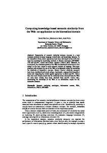
An ordered labeled tree is a tree in which the nodes are labeled and the left-to-right order among siblings is significant. Trees can represent many phenomena, such as grammar parses, image descriptions and structured texts, to name a couple. In many applications where trees are useful representations of objects, the need for comparing trees frequently arises. The tree edit distance metric was introduced by Tai [9] as a generalization of the string edit distance problem [11]. Given two trees T1 and T2 , the tree edit distance between T1 and T2 is the minimum cost of transforming one tree into the other, with the sibling and ancestor orders preserved, by a sequence of edit operations on the nodes (substitution, insertion and deletion) as shown in Figure 2.1. In the same Q article, an algorithm was given with a time complexity O(|T1 |×|T2 |× 2i=1 depth2 (Ti )).

Later, Zhang and Shasha presented an algorithm [12] which improved the running Q time to O(|T1 | × |T2 | × 2i=1 min{depth(Ti ), leaves(Ti )}). Subsequent developments were made by Klein in [5] and by Demaine et al. in [3] where the ideas were similar

6

T1

T2 (a → b) a

b

(a) substitution T2

T1 (c → ∅) c

(b) deletion T1

T2 (∅ → c)

c

(c) insertion

Figure 2.1: Tree edit operations. variants to that of Zhang and Shasha. The Klein algorithm runs in O(|T1 |2 × |T2 | × |T2 | log |T2 |) time and the Demaine et al. algorithm runs in O(|T1 |2 × |T2 | × (1 + log |T )) 1|

time. These three algorithms require quadratic space. Table 2.1 summarizes these results.

(a) (b) (c) (d)

Time Complexity Q O(|T1 | × |T2 | × 2i=1 depth2 (Ti )) Q O(|T1 | × |T2 | × 2i=1 min{depth(Ti ), leaves(Ti )}) O(|T1 |2 × |T2 | × log |T2 |) 2| )) O(|T1 |2 × |T2 | × (1 + log |T |T1 |

Worst-Case n6 n4 n3 log n n3

Table 2.1: Time complexities of known algorithms. (a): Tai. (b): Zhang-Shasha. (c): Klein. (d): Demaine et al.. For arbitrary trees, the relative running times of the last three algorithms depend on the shapes of the trees, which are not necessarily in accord with the relative order in the worst case. It is fair to say that these three algorithms represent the state of

7 the art. Therefore, our focus is on these three algorithms. All these three algorithms are based on dynamic programming with various recursion strategies prescribing the way in which a dynamic program builds up the solution. In [4], the algorithmic behaviors for each of these algorithms were formalized and the term cover strategy was used to refer to these recursion strategies. Given an instance I of the tree edit distance problem, a cover refers to a way of tree decomposition which results in a set of disjoint paths. This set of disjoint paths, which we call special paths, induces a subset of all the subproblems of I such that knowing the solutions of which is sufficient to build up the solution of I. Each special path is associated with the smallest subtree in which it is contained. The dynamic program proceeds in a bottom-up order with respect to the special paths such that for any node i on a special path, the portion of the tree below i has been processed before the node i is reached. For sibling subtrees hanging off on the sides of a special path, the decision as to which one takes precedence is referred to as strategy. In the Zhang-Shasha algorithm [12], the special paths are chosen to be the leftmost paths. In Klein’s algorithm [5] as well as that of Demaine et al. [3], the special paths are chosen such that every node on a special path is the root of a largest subtree over its sibling subtrees. These special paths are referred to as heavy paths [8]. Examples of various types of special paths are shown in Figure 2.2.

(a) leftmost paths

(b) heavy paths

(c) rightmost paths

Figure 2.2: Various types of special paths (in bold). In these algorithms, no consideration is given to any structural features which

8 may have an impact on the running time. In this paper, we investigate the possibility of utilizing certain linear features within the trees to speed up the computation. In particular, we consider two types of linearity, namely vertical linearity and horizontal linearity. We develop techniques to incorporate these types of linearity into the strategy-based algorithms. We show that the algorithmic running times of all the strategy-based algorithms may be substantially reduced in this way when there is a high degree of linearity in the input trees.

2.2 2.2.1

Preliminaries Notations

Given a tree T , we denote by t[i] the ith node in the left-to-right post-order numbering. The index of the leftmost leaf of the subtree rooted at t[i] is denoted by l(i). We denote by F [i · · · j] the ordered sub-forest of T induced by the nodes indexed i to j inclusive. The subtree rooted at t[i] in T is denoted by T [i], i.e., T [i] = F [l(i) · · · i]. The subforest induced by removing t[i] from T [i] is denoted by F [i], i.e., F [i] = F [l(i) · · · i−1]. When referring to the children of a specific node, we adopt a subscript notation in accordance with the left-to-right sibling order. For example, the children of t[i], from left to right, may be denoted by (t[i1 ], t[i2 ], · · · , t[ik ]). Denote by F • G the forest composed of forests F and G.

2.2.2

Recursion Strategy

The tree edit distance between two trees rooted respectively at the ith and the j th nodes is recursively computed according to Equation 2.1.   d(F1 [i], T2 [j]) + δ(t1 [i], ∅),    d(T1 [i], T2 [j]) = min d(T1 [i], F2 [j]) + δ(∅, t2 [j]),     d(F1 [i], F2 [j]) + δ(t1 [i], t2 [j])

        

.

(2.1)

9 In order to compute this value, we need values of some tree-to-tree distances and forest-to-forest distances that are subproblems of the given instance of problem. The tree-to-tree subproblems are computed in the same recursive fashion as in Equation 2.1. As to the forest-to-forest distance, it is recursively computed according to Equation 2.5 with base cases given in Equation 2.2, 2.3 and 2.4.

d(∅, ∅) = 0 .

(2.2)

d(F, ∅) = d(F − t[i], ∅) + δ(t[i], ∅) .

(2.3)

d(∅, G) = d(∅, G − t[j]) + δ(∅, t[j]) .

(2.4)

  d(F − t[i], G) + δ(t[i], ∅),    d(F, G) = min d(F, G − t[j]) + δ(∅, t[j]),     d(F − T [i], G − T [j]) + d(T [i], T [j])

        

.

(2.5)

There are two distinctive ways by which the forest-to-forest distance may recurse, namely the rightmost recursion where both t[i] and t[j] are the rightmost tree roots and the leftmost recursion where both t[i] and t[j] are the leftmost tree roots. Figure 2.3 and Figure 2.4 depict the rightmost recursion and the leftmost recursion, respectively. The subproblems with respect to the forest-to-forest distance d(F, G), excluding the trivial ones associated with single-node insertion or deletion cost as denoted by the δ terms, are represented by the following terms: d(F − t[i], G), d(F, G − t[j]), d(F − T [i], G − T [j]) and d(T [i], T [j]). Note that the set of sub-forests which are relevant to the computation of the tree edit distance is a subset of all possible sub-forests. We call this kind of sub-forest a relevant sub-forest, defined as follows.

10

1111 0000 0000 1111 0000 1111 0000 1111 0000 1111 0000 1111

11111111 0000 0000 0000 1111 0000 1111 0000 1111 0000 00001111 1111 0000 1111

0000 0000 ...1111 00001111 1111 0000 1111

1111 0000 0000 1111 ... 0000 1111 0000 1111 0000 1111 0000 1111

111 000 000 111 000 111 000 111 000 111 000 111

111 000 000 111 000 111 000 111 000 111 000 111

111 000 000 111 000 111 000 111 000 111 000 111

111 000 000 111 000 111 000 111 000 111 000 111

(a) deletion 1111 0000 0000 1111 0000 1111 0000 1111 0000 1111 0000 1111

11111111 0000 0000 0000 1111 0000 1111 0000 1111 0000 00001111 1111 0000 1111

0000 0000 ...1111 00001111 1111 0000 1111

1111 0000 0000 1111 ... 0000 1111 0000 1111 0000 1111 0000 1111

(b) insertion

1111 0000 0000 1111 0000 1111 0000 1111 0000 1111 0000 1111

11111111 0000 0000 0000 1111 0000 1111 0000 1111 0000 00001111 1111 0000 1111

0000 0000 ...1111 00001111 1111 0000 1111

1111 0000 0000 1111 0000 1111 0000 1111 0000 0000 1111 ... 1111 0000 1111 0000 1111 0000 1111 0000 1111 0000 1111 0000 1111 0000 1111 0000 1111 0000 0000 1111 1111 00001111 0000 1111

(c) match

Figure 2.3: Rightmost recursion.

1111 0000 0000 1111 0000 1111 0000 1111 0000 1111 0000 1111 0000 1111

1111 0000 000 111 0000 1111 000 111 0000 1111 000 ... 111 0000 1111 111 000 0000 1111 000 111 0000 1111 000 111 0000 1111 000 111

1111 0000 0000 1111 0000 1111 0000 1111 0000 1111 0000 1111 0000 1111

1111 0000 0000 1111 0000 1111 0000 1111 0000 1111 0000 ...1111 0000 1111 0000 1111 0000 1111 0000 1111 0000 1111 0000 0000 1111 1111 0000 1111

(a) deletion 111 000 000 111 000 111 000 111 000 111 000 111 000 111

111 000 000 111 000 111 000 111 000 111 000 111 000 111

1111 0000 0000 1111 0000 1111 0000 1111 0000 1111

0000 ...1111 0000 1111

111 000 000 111 000 111 000 111 000 111 000 111 000 111

111 000 000 111 000 111 ... 000 111 000 111 000 111 000 111

111 000 000 111 000 111 000 111 000 111 000 111 000 111

(b) insertion 111 000 000 111 000 111 000 111 000 111 000 111 000 111

1111 0000 000 111 0000 1111 000 111 0000 1111 000 ... 111 0000 1111 111 000 0000 1111 000 111 0000 1111 000 111 0000 1111 000 111

1111 0000 0000 1111 0000 1111 0000 1111 0000 1111 0000 1111 0000 1111

111 000 0000 1111 000 111 0000 1111 000 111 0000 ...1111 000 111 0000 1111 000 111 0000 1111 000 111 0000 000 1111 111 0000 1111

(c) match

Figure 2.4: Leftmost recursion.

11 Definition 2.1 (Relevant Sub-forest). A sub-forest appearing in a subproblem is a relevant sub-forest. Analogously, a relevant subtree is a special case of relevant sub-forest. Therefore in the preceding context, the terms F − t[i], F − T [i] and T [i] represent the relevant sub-forests with respect to F . The Zhang-Shasha algorithm is based on the rightmost recursion. Figure 2.5 gives an example showing the relevant sub-forests resulted from successive deletion of nodes in the Zhang-Shasha algorithm. In the context of dynamic programming, one would simply reverse the directions of the arrows in the example to obtain the bottomup orderings. Figure 2.6 gives an example of the entire set of relevant sub-forests generated by the recursion in the Zhang-Shasha algorithm.

11 3

3

10

7 6

1

8

9

1

6

2

5

8 4

9

1 4

3

3

1

8

3

7

1

2

7 6

1 4

5

5

9

5

6

2 4

5

2 4

6 2

1

5

3

3

1

7

6

2 4

3

10

7

2

8 4

5

3

2

1

2

1

2

1

4

Figure 2.5: An example showing the relevant sub-forests resulted from successive deletion of nodes in the Zhang-Shasha algorithm. The black nodes belong to the special path. The idea of the Klein algorithm is a similar variant of the Zhang-Shasha algorithm. The main difference is in the choice of key roots which yields special paths that may lie in the middle of a subtree. Suppose that the dynamic program encounters two forests ({T1 [ik′ ], · · · , T1 [ik ]} , {T2 [jl′ ], · · · , T2 [jl ]}) during the computation and the

12

3

11 8

3

6 1 10

2

8 4

9

3

10

7 6

2

8

3

9

1

2

8

5

4

3

2

1 4

5

1

2

1

2 3

7

5

2

3 6

6 4

9

5

7 6

1

5

5

7

4

8 4

6 1

2

9

9 8

3

7

8

10

7 6

1

9

1

2

4

1

2

4

5 3

6

5 4

4

5

1

5

2

4

5

4

Figure 2.6: An example showing the entire set of relevant sub-forests generated in the Zhang-Shasha algorithm. The black nodes belong to a special path.

13 heavy paths are identified for T1 . Let t1 [ip ], ik′ ≤ ip ≤ ik , be a special child. The Klein algorithm works as follows. If ip = ik′ , the algorithm applies rightmost recursion. If ip 6= ik′ , the algorithm applies leftmost recursion. Figure 2.7 gives an example showing the relevant sub-forests resulted from successive deletion of nodes in the Klein algorithm. Figure 2.8 gives an example of the entire set of relevant sub-forests generated by the recursion in the Klein algorithm.

11 3

3

2

8 4

2 4

9

1

2

5

8 4

9

5

5

7

10

7

6 9

6 8

5

4

7

10

7

6 8

4

6 8

9

10

7

6 1

6 1

10

7

10

7

9

2

5

8 4

9

5

7

6

6

6

8 4

5

4

5

4

5

4

5

5

Figure 2.7: An example showing the relevant sub-forests resulted from successive deletion of nodes in the Klein algorithm. The black nodes belong to the special path. In order to guarantee that the solutions to all the subproblems are available when needed during the course of the dynamic program, for each relevant sub-forest of T1 we need to consider all possible sub-forests in T2 . Demaine et al. gave a new algorithm based on a subtle modification of the Klein algorithm. Note that the Klein algorithm identifies all the special paths of the larger tree which give rise to the relevant subtrees in the larger tree. The relevant subtrees, together with all the possible sub-forests of the smaller tree form the set of subproblems. For every subproblem, the subtree of the initially larger tree guides the recursion of the dynamic program. The modification made by Demaine et al. is that, for a subproblem d(T1 [i], T2 [j]) with |T1 [i]| ≥ |T2 [j]|, instead of identifying all

14

11 3

10

7

6 1

2

8

6 1

2

8 4

10

7

4

9

9

5

5 3 1

3

2

6 2

8 4

2

7

9

5 4

9

5

8 4

9

5

10

6 8

7

9

8

5

9

9

8

6 8 4

6

8

9

4

4

5

5

7 6 4

6 2

10

7

10

7

6 8

4

2

10

7

1

1 1

4

5

5

5

Figure 2.8: An example showing the entire set of relevant sub-forests generated in the Klein algorithm. The black nodes belong to a special path.

15 the special paths of T1 [i] only the longest special path of T1 [i] is identified which gives rise to the top-level relevant subtrees of T1 [i]. On the T2 [j] side, we consider all possible sub-forests. This produces a set of smaller subproblems. The same procedure is performed recursively for each subproblem in this set. For each subproblem, the larger subtree guides the recursion of the dynamic program.

2.3

Linearity

We formally define what we mean by linearity. Based on this definition, we construct compact representation for trees. The use of such compact representation can aid in improving the running time for computing the tree edit distance. Definition 2.2 (V-Component). Given a tree T , a path π of T is a v-component (i.e., vertically linear component) if π is a maximal non-branching path. Definition 2.3 (V-Reduction). The v-reduction on a tree is to replace every vcomponent in the tree by a single node. Definition 2.4 (H-Component). Given a tree T and another tree Te obtained by a

v-reduction on T , any set of connected subgraphs of T corresponding to a set of leaves e in Te form an h-component (i.e., horizontally linear component) if L e is a maximal L e ≥ 2. contiguous subset of siblings such that |L|

Definition 2.5 (H-Reduction). The h-reduction on a tree is to replace every hcomponent in the tree by a single node. A tree possesses vertical (horizontal) linearity if it contains any v-component (hcomponent). A tree is v-reduced if it is obtained by a v-reduction only. A tree is vh-reduced if it is obtained by a v-reduction followed by an h-reduction. In Figure 2.9, we give an example showing the v-components and h-components of a tree and the corresponding reduced trees. Note that an h-component can also contain v-components.

16

v−reduced

h−reduced

Figure 2.9: An example of reduced trees as a result of compaction of nodes. The parts of the original tree affected by the compaction are represented by black nodes in the reduced tree. The v-components are shown within dashed enclosures and the h-components are shown within dotted enclosures. Each node in a v-reduced tree corresponds to either a v-component or a single node in the corresponding full tree. Given a v-reduced tree Te, we define two functions α(i) and β(i) which respectively map a node e t[i] to the highest indexed node t[α(i)]

and the lowest indexed node t[β(i)] of the corresponding v-component in the full tree T . In the special case when e t[i] corresponds to a single node in T , t[α(i)] = t[β(i)].

An example of this mapping is given in Figure 2.10. When Te is h-reduced to yield Tb, α(i) and β(i) apply in the same way to the mapping between Tb and Te.

It is important to note that a reduced tree is just a compact representation of

the original tree. Therefore, given trees (T1 , T2 ) and their reduced trees (Te1 , Te2 ), the

relation d(Te1 , Te2 ) = d(T1 , T2 ) is implied.

2.4

Incorporating Vertical Linearity

The Zhang-Shasha algorithm is conceptually the simplest to understand. Therefore we choose this algorithm to demonstrate the techniques of incorporating vertical linearity. We will then show that the techniques can apply to the entire family of

17

t[α(i)] e t[i] t[β(i)]

..... ..... T [α(i)]

Te[i]

Figure 2.10: A partial view of the mapping of nodes between a tree (left) and its v-reduced tree (right). cover strategy-based algorithms.

2.4.1

The Zhang-Shasha Algorithm

The Zhang-Shasha algorithm is based on the following recursions. Lemma 2.1. [12] 1. d(∅, ∅) = 0. 2. ∀i ∈ T1 , ∀i′ ∈ {l(i), · · · , i}, d(F1 [l(i) · · · i′ ], ∅) = d(F1 [l(i) · · · i′ − 1], ∅) + d(t1 [i′ ], ∅) .

3. ∀j ∈ T2 , ∀j ′ ∈ {l(j), · · · , j}, d(∅, F2 [l(j) · · · j ′ ]) = d(∅, F2 [l(j) · · · j ′ − 1]) + d(∅, t2 [j ′ ]) .

Lemma 2.2. [12] ∀(i, j) ∈ (T1 , T2 ), ∀i′ ∈ {l(i), · · · , i} and ∀j ′ ∈ {l(j), · · · , j},

18 if l(i′ ) = l(i) and l(j ′ ) = l(j), d(F1 [l(i) · · · i′ ], F2 [l(j) · · · j ′ ]) =   d(F1 [l(i) · · · i′ − 1], F2 [l(j) · · · j ′ ]) + d(t1 [i′ ], ∅),    min d(F1 [l(i) · · · i′ ], F2 [l(j) · · · j ′ − 1]) + d(∅, t2 [j ′ ]),     d(F1 [l(i) · · · i′ − 1], F2 [l(j) · · · j ′ − 1]) + d(t1 [i′ ], t2 [j ′ ])

     ;    

otherwise, d(F1 [l(i) · · · i′ ], F2 [l(j) · · · j ′ ]) =   d(F1 [l(i) · · · i′ − 1], F2 [l(j) · · · j ′ ]) + d(t1 [i′ ], ∅),    min d(F1 [l(i) · · · i′ ], F2 [l(j) · · · j ′ − 1]) + d(∅, t2 [j ′ ]),     d(F1 [l(i) · · · l(i′ ) − 1], F2 [l(j) · · · l(j ′ ) − 1]) + d(T1 [i′ ], T2 [j ′ ])

     .    

The main loop body of the Zhang-Shasha algorithm is shown in Algorithm 1. Each loop computes a subtree-subtree distance where the roots of the subtrees are referred to as LR-keyroots. Algorithm 1: Computing d(T1 , T2 ) input : (T1 , T2 ) output: d(T1 [i], T2 [j]), where 1 ≤ i ≤ |T1 | and 1 ≤ j ≤ |T2 | 1 2 3 4 5 6 7 8 9

compute keyroots(T1 ) and keyroots(T2 ) sort (keyroots(T1 ), keyroots(T2 )) in increasing order into arrays (K1 , K2 ) for i′ ← 1 to |keyroots(T1 )| do for j ′ ← 1 to |keyroots(T2 )| do i ← K1 [i′ ] j ← K2 [j ′ ] LRKeyRoots(i, j) endfor endfor

19

Algorithm 2: LRKeyRoots(i, j) 1 d(∅, ∅) ← 0 ′ 2 for i ← l(i) to i do 3 d(F1 [l(i) · · · i′ ], ∅) ← d(F1 [l(i) · · · i′ − 1], ∅) + d(t1 [i′ ], ∅) 4 endfor ′ 5 for j ← l(j) to j do 6 d(∅, F2 [l(j) · · · j ′ ]) ← d(∅, F2 [l(j) · · · j ′ − 1]) + d(∅, t2 [j ′ ]) 7 endfor ′ 8 for i ← l(i) to i do 9 for j ′ ← l(j) to j do 10 if l(i′ ) = l(i) and l(j ′ ) = l(j) then 11 d(F1 [l(i) · · · i′ ], F2 [l(j) · · · j ′ ]) ← d(F1 [l(i) · · · i′ − 1], F2 [l(j) · · · j ′ ]) + d(t1 [i′ ], ∅),    d(F1 [l(i) · · · i′ ], F2 [l(j) · · · j ′ − 1]) + d(∅, t2 [j ′ ]), min d(F1 [l(i) · · · i′ − 1], F2 [l(j) · · · j ′ − 1])    +d(t1 [i′ ], t2 [j ′ ]) 12 d(T1 [i′ ], T2 [j ′ ]) ← d(F1 [l(i) · · · i′ ], F2 [l(j) · · · j ′ ]) 13 endif 14 else 15 d(F1 [l(i) · · · i′ ], F2 [l(j) · · · j ′ ]) ← d(F1 [l(i) · · · i′ − 1], F2 [l(j) · · · j ′ ]) + d(t1 [i′ ], ∅),    d(F1 [l(i) · · · i′ ], F2 [l(j) · · · j ′ − 1]) + d(∅, t2 [j ′ ]), min d(F1 [l(i) · · · l(i′ ) − 1], F2 [l(j) · · · l(j ′ ) − 1])    +d(T1 [i′ ], T2 [j ′ ]) 16 endif 17 endfor 18 endfor

      

      

20

2.4.2

Properties

We denote by d(x, y) the edit distance between x and y. The following lemmas incorporate vertical linearity in the Zhang-Shasha algorithm. Lemma 2.3. 1. d(∅, ∅) = 0. 2. ∀i ∈ Te1 , ∀i′ ∈ {l(i), · · · , i}, d(Fe1 [l(i) · · · i′ ], ∅) = d(Fe1 [l(i) · · · i′ − 1], ∅) + d(e t1 [i′ ], ∅) . 3. ∀j ∈ Te2 , ∀j ′ ∈ {l(j), · · · , j}, d(∅, Fe2 [l(j) · · · j ′ ]) = d(∅, Fe2 [l(j) · · · j ′ − 1]) + d(∅, e t2 [j ′ ]) . Proof. Case 1 requires no edit operation. In case 2 and case 3, the distances correspond to the costs of deleting and inserting the nodes in Fe1 [l(i) · · · i′ ] and Fe2 [l(j) · · · j ′ ],

respectively.

Lemma 2.4. ∀(i, j) ∈ (Te1 , Te2 ), ∀i′ ∈ {l(i), · · · , i} and ∀j ′ ∈ {l(j), · · · , j},

if l(i′ ) = l(i) and l(j ′ ) = l(j),

d(Fe1 [l(i) · · · i′ ], Fe2 [l(j) · · · j ′ ]) = d(Te1 [i′ ], Te2 [j ′ ]) ; otherwise, d(Fe1 [l(i) · · · i′ ], Fe2 [l(j) · · · j ′ ]) =   d(Fe1 [l(i) · · · i′ − 1], Fe2 [l(j) · · · j ′ ]) + d(e t1 [i′ ], ∅),    min d(Fe1 [l(i) · · · i′ ], Fe2 [l(j) · · · j ′ − 1]) + d(∅, e t2 [j ′ ]),     e d(F1 [l(i) · · · l(i′ ) − 1], Fe2 [l(j) · · · l(j ′ ) − 1]) + d(Te1 [i′ ], Te2 [j ′ ])

        

.

21 Proof. The condition “l(i′ ) = l(i) and l(j ′ ) = l(j)” implies that the two forests are simply two trees and the equality clearly holds. We now consider the other condition in which “l(i′ ) 6= l(i) or l(j ′ ) 6= l(j)”. If t1 [α(i′ )] = t1 [β(i′ )] and t2 [α(j ′ )] = t2 [β(j ′ )], the formula holds as an obvious result. Otherwise, at least one of e t1 [i′ ] and e t2 [j ′ ] corresponds to a v-component in (T1 [α(i)], T2 [α(j)]). Consider the components in

(T1 [α(i)], T2 [α(j)]) corresponding to (e t1 [i′ ], e t2 [j ′ ]). There are two cases to consider:

either (1) there is no occurrence of node-to-node match between the components; or

(2) there is at least one occurrence of node-to-node match between the components. In case 1, one of the components must be entirely deleted which implies that either e t1 [i′ ] must be deleted or e t2 [j ′ ] must be inserted. In case 2, in order to preserve the ancestor-descendant relationship Te1 [i′ ] and Te2 [j ′ ] must be matched.

Note. In Lemma 2.4 for the condition “l(i′ ) 6= l(i) or l(j ′ ) 6= l(j)” the value of d(Te1 [i′ ], Te2 [j ′ ]) would already be available if implemented in a bottom-up order, since it

involves a subproblem of d(Fe1 [l(i) · · · i′ ], Fe2 [l(j) · · · j ′ ]) and would have been computed. For the condition “l(i′ ) = l(i) and l(j ′ ) = l(j)”, however, we encounter the problem involving (Te1 [i′ ], Te2 [j ′ ]) for the first time and must compute its value. We show how to compute d(Te1 [i′ ], Te2 [j ′ ]) in the following lemmas.

Lemma 2.5. ∀u ∈ {β(i′ ), · · · , α(i′ )},

d(T1 [u], F2 [β(j ′ )]) =    d(F1 [u], F2 [β(j ′ )]) + d(t1 [u], ∅),  . min  min ′  ′ j1 ≤q≤jl′ {d(T1 [u], T2 [α(q)]) − d(∅, T2 [α(q)])} + d(∅, F2 [β(j )]) Proof. This is the edit distance between the tree T1 [u] and the forest F2 [β(j ′ )]. There are two cases. In the first case, t1 [u] is constrained to be deleted and the remaining substructure F1 [u] is matched to F2 [β(j ′ )]. In the second case, t1 [u] is constrained to be matched to a node somewhere in F2 [β(j ′ )]. This is equivalent to stating that T1 [u] is constrained to be matched to a subtree in F2 [β(j ′ )]. The question thus becomes

22 finding a subtree in F2 [β(j ′ )] to be matched to T1 [u] so as to minimize the distance between T1 [u] and F2 [β(j ′ )] under such constraint. This can be done by considering the set of all combinations in which exactly one tree in F2 [β(j ′ )] is matched to T1 [u] while the remainder of F2 [β(j ′ )] is deleted. The minimum in this set is the edit distance for the second case. Lemma 2.6. ∀v ∈ {β(j ′ ), · · · , α(j ′ )}, d(F1 [β(i′ )], T2 [v]) =    d(F1 [β(i′ )], F2 [v]) + d(∅, t2 [v]),  . min  min ′  ′ i1 ≤p≤i′k {d(T1 [α(p)], T2 [v]) − d(T1 [α(p)], ∅)} + d(F1 [β(i )], ∅) Proof. This is symmetric to that of Lemma 2.5. Lemma 2.7. ∀u ∈ {β(i′ ), · · · , α(i′ )} and ∀v ∈ {β(j ′ ), · · · , α(j ′ )},   d(F1 [u], T2 [v]) + d(t1 [u], ∅),    d(T1 [u], T2 [v]) = min d(T1 [u], F2 [v]) + d(∅, t2 [v]),     d(F1 [u], F2 [v]) + d(t1 [u], t2 [v])

        

.

Proof. This is a known result for the tree-to-tree edit distance. Note. In the computation for every d(Te1 [i′ ], Te2 [j ′ ]), we save the values of d(T1 [u], T2 [α(j ′ )]) for all u ∈ {β(i′ ), · · · , α(i′ )} and d(T1 [α(i′ )], T2 [v]) for all v ∈

{β(j ′ ), · · · , α(j ′ )}. This ensures that when d(T1 [u], F2 [β(j ′ )]) in Lemma 2.5 and d(F1 [β(i′ )], T2 [v]) in Lemma 2.6 are evaluated in a bottom-up order the values of the terms involving d(T1 [u], T2 [α(q)]) and d(T1 [α(p)], T2 [v]) would be available. Lemma 2.8. d(Te1 [i′ ], Te2 [j ′ ]) = d(T1 [α(i′ )], T2 [α(j ′ )]) .

Proof. The result follows from the tree definitions.

We give figures to illustrate the above lemmas for computing d(Te1 [i′ ], Te2 [j ′ ]) as

follows. When this subproblem comes into scene for the first time during the compu-

23 tation, d(F1 [β(i′ )], F2 [β(j ′ )]) has already been computed. This situation is depicted in Figure 2.11. The computation proceeds by executing the lemmas in the following order: Lemma 2.5, Lemma 2.6, Lemma 2.7. The scenarios for these lemmas are depicted in Figure 2.12, 2.13 and 2.14.

11 00 00 11 00 11 00 11 00 11

... (a)

11 00 00 11 00 11 00 11 00 11

111 000 000 111 000 111 000 111 000 111

000 111 111 ... 000 000 111 000 111 (b)

000 111

Figure 2.11: F1 [β(i′ )] and F2 [β(j ′ )].

11 00 00 11 00 11 00 11

... (a)

11 00 00 11 00 11 00 11

111 000 000 111 000 111 000 111

000 ... 111 000 111 000 111 (b)

000 111

Figure 2.12: T1 [α(i′ )] and F2 [β(j ′ )] in Lemma 2.5.

2.4.3

Algorithmic Improvements

With dynamic programming, it is possible that the solution of one subproblem may be obtained as a by-product of computing another subproblem. For example, in the rightmost recursion strategy the solutions of two subproblems may be obtained in one run of computation if the relevant sub-forests in the smaller subproblem are the prefixes of the relevant sub-forests in the larger subproblem. In this case, the solution of the smaller subproblem is obtained as a by-product of the computation of the

24

11 00 00 11 00 11 00 11

... (a)

11 00 00 11 00 11 00 11

111 000 000 111 000 111 000 111

000 ... 111 000 111 (b)

111 000 000 111

Figure 2.13: F1 [β(i′ )] and T2 [α(j ′ )] in Lemma 2.6.

11 00 00 11 00 11 00 11

... (a)

11 00 00 11 00 11 00 11

111 000 000 111 000 111 000 111

000 ... 111 000 111 000 111 (b)

000 111

Figure 2.14: T1 [α(i′ )] and T2 [α(j ′ )] in Lemma 2.7. larger subproblem. If, however, the solution of a subproblem can not be obtained as a by-product of solving another subproblem, then it must be computed separately. We refer to this kind of subproblems as disjoint subproblems. Definition 2.6 (Disjoint Subproblems). The set of disjoint subproblems is such that the solution of any member of this set can not be obtained as a by-product of solving another subproblem. For the sake of efficiency, it is crucial to identify the set of disjoint subproblems as such set forms a cover of all the subproblems the solutions of which are necessary for building the final solution. We describe an important concept, namely key roots, for the purpose of identifying the set of disjoint subproblems, as follows. For every node i of tree T , we designate a child of i, if any, to be its special child, denoted by sc(i). Note that in the Zhang-Shasha algorithm sc(i) is the leftmost child of i whereas in a different recursion strategy the choice of sc(i) may be different.

25 Denote by p(i) the parent of i. We define a set of nodes, called key roots, for tree T as follows.

keyroots(T ) = {k | k = root(T ) or k 6= sc(p(k))} . This is a generalized version of the LR keyroots used in [12] and is suitable for any known recursion strategy as in [3, 5, 12]. Referring to Figure 2.2, in every special path the highest numbered node in a left-to-right post-order is a key root. Here is the intuitive meaning of key root. Suppose, for example, that the recursion strategy is rightmost and let i ∈ keyroots(T1 ) and j ∈ keyroots(T2 ), then d(T1 [i], T2 [j]) is a disjoint subproblem; that is, it requires a separate computation. We now present the new algorithm. The entry point is Algorithm 3. Algorithm 3 contains the main loop which repeatedly calls the procedure KeyRoots to compute d(Te1 [i], Te2 [j]) where (i, j) are key roots in (Te1 , Te2 ). The procedure KeyRoots is divided

into several parts with each part handled in a separate procedure. The following notations are used. • Dt : a (|T1 | + 1) × (|T2 | + 1) two-dimensional permanent array. e t : a (|Te1 | + 1) × (|Te2 | + 1) two-dimensional permanent array. • D

e f : a (|Te1 | + 1) × (|Te2 | + 1) two-dimensional temporary array. • D

• A1 , A2 : temporary one-dimensional arrays of lengths (|T1 | + 1) and (|T2 | + 1), respectively. e t is Dt is used to store distances with respect to the (T1 , T2 ) representation. D

used to store distances with respect to the (Te1 , Te2 ) representation. The computation e f . A1 and A2 are used in conjunction with for forest-to-forest distances is done in D

e f , A1 and A2 allow Dt to handle boundary initializations. The temporary arrays D

rewriting of their contents.

Lemma 2.9. The new algorithm correctly computes d(T1 , T2 ).

26 Algorithm 3: Computing d(T1 , T2 ) input : (T1 , T2 ) e t containing d(T1 [α(i)], T2 [α(j)]), where 1 ≤ i ≤ |Te1 |, output: matrix D 1 ≤ j ≤ |Te2 | e1 , Te2 ) 1 build (T e1 ) and keyroots(Te2 ) 2 compute keyroots(T e1 ), keyroots(Te2 )) in increasing order into arrays (K1 , K2 ) 3 sort (keyroots(T ′ e1 )| do 4 for i ← 1 to |keyroots(T 5 for j ′ ← 1 to |keyroots(Te2 )| do 6 i ← K1 [i′ ] 7 j ← K2 [j ′ ] 8 KeyRoots(i, j) 9 endfor 10 endfor

Algorithm 4: KeyRoots(i, j) 1 BoundaryConditions(i, j) 2 MainRecursion(i, j)

Algorithm 5: BoundaryConditions(i, j) e f [l(i) − 1, l(j) − 1] ← 0 1 D ′ 2 for i ← l(i) to i do e f [i′ , l(j) − 1] ← D e f [i′ − 1, l(j) − 1] + δ(e 3 D t1 [i′ ], ∅) 4 endfor ′ 5 for j ← l(j) to j do e f [l(i) − 1, j ′ ] ← D e f [l(i) − 1, j ′ − 1] + δ(∅, e 6 D t2 [j ′ ]) 7 endfor Algorithm 6: MainRecursion(i, j) ′ 1 for i ← l(i) to i do 2 for j ′ ← l(j) to j do 3 if l(i′ ) = l(i) and l(j ′ ) = l(j) then 4 TreeDist(i′ , j ′ ) 5 else 6 ForestDist(i′ , j ′ ) 7 endif 8 endfor 9 endfor

27

Algorithm 7: TreeDist(i′ , j ′ ) ′ ′ 1 for u ← β(i ) − 1 to α(i ) do ′ 2 A1 [u] ← Dt [u, β(j ) − 1] 3 endfor ′ ′ 4 for v ← β(j ) to α(j ) do 5 A2 [v] ← Dt [β(i′ ) − 1, v] 6 endfor ′ ′ e f [i′ − 1, j ′ − 1] 7 Dt [β(i ) − 1, β(j ) − 1] ← D ′ ′ 8 for u ← β(i ) to α(i ) do ′ 9 Dt [u, β(j ) − 1] ←   Dt [u − 1, β(j ′ ) − 1] + δ(t1 [u], ∅), min minj1′ ≤q≤jl′ {Dt [u, α(q)] − δ(∅, T2 [α(q)])} + δ(∅, F2 [β(j ′ )]) 10 endfor ′ ′ 11 for v ← β(j ) to α(j ) do 12 Dt [β(i′ ) − 1, v] ←   Dt [β(i′ ) − 1, v − 1] + δ(∅, t2 [v]), min mini′1 ≤p≤i′k {Dt [α(p), v] − δ(T1 [α(p)], ∅)} + δ(F1 [β(i′ )], ∅) 13 endfor ′ ′ 14 for u ← β(i ) to α(i ) do ′ ′ 15 for v ← β(j ) to α(j  ) do    Dt [u − 1, v] + δ(t1 [u], ∅), Dt [u, v] ← min Dt [u, v − 1] + δ(∅, t2 [v]),   Dt [u − 1, v − 1] + δ(t1 [u], t2 [v]) 16 17 endfor 18 endfor e t [i′ , j ′ ] ← Dt [α(i′ ), α(j ′ )] 19 D e f [i′ , j ′ ] ← Dt [α(i′ ), α(j ′ )] 20 D ′ ′ 21 for u ← β(i ) − 1 to α(i ) do 22 Dt [u, β(j ′ ) − 1] ← A1 [u] 23 endfor ′ ′ 24 for v ← β(j ) to α(j ) do 25 Dt [β(i′ ) − 1, v] ← A2 [v] 26 endfor

Algorithm 8: ForestDist(i′ , j ′ )  e f [i′ − 1, j ′ ] + δ(e  t1 [i′ ], ∅),  D e f [i′ , j ′ ] ← min D e f [i′ , j ′ − 1] + δ(∅, e D t2 [j ′ ]),   D e f [l(i′ ) − 1, l(j ′ ) − 1] + D e t [i′ , j ′ ] 1

    

28 Proof. The correctness of all the computed values in the new algorithm follows from the lemmas. By Lemma 2.8, d(Te1 , Te2 ) = d(T1 , T2 ) when (i′ , j ′ ) are set to be the

roots of (Te1 , Te2 ). Since these roots are key roots, d(T1 , T2 ) is always computed by the

algorithm.

Lemma 2.10. Given T1 and T2 , the new algorithm runs in O(|T1 | × |T2 | + |Te1 | ×

|Te2 | × min{depth(Te1 ), leaves(Te1 )} × min{depth(Te2 ), leaves(Te2 )}) time and O(|T1 | ×

|T2 |) space, with |Te1 | ≤ |T1 | and |Te2 | ≤ |T2 |.

Proof. We first consider the time complexity.

Te1 and Te2 can be built in linear

time in a preprocess. Identifying and sorting the key roots can be done in linear time. All the values associated with insertion or deletion of a subtree or a sub-forest, as in Lemma 2.5 and Lemma 2.6, can be obtained beforehand in linear time during a tree traversal. The Zhang-Shasha algorithm runs in O(|Te1 | × |Te2 | × min{depth(Te1 ), leaves(Te1 )} × min{depth(Te2 ), leaves(Te2 )}) time for (Te1 , Te2 ). We con-

sider the loops in the procedure TreeDist which involve computations related to the (i′ , j ′ ) pairs on leftmost paths, based on Lemma 2.5, 2.6 and 2.7. This is the part of the algorithm that explicitly traverses in (T1 , T2 ). For each such (i′ , j ′ ) pair, this part takes O((α(i′ ) − β(i′ ) + 1) × (jl′ − j1′ + 1) + (α(j ′ ) − β(j ′ ) + 1) × (i′k − i′1 + 1) + (α(i′ ) − β(i′ ) + 1) × (α(j ′ ) − β(j ′ ) + 1)). All the subproblems associated with these (i′ , j ′ ) pairs are disjoint. Summing over all these pairs, we can bound the complexity by O(|T1 | × |T2 |). Hence, the overall time complexity follows. By considering the sizes of the data structures used, the space complexity clearly follows.

Theorem 2.1. Given (T1 , T2 ), the edit distance d(T1 , T2 ) can be computed in O(|T1 |× |T2 | + T (A, Te1 , Te2 )) time where T (A, Te1 , Te2 ) is the time complexity of any strategybased algorithm A applied to (Te1 , Te2 ).

Proof. Since a v-component corresponds to a simple path, there is only one way a dynamic program may recurse along this path regardless which strategy is used.

29 Hence, Lemma 2.5 to 2.8 are valid for all cover strategies. Lemma 2.3 and 2.4, after a proper adjustment of the subtree orderings in each forest to adapt to the given strategy, are also valid. The theorem is implied from Lemma 2.9 and 2.10 when the relevant lemmas are properly embedded in any strategy-based algorithm. The above result is an improvement over the original algorithms. This can be easily seen as |T1 | × |T2 | < T (A, T1 , T2 ) and T (A, Te1 , Te2 ) ≤ T (A, T1 , T2 ).

2.4.4

Application

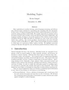
We describe one application which would benefit from our result, namely RNA secondary structure comparison. RNA is a molecule consisting of a single strand of nucleotides (abbreviated as A, C, G and U ) which folds back onto itself by means of hydrogen bonding between distant complementary nucleotides, giving rise to a so-called secondary structure. The secondary structure of an RNA molecule can be topologically represented by a tree. An example is depicted in Figure 2.15. In this representation, an internal node represents a pair of complementary nucleotides interacting via hydrogen bonding. When a number of such pairs are stacked up, they form a local structure called stem, which corresponds to a v-component in the tree representation. The secondary structure plays an important role in the functions of RNA [7]. Therefore, comparing the secondary structures of RNA molecules can help understand their comparative functions. One way to compare two trees is to compute the edit distance between them. As an example, we list the size reductions for a set of tRNA molecules in Table 2.2. The last column shows the size reductions in percentage. On average, we observe a size reduction by nearly one third of the original size, which roughly translates into a one-half decrease of running time for the known strategy-based algorithms.

30

AU GC CG C A

U

G

C

C

G

A U A C A U U U A A A U A C A U G C C U U G A U G C U G

UA

U A

A

UA

UA

AU

CG

UA

CG

GC

U C G U

UA

C

U

(a) RNA secondary structure

A U C U

(b) the corresponding tree representation

Figure 2.15: The secondary structure of RNA and the corresponding tree representation. The dotted lines in the secondary structure represent hydrogen bonds.

Name Athal-chr4.trna25 cb25.fpc2454.trna15 CHROMOSOME I.trna38 chr1.trna1190 Acinetobacter sp ADP1.trna45 Aquifex aeolicus.trna21 Azoarcus sp EbN1.trna58 Bacillus subtilis.trna63 Aeropyrum pernix K1.trna3 Sulfolobus tokodaii.trna25

|T | 52 52 51 51 55 55 55 52 56 53

|Te| 35 40 38 34 38 38 38 35 39 36

Reduction (%) 33% 23% 25% 33% 31% 31% 31% 33% 30% 32%

Table 2.2: Vertical reduction of tree sizes for selected tRNA molecules [10].

31

2.5

Incorporating Horizontal Linearity

The incorporation of horizontal linearity relies on certain properties pertaining to the edit distance between two forests both suffixed with a horizontal component. These properties allow us to relate the current problem to the problem of finding row minima in a totally monotone matrix. In the following, we describe the problem of finding row minima in a totally monotone matrix. We then identify and discuss the properties that enable us to establish the connection between this problem and the problem we want to solve. This connection makes it feasible to solve our problem by taking advantage of existing efficient algorithms for finding row minima in a totally monotone matrix.

2.5.1

Properties

Definition 2.7 (Monge Condition [6]). A cost function w satisfies the (convex) Monge condition if ∀ a < b and c < d,

w(a, c) + w(b, d) ≤ w(b, c) + w(a, d) .

Since w(a, c) − w(a, d) ≤ w(b, c) − w(b, d), therefore w(a, c) − w(a, d) ≥ 0 implies w(b, c) − w(b, d) ≥ 0. This leads to the following property. Definition 2.8 (Totally Monotone Matrix [1]). An m×n matrix A is (convex) totally monotone if and only if ∀ a < b and c < d,

A[a, c] ≥ A[a, d] ⇒ A[b, c] ≥ A[b, d] .

We now define some shorthand notations related to an m × n matrix A. Denote by row(A, i) and col(A, j) the ith row and the jth column of A, respectively. Denote by A[i · · · i′ , j · · · j ′ ] the sub-matrix of A that is the intersection of rows row(A, i), · · · , row(A, i′ ) and columns col(A, j), · · · , col(A, j ′ ).

32 Denote

by

indmin(row(A, i))

the

minimum

column

index

such

that

A[i, indmin(row(A, i))] equals the minimum value in row(A, i). An important consequence of totoal monotonicity is

indmin(row(A, 1)) ≤ indmin(row(A, 2)) ≤ · · · ≤ indmin(row(A, n)) .

One problem which is closely related to our purpose and can be solved efficiently by taking advantage of the total monotonicity is the problem of finding row minima for a totally monotone matrix. To find the row minima of a totally monotone matrix Am×n , a linear time solution is available [1]. The solution is given in Algorithm 10 which executes Algorithm 9 in the first step. The time complexity is O(m + n) and the space complexity is O(max{m, n}). Algorithm 9: [1]Reduce(Am×n ) 1 B ← A 2 i ← 1 3 while number of columns in B > m do 4 if B[i, i] ≥ B[i, i + 1] then 5 delete col(B, i) 6 i ← min {1, i − 1} 7 else 8 if i < m then 9 i←i+1 10 else 11 delete col(B, i + 1) 12 endif 13 endif 14 endw 15 return B

In our problem setting, we are concerned with a pair of forests of the form (F • h1 [1 · · · l1 ], G•h2 [1 · · · l2 ]) where h1 and h2 represent two sequences of nodes of lengths l1 and l2 , respectively. The dynamic programming table corresponding to this part of the computation is depicted in Figure 2.16. The lower-right block of the table corresponds to d(F •h1 [1 · · · i], G•h2 [1 · · · j]) for 1 ≤ i ≤ l1 and 1 ≤ j ≤ l2 . Recursively

33

Algorithm 10: [1]RowMin(Am×n ) 1 B ← Reduce(A) 2 if m = 1 then 3 output the minimum and return 4 endif 5 C ← {row(B, 2), row(B, 4), · · · , row(B, 2 × ⌊m/2⌋)} 6 RowMin(C) 7 from the known positions of the minima in the even rows of B, find the minima in its odd rows

G

h2

F

h1

111111 000000 000000 111111 000000 111111 000000 111111 000000 111111 000000 111111 000000 111111 000000 111111 000000 111111

Figure 2.16: Dynamic programming table for d(F • h1 , G • h2 ).

34 throughout the entire (F • h1 [1 · · · l1 ], G • h2 [1 · · · l2 ]), our objective is that instead of computing all the (l1 × l2 ) entries corresponding to d(F • h1 [1 · · · i], G • h2 [1 · · · j]) for 1 ≤ i ≤ l1 and 1 ≤ j ≤ l2 , we compute only (l1 + l2 − 1) entries corresponding to d(F • h1 [1 · · · i], G • h2 [1 · · · l2 ]) for 1 ≤ i ≤ l1 and d(F • h1 [1 · · · l1 ], G • h2 [1 · · · i]) for 1 ≤ i ≤ l2 as highlighted by the shaded region in the lower-right block. The matter of fact is that computing only these entries instead of the entire block is sufficient for the computation to continue beyond this pair of forests. However, this also incurs an additional treatment in order to carry out the computation in this fashion. The justification of this approach is that the time saved on the omitted computation exceeds the time spent in carrying out the additional treatment. We describe this approach as follows. The next two lemmas describe what information is involved in computing d(F • h1 [1 · · · i], G • h2 [1 · · · l2 ]) for 1 ≤ i ≤ l1 and d(F • h1 [1 · · · l1 ], G • h2 [1 · · · i]) for 1 ≤ i ≤ l2 . Lemma 2.11. ∀i ∈ {1, · · · , l1 }, d(F • h1 [1 · · · i], G • h2 [1 · · · l2 ]) =    min0≤j≤i {d(F • h1 [1 · · · j], G) + d(h1 [j + 1 · · · i], h2 [1 · · · l2 ])} ,  . (2.6) min  min {d(F, G • h [1 · · · j]) + d(h [1 · · · i], h [j + 1 · · · l ])}  0≤j≤l2

2

1

2

2

Proof. Denote by hF, Gi the edit script for d(F, G). We partition (F • h1 [1 · · · i], G • h2 [1 · · · l2 ]) into P1 = (F • h1 [1 · · · p], G • h2 [1 · · · q]) and P2 = (h1 [p + 1 · · · i], h2 [q + 1 · · · l2 ]) such that the leftmost edit step ha, bi in hF • h1 [1 · · · i], G • h2 [1 · · · l2 ]i where a ∈ h1 [1 · · · i] and b ∈ h2 [1 · · · l2 ], if one exists, is hh1 [p + 1], h2 [q + 1]i. If such edit step does not exist, then P2 = ∅. As to h1 [1 · · · p] and h2 [1 · · · q], since there can not exist any match between them (otherwise, hh1 [p + 1], h2 [q + 1]i would not be the leftmost edit step we are seeking), they can either involve indels only or matches with G or F . There are three cases.

35 1. h1 [1 · · · p] and h2 [1 · · · q] involve only indels: d(F • h1 [1 · · · i], G • h2 [1 · · · l2 ]) = d(F • h1 [1 · · · p], G) + d(h1 [p + 1 · · · i], h2 [1 · · · l2 ]) = d(F, G • h2 [1 · · · q]) + d(h1 [1 · · · i], h2 [q + 1 · · · l2 ]) .

2. h1 [1 · · · p] involves matches with G and h2 [1 · · · q] involves indels only: d(F • h1 [1 · · · i], G • h2 [1 · · · l2 ]) = d(F • h1 [1 · · · p], G) + d(h1 [p + 1 · · · i], h2 [1 · · · l2 ]). 3. h1 [1 · · · p] involves indels only and h2 [1 · · · q] involves matches with F : d(F • h1 [1 · · · i], G • h2 [1 · · · l2 ]) = d(F, G • h2 [1 · · · q]) + d(h1 [1 · · · i], h2 [q + 1 · · · l2 ]). Note that it is not possible that both h1 [1 · · · p] and h2 [1 · · · q] involve matches with G and F , respectively, since this would violate the basic requirement that the ordering of the tree nodes be preserved in the edit script. Putting together these cases, we have d(F • h1 [1 · · · i], G • h2 [1 · · · l2 ]) =    d(F • h1 [1 · · · p], G) + d(h1 [p + 1 · · · i], h2 [1 · · · l2 ]),  . min  d(F, G • h [1 · · · q]) + d(h [1 · · · i], h [q + 1 · · · l ])  2

1

2

2

For a fixed i, let

A = {d(F • h1 [1 · · · j], G) + d(h1 [j + 1 · · · i], h2 [1 · · · l2 ]) | 0 ≤ j ≤ i} , B = {d(F, G • h2 [1 · · · j]) + d(h1 [1 · · · i], h2 [j + 1 · · · l2 ]) | 0 ≤ j ≤ l2 } . The elements of A ∪ B are generated from all possible partitions on (F • h1 [1 · · · i], G • h2 [1 · · · l2 ]). Therefore, d(F • h1 [1 · · · i], G • h2 [1 · · · l2 ]) is the minimum element in A ∪ B.

36 Lemma 2.12. ∀i ∈ {1, · · · , l2 }, d(F • h1 [1 · · · l1 ], G • h2 [1 · · · i]) =    min0≤j≤i {d(F, G • h2 [1 · · · j]) + d(h1 [1 · · · l1 ], h2 [j + 1 · · · i])} ,  . (2.7) min  min  0≤j≤l1 {d(F • h1 [1 · · · j], G) + d(h1 [j + 1 · · · l1 ], h2 [1 · · · i])} Proof. Symmetrical to Lemma 2.11. To obtain d(F • h1 [1 · · · i], G • h2 [1 · · · l2 ]) or d(F • h1 [1 · · · l1 ], G • h2 [1 · · · i]), we need the values of the set of individual terms from which the minima are obtained. As will be shown later, the crucial task is obtaining the following terms efficiently: d(h1 [j +1 · · · i], h2 [1 · · · l2 ]), d(h1 [1 · · · i], h2 [j +1 · · · l2 ]), d(h1 [1 · · · l1 ], h2 [j +1 · · · i]) and d(h1 [j + 1 · · · l1 ], h2 [1 · · · i]). We now discuss some crucial relations among these terms that allow us to transform this part of computation to the problem of finding row minima for totally monotone matrices which can be solved by Algorithm 10. Lemma 2.13. Let Dij = d(F • h1 [1 · · · j], G) + d(h1 [j + 1 · · · i], h2 [1 · · · l2 ]). For any 0 ≤ j ≤ j ′ ≤ i ≤ i′ ≤ l1 , Dij + Di′ j ′ ≤ Dij ′ + Di′ j . Proof. Define dij = d(h1 [j + 1 · · · i], h2 [1 · · · l2 ]) , then Dij = d(F • h1 [1 · · · j], G) + dij . Since Dij + Di′ j ′ = d(F • h1 [1 · · · j], G) + d(F • h1 [1 · · · j ′ ], G) + dij + di′ j ′ , and Dij ′ + Di′ j = d(F • h1 [1 · · · j], G) + d(F • h1 [1 · · · j ′ ], G) + dij ′ + di′ j ,

37 after cancellation of terms our task reduces to proving

dij + di′ j ′ ≤ dij ′ + di′ j , that is, d(h1 [j + 1 · · · i], h2 [1 · · · l2 ]) + d(h1 [j ′ + 1 · · · i′ ], h2 [1 · · · l2 ]) ≤ d(h1 [j ′ + 1 · · · i], h2 [1 · · · l2 ]) + d(h1 [j + 1 · · · i′ ], h2 [1 · · · l2 ]) . Denote by pij a minimum-cost edit path for (h1 [j + 1 · · · i], h2 [1 · · · l2 ]) with a cost equal dij . Since h1 [j + 1 · · · i′ ] contains h1 [j ′ + 1 · · · i], pij ′ and pi′ j must meet at some point. This means that ∃(k, l) where j ′ ≤ k ≤ i and 0 ≤ l ≤ l2 , such that dij ′ = d(h1 [j ′ + 1 · · · i], h2 [1 · · · l2 ]) = d(h1 [j ′ + 1 · · · k], h2 [1 · · · l]) + d(h1 [k + 1 · · · i], h2 [l + 1 · · · l2 ]) and di′ j = d(h1 [j + 1 · · · i′ ], h2 [1 · · · l2 ]) = d(h1 [j + 1 · · · k], h2 [1 · · · l]) + d(h1 [k + 1 · · · i′ ], h2 [l + 1 · · · l2 ]) . See Figure 2.17 for an example. Therefore,

dij ′ + di′ j = d(h1 [j ′ + 1 · · · k], h2 [1 · · · l]) + d(h1 [k + 1 · · · i], h2 [l + 1 · · · l2 ]) +d(h1 [j + 1 · · · k], h2 [1 · · · l]) + d(h1 [k + 1 · · · i′ ], h2 [l + 1 · · · l2 ]) = (d(h1 [j ′ + 1 · · · k], h2 [1 · · · l]) + d(h1 [k + 1 · · · i′ ], h2 [l + 1 · · · l2 ])) +(d(h1 [j + 1 · · · k], h2 [1 · · · l]) + d(h1 [k + 1 · · · i], h2 [l + 1 · · · l2 ])) .

38 0

l

l2

0

j+1

j′ + 1 k i

i′

l1

Figure 2.17: An example for Lemma 2.13. Note that d(h1 [j ′ + 1 · · · k], h2 [1 · · · l]) + d(h1 [k + 1 · · · i′ ], h2 [l + 1 · · · l2 ]) and d(h1 [j + 1 · · · k], h2 [1 · · · l]) + d(h1 [k + 1 · · · i], h2 [l + 1 · · · l2 ]) correspond to the costs of some edit paths for (h1 [j ′ + 1 · · · i′ ], h2 [1 · · · l2 ]) and (h1 [j + 1 · · · i], h2 [1 · · · l2 ]), respectively. Since the minimum costs for (h1 [j ′ + 1 · · · i′ ], h2 [1 · · · l2 ]) and (h1 [j + 1 · · · i], h2 [1 · · · l2 ]) are di′ j ′ and dij , respectively, it follows that dij + di′ j ′ ≤ dij ′ + di′ j , hence Dij + Di′ j ′ ≤ Dij ′ + Di′ j . Lemma 2.14. Let Dij = d(F, G • h2 [1 · · · j]) + d(h1 [1 · · · i], h2 [j + 1 · · · l2 ]). For any 1 ≤ i ≤ i′ ≤ l1 and 0 ≤ j ≤ j ′ ≤ l2 , Dij + Di′ j ′ ≥ Dij ′ + Di′ j . Proof. Define dij = d(h1 [1 · · · i], h2 [j + 1 · · · l2 ]) , then Dij = d(F, G • h2 [1 · · · j]) + dij .

39 Since Dij + Di′ j ′ = d(F, G • h2 [1 · · · j]) + d(F, G • h2 [1 · · · j ′ ]) + dij + di′ j ′ , and Dij ′ + Di′ j = d(F, G • h2 [1 · · · j]) + d(F, G • h2 [1 · · · j ′ ]) + dij ′ + di′ j , after cancellation of terms our task reduces to proving

dij + di′ j ′ ≥ dij ′ + di′ j , that is, d(h1 [1 · · · i], h2 [j + 1 · · · l2 ]) + d(h1 [1 · · · i′ ], h2 [j ′ + 1 · · · l2 ]) ≥ d(h1 [1 · · · i], h2 [j ′ + 1 · · · l2 ]) + d(h1 [1 · · · i′ ], h2 [j + 1 · · · l2 ]) . Denote by pij a minimum-cost edit path for (h1 [1 · · · i], h2 [j+1 · · · l2 ]) with a cost equal dij . Since h1 [1 · · · i′ ] contains h1 [1 · · · i] and h2 [j + 1 · · · l2 ] contains h2 [j ′ + 1 · · · l2 ], pij and pi′ j ′ must meet at some point. This means that ∃(k, l) where 0 ≤ k ≤ i and j ′ ≤ l ≤ l2 , such that dij = d(h1 [1 · · · i], h2 [j + 1 · · · l2 ]) = d(h1 [1 · · · k], h2 [j + 1 · · · l]) + d(h1 [k + 1 · · · i], h2 [l + 1 · · · l2 ]) and di′ j ′ = d(h1 [1 · · · i′ ], h2 [j ′ + 1 · · · l2 ]) = d(h1 [1 · · · k], h2 [j ′ + 1 · · · l]) + d(h1 [k + 1 · · · i′ ], h2 [l + 1 · · · l2 ]) .

40 See Figure 2.18 for an example. j+1

0

j′ + 1

l

l2

0

k i

i′

l1

Figure 2.18: An example for Lemma 2.14. Therefore,

dij + di′ j ′ = d(h1 [1 · · · k], h2 [j + 1 · · · l]) + d(h1 [k + 1 · · · i], h2 [l + 1 · · · l2 ]) +d(h1 [1 · · · k], h2 [j ′ + 1 · · · l]) + d(h1 [k + 1 · · · i′ ], h2 [l + 1 · · · l2 ]) = (d(h1 [1 · · · k], h2 [j + 1 · · · l]) + d(h1 [k + 1 · · · i′ ], h2 [l + 1 · · · l2 ])) +(d(h1 [1 · · · k], h2 [j ′ + 1 · · · l]) + d(h1 [k + 1 · · · i], h2 [l + 1 · · · l2 ])) . Note that d(h1 [1 · · · k], h2 [j + 1 · · · l]) + d(h1 [k + 1 · · · i′ ], h2 [l + 1 · · · l2 ]) and d(h1 [1 · · · k], h2 [j ′ + 1 · · · l]) + d(h1 [k + 1 · · · i], h2 [l + 1 · · · l2 ]) correspond to the costs of some edit paths for (h1 [1 · · · i′ ], h2 [j + 1 · · · l2 ]) and (h1 [1 · · · i], h2 [j ′ + 1 · · · l2 ]), respectively. Since the minimum costs for (h1 [1 · · · i′ ], h2 [j + 1 · · · l2 ]) and (h1 [1 · · · i], h2 [j ′ + 1 · · · l2 ]) are di′ j and dij ′ , respectively, it follows that dij + di′ j ′ ≥ di′ j + dij ′ , hence Dij + Di′ j ′ ≥ Di′ j + Dij ′ .

41 Lemma 2.15. Let Dij = d(F, G • h2 [1 · · · j]) + d(h1 [1 · · · l1 ], h2 [j + 1 · · · i]). For any 0 ≤ j ≤ j ′ ≤ i ≤ i′ ≤ l1 , Dij + Di′ j ′ ≤ Dij ′ + Di′ j . Proof. Symmetrical to Lemma 2.13. Lemma 2.16. Let Dij = d(F • h1 [1 · · · j], G) + d(h1 [j + 1 · · · l1 ], h2 [1 · · · i]). For any 1 ≤ i ≤ i′ ≤ l1 and 0 ≤ j ≤ j ′ ≤ l2 , Dij + Di′ j ′ ≥ Dij ′ + Di′ j . Proof. Symmetrical to Lemma 2.14. Corollary 2.1. A matrix with entries defined as follows is a totally monotone matrix.

A1 [i, j] =

   d(F • h1 [1 · · · j], G) + d(h1 [j + 1 · · · i], h2 [1 · · · l2 ]), if 0 ≤ j ≤ i ,   A1 [i, i], if j > i .

A2 [i, j] = d(F, G • h2 [1 · · · l2 − j]) + d(h1 [1 · · · i], h2 [l2 − j + 1 · · · l2 ]) .    d(F, G • h2 [1 · · · j]) + d(h1 [1 · · · l1 ], h2 [j + 1 · · · i]), if 0 ≤ j ≤ i , A3 [i, j] =   A3 [i, i], if j > i .

A4 [i, j] = d(F • h1 [1 · · · l1 − j], G) + d(h1 [l1 − j + 1 · · · l1 ], h2 [1 · · · i]) .

Proof. This is a consequence that follows directly from Lemma 2.13, 2.14, 2.15 and 2.16. Therefore, to compute the values of d(F • h1 [1 · · · i], G • h2 [1 · · · l2 ]) and d(F • h1 [1 · · · l1 ], G • h2 [1 · · · i]), we may first compute the row minima for A1 , A2 , A3 and A4 by means of the procedure RowMin of Algorithm 10, store the minima in arrays R1 , R2 , R3 and R4 , respectively, where Rk [i] = Ak [i, indmin(row(Ak , i))] with k ∈ {1, 2, 3, 4}, then obtain d(F • h1 [1 · · · i], G • h2 [1 · · · l2 ]) and d(F • h1 [1 · · · l1 ], G • h2 [1 · · · i]) as follows: d(F • h1 [1 · · · i], G • h2 [1 · · · l2 ]) = min {R1 [i], R2 [i]} , d(F • h1 [1 · · · l1 ], G • h2 [1 · · · i]) = min {R3 [i], R4 [i]} .

42

2.5.2

Algorithmic Improvements

We have shown that computing distances of the forms d(F • h1 [1 · · · i], G • h2 [1 · · · l2 ]) and d(F •h1 [1 · · · l1 ], G•h2 [1 · · · i]) can be transformed into computing the row minima for a totally monotone matrix where the matrix entries correspond to the terms from which d(F •h1 [1 · · · i], G•h2 [1 · · · l2 ]) and d(F •h1 [1 · · · l1 ], G•h2 [1 · · · i]) are computed. The only issue that remains to be resolved is that we need to have all the matrix entries ready before computing the row minima. This requires an additional treatment. Note that all the relevant distances of the forms d(h1 [i], h2 [j]), d(F • h1 [1 · · · j], G) and d(F, G • h2 [1 · · · j]) would be available due to the bottom-up order of computation. Therefore, the terms that concern us are of the forms: d(h1 [j + 1 · · · i], h2 [1 · · · l2 ]), d(h1 [1 · · · i], h2 [j+1 · · · l2 ]), d(h1 [1 · · · l1 ], h2 [j+1 · · · i]), and d(h1 [j+1 · · · l1 ], h2 [1 · · · i]). The values of these terms can be efficiently obtained using techniques similar to a sequential version of a parallel algorithm found in [2]. In the following, we give a general description of the procedure for obtaining the values of these terms. First, we note that our task at hand is essentially finding the edit distance between substrings. This kind of problem can be casted in a graph-theoretic setting. Consider a (m + 1) × (n + 1) grid G where the points on the left boundary (0, 0), (1, 0), · · · , (m, 0) correspond to ∅, s1 , · · · , sm , respectively, and the points on the top boundary (0, 0), (0, 1), · · · , (0, n) correspond to ∅, t1 , · · · , tn , respectively. On this grid, directed edges are drawn such that for any grid point (i, j), the only allowed outgoing edges are to (i, j + 1), (i + 1, j) and (i + 1, j + 1). The resulting grid with the directed edges is essentially a directed acyclic graph (DAG). An example of such DAG is given in Figure 2.19. From now on, when the context is clear we shall simply refer to this kind of grid as DAG. Given two strings s and t of lengths m and n, respectively, we associate a (m + 1) × (n + 1) DAG G to the pair of strings. An edge e((i, j), (i, j + 1)) in G represents insertion of tj+1 in the edit script converting s to t. An edge e((i, j), (i + 1, j)) in G

43

Figure 2.19: An example of a DAG. represents deletion of si+1 in the edit script converting s to t. An edge e((i, j), (i + 1, j + 1)) in G represents substitution of si+1 by tj+1 in the edit script converting s to t. The edit script between two sub-strings si · · · si′ and tj · · · tj ′ corresponds to a minimum-cost path in G between two grid points (i − 1, j − 1) and (i′ , j ′ ). Recall that our goal is to obtain values for the terms of the following forms: d(h1 [j + 1 · · · i], h2 [1 · · · l2 ]), d(h1 [1 · · · i], h2 [j + 1 · · · l2 ]), d(h1 [1 · · · l1 ], h2 [j + 1 · · · i]), and d(h1 [j + 1 · · · l1 ], h2 [1 · · · i]). If we associate a (l1 + 1) × (l2 + 1) DAG G′ to h1 [1 · · · l1 ] and h2 [1 · · · l2 ], then any such term actually corresponds to a minimumcost edit path in G′ which starts at a point on the top or left border and ends at a point on the right or bottom border. Therefore, we would like to have an efficient way of obtaining the values of d(u, v) for all u on the top and left border and all v on the right and bottom border of G′ . Once we have these values, the terms of the forms d(F •h1 [1 · · · i], G•h2 [1 · · · l2 ]) and d(F •h1 [1 · · · l1 ], G•h2 [1 · · · i]) can be readily constructed in constant time. We first consider the case when m = n. We divide a m × m DAG G into four smaller squares, Gtl , Gtr , Gbl and Gbr , as shown in Figure 2.20. The subscripts indicate the common boundaries that a sub-DAG shares with G, where t and b denote top and bottom, respectively, and l and r denote left and right, respectively. For example, Gtl is the sub-DAG of which the top and left boundaries are contained in the boundaries

44

Gtl

Gtr

Gbl

Gbr

Figure 2.20: A DAG is divided into sub-DAG’s. of G. Suppose that for each sub-DAG the values of minimum-cost paths between all the points on the left and top boundaries and all the points on the right and bottom boundaries are known. Then to obtain for G the values between all the points on the left and top boundaries and all the points on the right and bottom boundaries, we do the following: 1. Use the values for Gtl and Gbl to obtain the values for the sub-DAG Gtl ∪ Gbl . 2. Use the values for Gtr and Gbr to obtain the values for the sub-DAG Gtr ∪ Gbr . 3. Use the values for Gtl ∪ Gbl and Gtr ∪ Gbr to obtain the values for G. Therefore, the overall procedure is: 1. Recursively solve the problem for Gtl , Gbl , Gtr and Gbr . 2. Use the values for Gtl and Gbl to obtain the values for the sub-DAG Gtl ∪ Gbl . 3. Use the values for Gtr and Gbr to obtain the values for the sub-DAG Gtr ∪ Gbr . 4. Use the values for Gtl ∪ Gbl and Gtr ∪ Gbr to obtain the values for G. The main challenge is how to do the combining steps efficiently.

Note that

a minimum-cost path originating at a point u on the left or top boundary of a

45 sub-DAG and ending at a point v on the right or bottom boundary of an adjacent sub-DAG must pass through the common boundary of the two sub-DAG’s. For any pair of (u, v), if we know this intersecting point, say w, then the value of cost(u, v) corresponding to a minimum-cost path from u to v is readily obtained as cost(u, w) + cost(w, v). Therefore, the problem is essentially a matter of computing these intersecting points. Denote by θ(u, v) the leftmost intersecting point. Consider two adjacent sub-DAG’s G1 and G2 where G1 is either to the left of or above G2 . Denote by L an ordered list for the points on the bottom and the right boundaries of G2 . Let b1 , b2 , · · · , bm be the points on the bottom boundary of G2 from left to right. Let r1 , r2 , · · · , rm be the points on the right boundary of G2 from bottom to top. Then L = {b1 , b2 , · · · , bm , r1 , r2 , · · · , rm }. Define a linear ordering ≺L on L such that for any two distinct points v, v ′ ∈ L, v ≺L v ′ if v precedes v ′ in L. Let Lc = {c1 , c2 , · · · , cm } be the points on the common boundary in the left-to-right order if G1 is above G2 , or in the bottom-to-top order if G1 is to the left of G2 . A linear ordering ≺c on Lc is analogously defined as for L. The following lemma states an important property by which the θ values can be computed efficiently. Lemma 2.17. [2] Let G1 and G2 be two adjacent square DAG’s as described above. Consider a point u on the left or top boundary of G1 and two points v and v ′ on the right or bottom boundary of G2 . v ≺L v ′ ⇒ θ(u, v) ≺c θ(u, v ′ ) or θ(u, v) = θ(u, v ′ ). Lemma 2.17 implies that the ordering of the θ’s for a fixed u with respect to all the v’s is an instance of total monotonicity (see Figure 2.21). Therefore, the problem of finding θ’s between any u on the left or top boundary of G1 and all the v’s on the right and bottom boundaries of G2 can be handled as the problem of finding row minima in a totally monotone matrix where the rows are ordered according to the ordering of the list L. As already mentioned, the θ’s for one u can be found in O(m) time. Hence, the θ’s for all the u’s can be found in O(m2 ) time. The total running time for the above divide-and-conquer procedure is expressed

46

u

θ1

θ2

θ3 v3

v2 v1 Figure 2.21: The minimum-cost edit paths corresponding to d(u, v1 ), d(u, v2 ) and d(u, v3 ). Here, θ1 = θ(u, v1 ), θ2 = θ(u, v2 ), and θ3 = θ(u, v3 ). by the following recurrence relation: T (m) ≤ 4 × T (m/2) + k × (m/2)2 . Therefore, the total time complexity is O(m2 × log m). For a m × n DAG assuming m ≤ n, the problem is solved in the following steps: 1. Divide the DAG into

n m

m × m sub-DAG’s and solve each of them. If m does

not divide n, add extra vertices and zero-cost edges so as to make n divisible by m.  n  2. Recursively, combine the leftmost 2×m sub-DAG’s, and combine the rightmost    n  sub-DAG’s. Then, combine the two resulting m × n2 sub-DAG’s. 2×m n ) sub-DAG’s each taking O(m2 × log m) time. ThereFor the first step, there are O( m

47 fore, the running time is

O(

n × m2 × log m) = O(m × n × log m) . m

n × For the second step, there are O( m

Plog mn i=1

1 ) 2i

combining steps. For any i in this

range, the time taken is O((2 × m + m × i)2 ) since there are (2 × m + m × i) boundary points to consider for each sub-DAG. Therefore, n

log m X (2 × m + m × i)2 n × m 2i i=1 log

n

log

n

Xm (2 + i)2 = m×n× 2i i=1 Xm (2 + log n )2 m ≤ m×n× i 2 i=1 n

log n 2 Xm 1 = m × n × (2 + log ) × m 2i i=1 n ≤ m × n × (2 + log )2 . m

The running time for the second step is O(m × n × (log2

n )). m

The total time complexity can be bounded by O(n2 × log n). Therefore, the time complexity in a general form can be written as O(max{m2 × log m, n2 × log n}). The techniques described in the preceding text may be readily applied to the problem of our concern, namely the computation involving (F • h1 [1 · · · l1 ], G • h2 [1 · · · l2 ]). The following lemma states this. Lemma 2.18. Given F • h1 [1, · · · , l1 ] and G • h2 [1, · · · , l2 ] where d(h1 [l], h2 [l′ ]) is known for all l ∈ {1, · · · , l1 } and l′ ∈ {1, · · · , l2 }, the entire set of the following terms in Equation 2.6 and 2.7 for all possible (i, j) values, can be computed in O(max{l12 × log l1 , l22 × log l2 }) time and O(l1 × l2 ) space: d(h1 [j + 1 · · · i], h2 [1 · · · l2 ]), d(h1 [1 · · · i], h2 [j+1 · · · l2 ]), d(h1 [1 · · · l1 ], h2 [j+1 · · · i]), and d(h1 [j+1 · · · l1 ], h2 [1 · · · i]).

48 Proof. By applying the techniques presented in the preceding text, this result readily follows. Suppose that F and G are induced by the indices f1 , · · · , fk and g1 , · · · , gl , respectively. In the computation involving (F •h1 [1 · · · l1 ], G•h2 [1 · · · l2 ]), all the subproblems may be partitioned into the following sets: 1. d(F [f1 · · · i], G[g1 · · · j]), f1 ≤ i ≤ fk and g1 ≤ j ≤ gl , 2. d(F [f1 · · · i], G • h2 [1 · · · j]), f1 ≤ i ≤ fk and 1 ≤ j ≤ l2 , 3. d(F • h1 [1 · · · i], G[g1 · · · j]), 1 ≤ i ≤ l1 and g1 ≤ j ≤ gl , 4. d(F • h1 [1 · · · i], G • h2 [1 · · · j]), 1 ≤ i ≤ l1 and 1 ≤ j ≤ l2 . These four sets of subproblems correspond to the four blocks of the dynamic programming table in Figure 2.16. For the last set, however, we are only concerned with a subset: • d(F • h1 [1 · · · i], G • h2 [1 · · · l2 ]), 1 ≤ i ≤ l1 , • d(F • h1 [1 · · · l1 ], G • h2 [1 · · · j]), 1 ≤ j ≤ l2 . To compute this subset of distances, we distinguish among the necessary terms by the following types: • type-1: d(F • h1 [1 · · · i], G) and d(F, G • h2 [1 · · · j]), • type-2:

d(h1 [j

+ 1 · · · i], h2 [1 · · · l2 ]),

d(h1 [1 · · · i], h2 [j

+ 1 · · · l2 ]),

d(h1 [1 · · · l1 ], h2 [j + 1 · · · i]), and d(h1 [j + 1 · · · l1 ], h2 [1 · · · i]). The computation involving (F • h1 [1 · · · l1 ], G • h2 [1 · · · l2 ]) is arranged in a bottom-up order such that the first three sets of subproblems are computed before the last set. Since the type-1 terms are located beside the top and left borders of the lower-right block, the above order of computation permits the type-1 terms to be computed

49 in O(l1 + l2 ) time. The type-2 terms can be computed in O(max{l12 × log l1 , l22 × log l2 }) time as stated in Lemma 2.18. The values of type-1 terms are written to a temporary table in which the computation of forest distance takes place. The type-2 terms for each (h1 [1 · · · l1 ], h2 [1 · · · l2 ]) pair are computed only once, that is, when the computation process encounters this pair for the first time; and, their values are stored in a permanent array so as to be readily fetched in subsequent encounters of the same (h1 [1 · · · l1 ], h2 [1 · · · l2 ]) pair. Therefore, the overall time for each (h1 [1 · · · l1 ], h2 [1 · · · l2 ]) pair is O(max{l12 ×log l1 , l22 ×log l2 }). When Algorithm 10 is applied to computing the row minima, values of relevant terms can be fetched separately and combined before being passed to the relevant procedure. In this way, the row minima can be computed in O(l1 + l2 ) time and O(max{l1 , l2 }) space. In the following text, a symbol S associated with a tree is denoted by Se as a

result of vertical reduction, and Sb as a result of both vertical reduction and horizontal reduction. As well, let collapsed depth(T ) stand for min{depth(T ), leaves(T )}.

Lemma 2.19. The edit distance d(T1 , T2 ) for T1 and T2 can be computed in O(|T1 | × |T2 | + max{|Te1 |2 × log |Te1 |, |Te2 |2 × log |Te2 |} + (|Te1 | × |Tb2 | + |Tb1 | × |Te2 |) × Q2 e i=1 collapsed depth(Ti )) time and O(|T1 | × |T2 |) space. Proof. The set of all subproblems can be divided into separate groups as follows: 1. subproblems involving vertically linear components, 2. subproblems involving horizontally linear components where vertical linearity has been removed, 3. subproblems involving tree nodes which are not contained in any vertical or horizontal component. The running time for group 1 is bounded by O(|T1 | × |T2 |) as has been shown before. Group 2 incurs two types of computation:

50 • that which computes the terms specified in Lemma 2.18, • that which computes the row minima. For the first type of computation, the running time is bounded by O(max{|Te1 |2 ×

log |Te1 |, |Te2 |2 × log |Te2 |}) since for each pair of horizontally linear components

(h1 [1 · · · l1 ], h2 [1 · · · l2 ]) the computation executes exactly once in O(max{l12 ×

log l1 , l22 × log l2 }) time. For the second type of computation, the running time is P P Q bounded by O(( h1i ∈Te1 h2j ∈Te2 (l1i + l2j )) × 2k=1 collapsed depth(Tek )) = O((|Te1 | × Q |Tb2 | + |Tb1 | × |Te2 |) × 2k=1 collapsed depth(Tek )), where a symbol such as l1i denotes the length of the ith horizontally linear component h1i in Te1 . Q The running time for group 3 is O(|Tb1 | × |Tb2 | × 2i=1 collapsed depth(Tei )). This

is because there are at most |Tb1 | × |Tb2 | pair of nodes to be considered, and each pair Q of nodes may relate to at most 2i=1 collapsed depth(Tei ) disjoint subproblems. Put together all the above contributions, the time complexity follows.

As to the space complexity, it is clear from previous discussion that any group of subproblems can be computed in quadratic space. To extend the preceding results to all the strategy-based algorithms, we first define a conceptually unified notation for expressing the time complexities of these algorithms.

Recall that the time complexity for the Zhang-Shasha algorithm is Q O(|T1 | × |T2 | × 2i=1 collapsed depth(Tei )). The term collapsed depth(Ti ) essentially

represents the upper-bound on the number of key roots in which any tree node of Ti Q may be contained. Therefore, 2k=1 collapsed depth(Tek ) represents the upper-bound on the number of disjoint subproblems in which any pair of nodes (t1 [i], t2 [j]) could appear. Denote by P(A, T1 , T2 ) the upper-bound on the number of disjoint subproblems in which any pair of nodes (t1 [i], t2 [j]) could appear in the computation of d(T1 , T2 ) using algorithm A. Let A1 stand for the Zhang-Shasha algorithm, A2 the Klein algorithm, and A3 the Demaine et al. algorithm. Assume that |T1 | ≤ |T2 |. The number of

51 disjoint subproblems for each strategy-based algorithm can be written as:

P(A1 , T1 , T2 ) =

2 Y i=1

collapsed depth(Tei ) ,

P(A2 , T1 , T2 ) = |T1 | × log |T2 | , P(A3 , T1 , T2 ) = |T1 | × (1 + log

|T2 | ) . |T1 |

The relation between T (A, T1 , T2 ) and P(A, T1 , T2 ) is

T (A, T1 , T2 ) = |T1 | × |T2 | × P(A, T1 , T2 ) . Theorem 2.2. For a chosen strategy-based algorithm A, the edit distance d(T1 , T2 ) for T1 and T2 can be computed in O(|T1 |×|T2 |+max{|Te1 |2 ×log |Te1 |, |Te2 |2 ×log |Te2 |}+ b

( ||TTe1 || + 1

|Tb2 | ) |Te2 |

× T (A, Te1 , Te2 )) time and O(|T1 | × |T2 |) space.

Proof. The statement follows directly from all previous results. In practice, T (A, Te1 , Te2 ) ≥ max{|Te1 |2 × log |Te1 |, |Te2 |2 × log |Te2 |}. Since

and

|Tb2 | |Te2 |

2.5.3

|Tb1 | |Te1 |

≤1

≤ 1, the improvement is easily seen.

Application

An example of suitable application related to horizontal linearity is text comparison. This is because the structure of a text in its corresponding tree representation normally is comprised of a large number of leaf nodes and a relatively small number of internal nodes. An internal node may represent a group of words such as chapter, section, etc, whereas a leaf node may represent a word.

52

2.6

Conclusions

In this work, we consider the problem of computing the edit distance between two rooted trees that are ordered and labeled. We have presented algorithmic improvements for speeding up a family of tree-distance algorithms of which the recursion styles have been formalized and referred to as cover strategy. The improvements are based on two types of structural linearity, namely, vertical linearity and horizontal linearity. By incorporating these types of linearity into the algorithms, the running times are reduced. While these improvements may be potentially useful in a variety of situations, we have given two concrete examples. The incorporation of vertical linearity is beneficial to applications involving comparison of RNA secondary structures. Further incorporation of horizontal linearity is beneficial to such application as text comparison.

53

Bibliography [1] A. Aggarwal, M. M. Klawe, S. Moran, P. Shor, and R. Wilber. Geometric applications of a matrix-searching algorithm. Algorithmica, 2:195–208, 1987. [2] A. Apostolico, M. J. Atallah, L. L. Larmore, and H. S. McFaddin. Efficient parallel algorithms for string editing and related problems. SIAM Journal on Computing, 19(5):968–988, 1990. [3] E. D. Demaine, S. Mozes, B. Rossman, and O. Weimann. An optimal decomposition algorithm for tree edit distance. In Proceedings of the 34th International Colloquium on Automata, Languages and Programming (ICALP), pages 146– 157, 2007. [4] S. Dulucq and H. Touzet. Decomposition algorithms for the tree edit distance problem. Journal of Discrete Algorithms, 3:448–471, 2005. [5] P. N. Klein. Computing the edit-distance between unrooted ordered trees. In Proceedings of the 6th European Symposium on Algorithms(ESA), pages 91–102, 1998. [6] G. Monge. D´eblai et remblai. M´emoires de l’Acad´emie des Sciences, Paris, 1781. [7] P. B. Moore. Structural motifs in RNA. Annual review of biochemistry, 68:287– 300, 1999. [8] D. D. Sleator and R. E. Tarjan. A data structure for dynamic trees. Journal of Computer and System Sciences, 26:362–391, 1983. [9] K. Tai. The tree-to-tree correction problem. Journal of the Association for Computing Machinery (JACM), 26(3):422–433, 1979. [10] Genomic tRNA Database. http://lowelab.ucsc.edu/gtrnadb/.

54 [11] R. A. Wagner and M. J. Fischer. The string-to-string correction problem. Journal of the ACM, 21(1):168–173, 1974. [12] K. Zhang and D. Shasha. Simple fast algorithms for the editing distance between trees and related problems. SIAM Journal on Computing, 18(6):1245–1262, 1989.

55

Chapter 3 The Similarity Metric and the Distance Metric 3.1

Introduction

Distance and similarity measures are widely used in bioinformatics research and other fields. Here, we give some examples. Distance: A partial list of applications involving distance is given as follows. • In many areas such as those mentioned in [12, 26] where sequence edit distance and tree edit distance are employed. • Constructing phylogenetic trees [17, 19, 21]. • Improving database search [16]. • Describing the relationship between words [3]. • Comparing graphs [2] and attributed trees [22]. • Comparing information contents using information distance [7]. • Evaluating the importance of attributes [9, 15, 23] in data mining. Similarity: A partial list of applications involving similarity is given as follows.

56 • Protein sequence comparison [18] using protein sequence similarity based on BLOSUM matrices. • Evaluating the importance of attributes [4, 5, 6, 8, 10, 14] in data mining. When a measure satisfies a set of well defined properties, we call it a metric. Distance metric is a well defined concept. In contrast, although similarity measures are widely used and their properties are studied and discussed [20, 24], it seems that there is no formal definition for the concept. In this paper, we propose a formal definition of similarity metric and show its properties and its relationship to the distance metric. Based on the metric definitions, we present general formulae for similarity and distance metrics. We also consider the problem of normalized distance metric and normalized similarity metric. Although there are studies on normalizing specific similarity and distance metrics [2, 4, 6, 7, 9, 10, 15, 22], there is no general solution. We give general formulae to normalize a similarity metric or a distance metric. We show, with examples, how the general solutions are useful in constructing metrics suitable for various contexts. The rest of the paper is organized as follows. Section 3.2 is devoted to the formal definitions of distance metric and similarity metric, their properties, and their relationship. Section 3.3 presents several similarity metrics and their normalized versions. Section 3.4 presents several distance metrics and their normalized versions. Section 3.5 shows how the general solutions are useful in constructing metrics suitable for various contexts. Section 3.6 gives concluding remarks.

3.2 3.2.1

Similarity Metric and Distance Metric Preliminaries

Recall the formal definition of a distance metric as follows.

57 Definition 3.1 (Distance Metric). Given a set X, a real-valued function d(x, y) on the Cartesian product X × X is a distance metric if for any x, y, z ∈ X, it satisfies the following conditions: 1. d(x, y) ≥ 0 (nonnegativity), 2. d(x, y) = d(y, x) (symmetry), 3. d(x, z) ≤ d(x, y) + d(y, z) (triangle inequality), 4. d(x, y) = 0 if and only if x = y (identity of indiscernibles). To our knowledge, there is no formal metric definition for similarity. In the following, we present a formal definition for the similarity metric. Definition 3.2 (Similarity Metric). Given a set X, a real-valued function s(x, y) on the Cartesian product X × X is a similarity metric if for any x, y, z ∈ X, it satisfies the following conditions: 1. s(x, y) = s(y, x), 2. s(x, x) ≥ 0, 3. s(x, x) ≥ s(x, y), 4. s(x, y) + s(y, z) ≤ s(x, z) + s(y, y), 5. s(x, x) = s(y, y) = s(x, y) if and only if x = y. Condition 1 states that s(x, y) is symmetric. Condition 2 states that for any x the self similarity is nonnegative. Although it is not mandatory to set this lower bound at zero, this is a common and reasonable choice. Condition 3 states that for any x the self similarity is no less than the similarity between x and any y. Condition 4 states that the similarity between x and z through y is no greater than the direct similarity between x and z plus the self similarity of y. This property is the equivalent

58 of the triangle inequality in distance metric. Condition 5 states that the statements s(x, x) = s(y, y) = s(x, y) and x = y are equivalent. With the possible exceptions of Condition 4 and 5, the remaining conditions clearly agree with the intuitive meaning of similarity. As to Condition 4 and 5, although their relevance to similarity may not be intuitively clear, we explain in the following that they are indeed indispensable properties for similarity. Consider Condition 4. At first sight, this inequality might appear unnatural since from the triangle inequality one might expect it to be s(x, y) + s(y, z) ≤ s(x, z) without the s(y, y) term. In a deeper analysis as follows, we shall see why this s(y, y) term should be included. Intuitively, the notion of similarity serves as a means to quantify the common information shared by two objects. Two scenarios arise. In the first scenario, only non-negative terms are used to quantify similarity. In the second scenario, real-valued terms are used to quantify similarity. In the current discussion, we borrow notations from set theory due to its convenience in conveying the intuition underlying similarity. For non-negative quantification, the similarity between x and y may be informally expressed as |x ∩ y|. That is, we are concerned with only that which is commonly shared by both objects. Moreover, note that |x ∩ y| = |x ∩ y ∩ z| + |x ∩ y ∩ z¯|. In this scenario, we are concerned with the following inequality:

|x ∩ y| + |y ∩ z| ≤ |x ∩ z| + |y| . The validity of this inequality is justified in the following:

|x ∩ y| + |y ∩ z| = |x ∩ y ∩ z| + |x ∩ y ∩ z¯| + |x ∩ y ∩ z| + |¯ x ∩ y ∩ z|

(3.1)

≤ |x ∩ z| + |y| .

(3.2)

59 The inequality between (3.1) and (3.2) holds since |x ∩ y ∩ z| ≤ |x ∩ z| and |x ∩ y ∩ z¯| + |x ∩ y ∩ z| + |¯ x ∩ y ∩ z| ≤ |y|. Without the presence of |y|, one can not say that |x ∩ z| alone is enough to bound all the terms on the other side of the inequality. A simple example is when |x ∩ z| = ∅ while |x ∩ y| 6= ∅ and |y ∩ z| 6= ∅. For real-valued quantification, the similarity between x and y may be informally expressed as k × |x ∩ y| − k ′ × (|x \ y| + |y \ x|). That is, we take into account both common and non-common contributions. In this scenario, we are concerned with the following inequality:

k × (|x ∩ y| + |y ∩ z|) − k ′ × (|x \ y| + |y \ x| + |y \ z| + |z \ y|) ≤ k × (|x ∩ z| + |y|) − k ′ × (|x \ z| + |z \ x|) .

From the results in the non-negative quantification, if we can show the validity of the following inequality then the validity of the above inequality follows.

|x \ y| + |y \ x| + |y \ z| + |z \ y| ≥ |x \ z| + |z \ x| . As shown in the following, this is indeed true.

|x \ y| + |y \ x| + |y \ z| + |z \ y| = |x ∩ y¯| + |y ∩ x¯| + |y ∩ z¯| + |z ∩ y¯| ≥ |x ∩ y¯ ∩ z¯| + |¯ x ∩ y ∩ z| + |x ∩ y ∩ z¯| + |¯ x ∩ y¯ ∩ z| = (|x ∩ y ∩ z¯| + |x ∩ y¯ ∩ z¯|) + (|¯ x ∩ y ∩ z| + |¯ x ∩ y¯ ∩ z|) = |x ∩ z¯| + |z ∩ x¯| = |x \ z| + |z \ x| .

Now consider Condition 5. The “if” part is clear. The “only-if” part, which states

60 that if s(x, x) = s(y, y) = s(x, y) then x = y, is justified by Lemma 3.1. Lemma 3.1. Let s(x, y) be a real function satisfying similarity metric conditions 1, 2, 3 and 4. If s(x, x) = s(y, y) = s(x, y) then for any z, s(x, z) = s(y, z). Proof. From s(x, y) + s(y, z) ≤ s(x, z) + s(y, y), we have s(y, z) ≤ s(x, z). From s(y, x) + s(x, z) ≤ s(y, z) + s(x, x), we have s(x, z) ≤ s(y, z). This means that for any z, s(x, z) = s(y, z). Following the definitions of distance and similarity, the normalized metrics are defined as follows. Definition 3.3 (Normalized Distance Metric). A distance metric d(x, y) is a normalized distance metric if d(x, y) ≤ 1. Definition 3.4 (Normalized Similarity Metric). A similarity metric s(x, y) is a normalized similarity metric if |s(x, y)| ≤ 1. Corollary 3.1. If s(x, y) is a normalized similarity metric such that s(x, x) = 1, then

1 2

× (1 − s(x, y)) is a normalized distance metric. If, in addition, s(x, y) ≥ 0,

then 1 − s(x, y) is a normalized distance metric. If d(x, y) is a normalized distance metric, then 1 − d(x, y) is a normalized similarity metric. Proof. The statements follow directly from the basic definitions. The next two lemmas consider the result of adding or multiplying two similarity metrics. Lemma 3.2. Let s1 (x, y) ≥ 0 and s2 (x, y) ≥ 0 be two similarity metrics, then s1 (x, y) + s2 (x, y) is a similarity metric. Proof. Trivial. Lemma 3.3. Let s1 (x, y) ≥ 0 and s2 (x, y) ≥ 0 be two similarity metrics, then s1 (x, y) × s2 (x, y) is a similarity metric.

61 Proof. We only show the proof for condition 4 as the other conditions can be proved trivially. Condition 4: Let dxz = max{s2 (x, y) + s2 (y, z) − s2 (y, y), 0}, then dxz ≤ s2 (x, z), dxz ≤ s2 (y, y) and s2 (x, y) + s2 (y, z) ≤ s2 (y, y) + dxz . Without loss of generality, we assume that s1 (x, y) ≥ s1 (y, z). Therefore, s1 (x, y) × s2 (x, y) + s1 (y, z) × s2 (y, z) = (s1 (x, y) − s1 (y, z)) × s2 (x, y) + s1 (y, z) × (s2 (x, y) + s2 (y, z)) ≤ (s1 (x, y) − s1 (y, z)) × s2 (y, y) + s1 (y, z) × (s2 (y, y) + dxz ) = s1 (x, y) × s2 (y, y) + s1 (y, z) × dxz = s1 (x, y) × (s2 (y, y) − dxz ) + (s1 (x, y) + s1 (y, z)) × dxz ≤ s1 (y, y) × (s2 (y, y) − dxz ) + (s1 (y, y) + s1 (x, z)) × dxz = s1 (y, y) × s2 (y, y) + s1 (x, z) × dxz ≤ s1 (y, y) × s2 (y, y) + s1 (x, z) × s2 (x, z) .

Therefore, if si (x, y) ≥ 0, 1 ≤ i ≤ n, are normalized similarity metrics, then Qn Qn i si (x, y) is a normalized similarity metric and 1 − i si (x, y) is a normalized distance metric.

In the following, we discuss some properties of concave and convex functions that will be useful later. Definition 3.5. A function f is concave over an interval [a, b] if for every x1 , x2 ∈ [a, b] and 0 ≤ λ ≤ 1,

λ × f (x1 ) + (1 − λ) × f (x2 ) ≤ f (λ × x1 + (1 − λ) × x2 ) .

(3.3)

Definition 3.6. A function f is convex over an interval [a, b] if for every x1 , x2 ∈ [a, b]

62 and 0 ≤ λ ≤ 1,

λ × f (x1 ) + (1 − λ) × f (x2 ) ≥ f (λ × x1 + (1 − λ) × x2 ) .

(3.4)

Lemma 3.4. If a function f is concave over interval (−∞, ∞), then for any a, b ≥ 0 and c ≥ 0, f (a) + f (a + b + c) ≤ f (a + b) + f (a + c) .

(3.5)

Proof. Let a + b = λ × a + (1 − λ) × (a + b + c) and a + c = λ′ × a + (1 − λ′ ) × (a + b + c), then λ =

c b+c

and λ′ =

b . b+c

Therefore λ + λ′ = 1. From Equation 3.3, we have

λ × f (a) + (1 − λ) × f (a + b + c) ≤ f (λ × a + (1 − λ) × (a + b + c)) = f (a + b)

and λ′ × f (a) + (1 − λ′ ) × f (a + b + c) ≤ f (λ′ × a + (1 − λ′ ) × (a + b + c)) = f (a + c) .

Hence, f (a) + f (a + b + c) ≤ f (a + b) + f (a + c). Lemma 3.5. If a function f is convex over interval (−∞, ∞), then for any a, b ≥ 0 and c ≥ 0, f (a) + f (a + b + c) ≥ f (a + b) + f (a + c) . Proof. Symmetric to Lemma 3.4.

(3.6)

63 Lemma 3.6. Let f be a non-negative concave function over [0, ∞). Then x y ≤ f (b + x) f (b + y) where 0 ≤ x ≤ y and 0 ≤ b. Proof. Let 0 ≤ λ ≤ 1 such that λ × b + (1 − λ) × (b + y) = b + x. Then (1 − λ) × y = x and f (b + x) x λ × f (b) + (1 − λ) × f (b + y) ≥ x λ × f (b) f (b + y) + = x y f (b + y) ≥ . y

The next lemma states the consequence of setting a similarity metric as an argument of a convex function. Lemma 3.7. Let s(x, y) be a similarity metric, and f a convex function such that f (0) ≥ 0, and f (x) < f (y) if x < y. Then f (s(x, y)) is a similarity metric. Proof. Condition 1: It is clear that f (s(x, y)) = f (s(y, x)) since s(x, y) = s(y, x). Condition 2: Since s(x, x) ≥ 0, f (0) ≥ 0, and f (x) < f (y) if x < y, we have f (s(x, x)) ≥ 0. Condition 3: Since s(x, x) ≥ s(x, y), and f (x) < f (y) if x < y, we have f (s(x, x)) ≥ f (s(x, y)). Condition 4: Let a = s(x, y) + s(y, z) − s(y, y), b = s(y, y) − s(x, y) and c = s(y, y) − s(y, z), then f (s(x, y)) + f (s(y, z)) = f (a + c) + f (a + b) ≤ f (a) + f (a + b + c) = f (s(x, y) + s(y, z) − s(y, y)) + f (s(y, y)) ≤ f (s(x, z)) + f (s(y, y)). The first inequality

64 is due to convexity and the last inequality is due to the condition that f (x) < f (y) if x < y. Condition 5: If x = y then clearly f (s(x, x)) = f (s(y, y)) = f (s(x, y)). Conversely, f (s(x, x)) = f (s(y, y)) = f (s(x, y)) implies s(x, x) = s(y, y) = s(x, y) due to the condition that f (x) < f (y) if x < y, hence x = y. Note. If the functional condition in Lemma 3.7 becomes “f (x) ≤ f (y) if x < y”, then by partitioning the set into equivalence classes such that x and y are in the same class if and only if f (s(x, x)) = f (s(y, y)) = f (s(x, y)), f (s(x, y)) is still a similarity metric on the quotient set. Corollary 3.2. Given a similarity metric s(x, y) on X, we define s+ (x, y) as follows.   s(x, y), s(x, y) ≥ 0, s+ (x, y) =  0, s(x, y) < 0. Then s+ (x, y) is a similarity metric on X ′ where all x ∈ X such that s(x, x) = 0 correspond to a single element in X ′ . Proof. The result follows directly from the preceding note.

3.2.2

Relationship between Similarity Metric and Distance Metric

We consider the relationship between the similarity metric and the distance metric. In particular, we establish transformations that transform a given similarity metric to a distance metric and vice versa. We first consider transformations from similarity metric to distance metric. Given a similarity metric s(x, y), we define two transformations, Fp (s) = dp and Fm (s) = dm , as follows.

65

s(x, x) + s(y, y) − s(x, y) 2 Fm (s(x, y)) = max{s(x, x), s(y, y)} − s(x, y) Fp (s(x, y)) =

(3.7) (3.8)

In the following, we prove that these transformations produce distance metrics. Lemma 3.8. Let s(x, y) be a similarity metric. Then,

dp (x, y) =

s(x, x) + s(y, y) − s(x, y) 2

is a distance metric. Proof. Condition 1: s(x, x) + s(y, y) − s(x, y) 2 1 = × (s(x, x) + s(y, y) − 2 × s(x, y)) 2 1 = × ((s(x, x) − s(x, y)) + (s(y, y) − s(x, y))) 2 ≥ 0 .

dp (x, y) =

(3.9) (3.10)

The inequality between (3.9) and (3.10) is due to similarity metric condition 3. Condition 2: dp (x, y) = dp (y, x) clearly holds. Condition 3: s(x, x) + s(z, z) − 2 × s(x, z) 2 s(x, x) + s(z, z) + 2 × s(y, y) − 2 × s(x, z) − 2 × s(y, y) = 2

dp (x, z) =

66 s(x, x) + s(z, z) + 2 × s(y, y) − 2 × s(x, y) − 2 × s(y, z) 2 s(x, x) + s(y, y) − 2 × s(x, y) + s(y, y) + s(z, z) − 2 × s(y, z) = 2 = dp (x, y) + dp (y, z) .

≤

Condition 4: If x = y then clearly dp (x, y) = 0. Conversely, dp (x, y) = 0 means s(x, x)−s(x, y)+s(y, y)−s(x, y) = 0. Since s(x, x) ≥ s(x, y) and s(y, y) ≥ s(x, y), we must have s(x, x) = s(x, y) and s(y, y) = s(x, y) for s(x, x)−s(x, y)+s(y, y)−s(x, y) = 0 to hold, that is, s(x, x) = s(y, y) = s(x, y). Hence, x = y. Lemma 3.9. Let s(x, y) be a similarity metric. Then,

dm (x, y) = max{s(x, x), s(y, y)} − s(x, y) is a distance metric. Proof. Condition 1: dm (x, y) ≥ 0 is trivially true. Condition 2: dm (x, y) = dm (y, x) clearly holds. Condition 3:

dm (x, z) = max{s(x, x), s(z, z)} − s(x, z) = max{s(x, x), s(z, z)} + s(y, y) − s(x, z) − s(y, y) ≤ max{s(x, x), s(z, z)} + s(y, y) − s(x, y) − s(y, z) ≤ max{s(x, x), s(y, y)} + max{s(y, y), s(z, z)} − s(x, y) − s(y, z) = dm (x, y) + dm (y, z) . Condition 4: If x = y, then clearly dm (x, y) = 0. Conversely, dm (x, y) = 0 means max{s(x, x), s(y, y)} − s(x, y) = 0. Since s(x, x) ≥ s(x, y) and s(y, y) ≥ s(x, y), this implies s(x, x) = s(y, y) = s(x, y), hence x = y.

67 Next, we consider transformations from distance metric to similarity metric. Given a distance metric d(x, y) on X, we define, for any fixed w ∈ X, transformations Gkp (d) = skp with k ≥ 1, and Gkm (d) = skm with k > 0, as follows.

d(x, w) + d(y, w) − d(x, y) k Gkm (d(x, y)) = k × min{d(x, w), d(y, w)} − d(x, y) Gkp (d(x, y)) =

(3.11) (3.12)

In the following, we prove that these transformations produce similarity metrics. Lemma 3.10. Let d(x, y) be a distance metric on X. Then for any fixed w ∈ X and k ≥ 1, skp (x, y) =

d(x, w) + d(y, w) − d(x, y) k

is a similarity metric. Proof. Condition 1: Clearly, skp (x, y) = skp (y, x) holds since d(x, y) = d(y, x). Condition 2: Clearly, skp (x, x) ≥ 0 holds since d(x, y) ≥ 0. Condition 3: skp (x, x) − skp (x, y) d(x, w) + d(y, w) d(x, w) + d(x, w) − d(x, x) − + d(x, y) k k 1 = × (d(x, w) + k × d(x, y) − d(y, w)) k ≥ 0 . =

68 Condition 4: skp (x, y) + skp (y, z) = = ≤ = =

d(x, w) + d(y, w) d(y, w) + d(z, w) − d(x, y) + − d(y, z) k k d(x, w) + d(z, w) d(y, w) + d(y, w) + − (d(x, y) + d(y, z)) k k d(x, w) + d(z, w) d(y, w) + d(y, w) + − (d(x, z) + d(y, y)) k k d(y, w) + d(y, w) d(x, w) + d(z, w) − d(x, z) + − d(y, y) k k skp (x, z) + skp (y, y) .

Condition 5: If x = y then skp (x, x) = skp (y, y) = skp (x, y) holds trivially. Conversely, skp (x, x) = skp (y, y) = skp (x, y) implies 2 × d(x, w) = 2 × d(y, w) = d(x, w) + d(y, w) − k × d(x, y). We obtain

d(x, w) − d(y, w) + k × d(x, y) = 0

and d(y, w) − d(x, w) + k × d(x, y) = 0 which yields d(x, y) = 0, hence x = y. Lemma 3.11. Let d(x, y) be a distance metric on X. Then for any fixed w ∈ X, skm (x, y) = k × min{d(x, w), d(y, w)} − d(x, y), k > 0, is a similarity metric. Proof. Condition 1: Clearly, skm (x, y) = skm (y, x) holds since d(x, y) = d(y, x). Condition 2: skm (x, x) ≥ 0 since k > 0 and d(x, w) ≥ 0. Condition 3: skm (x, y)−skm (x, x) = k×min {d(x, w), d(y, w)}−d(x, y)−k×d(x, w) ≤ 0 since k > 0.

69 Condition 4: skm (x, y) + skm (y, z) = k × min{d(x, w), d(y, w)} − d(x, y) + k × min{d(y, w), d(z, w)} − d(y, z) = k × min{d(x, w), d(y, w)} + k × min{d(y, w), d(z, w)} − (d(x, y) + d(y, z)) ≤ k × min{d(x, w), d(y, w)} + k × min{d(y, w), d(z, w)} − (d(x, z) + d(y, y)) ≤ k × min{d(x, w), d(z, w)} + k × d(y, w) − (d(x, z) + d(y, y)) = k × min{d(x, w), d(z, w)} + k × min{d(y, w), d(y, w)} − (d(x, z) + d(y, y)) = k × min{d(x, w), d(z, w)} − d(x, z) + k × min{d(y, w), d(y, w)} − d(y, y) = skm (x, z) + skm (y, y) . Condition 5: If x = y then skm (x, x) = skm (y, y) = skm (x, y) clearly holds. Conversely, skm (x, x) = skm (y, y) = skm (x, y) implies k × d(x, w) = k × d(y, w) = k × min {d(x, w), d(y, w)} − d(x, y). This means d(x, y) = 0, hence x = y. Note. Given a distance metric d, we have Fp (Gkp (d)) = d. Given a similarity metric s, in general Gkp (Fp (s)) 6= s. Only when there exists a fixed w ∈ X, such that (k − 1) × (s(x, x) + s(y, y)) = 2 × (s(w, w) − s(x, w) − s(y, w)), we have Gkp (Fp (s)) = s. Note that this means that for any given d, let s = Gkp (d), then Gkp (Fp (s)) = s.

3.3

Normalized Similarity Metric

We first present several similarity metrics. Note that these metrics are not necessarily normalized according to definition 3.4, although they may be considered as weakly normalized. Following these, we give the condition on which these metrics are normalized. Theorem 3.1. Let s(x, y) be a similarity metric, and f a concave function over

70 [0, ∞) satisfying f (0) ≥ 0, f (x) > 0 if x > 0, and f (x) ≤ f (y) if x < y. Then

s¯(x, y) =

s(x, y) f (s(x, x) + s(y, y) − s(x, y))

is a similarity metric. Proof. Condition 1: Since s(x, y) = s(y, x), clearly s¯(x, y) = s¯(y, x). Condition 2: Since s(x, x) ≥ 0 and s(x, x) + s(y, y) − s(x, y) ≥ 0, s¯(x, y) ≥ 0. Condition 3: Since s(x, x) ≥ s(x, y) and s(x, x) ≤ s(x, x) + s(y, y) − s(x, y), s¯(x, x) ≥ s¯(x, y). Condition 4: Define

f1 = f (s(x, x) + s(y, y) + s(z, z) − s(x, y) − s(y, z)) , f2 = f (s(x, x) + s(y, y) − s(x, y)) , f3 = f (s(y, y) + s(z, z) − s(y, z)) , f4 = f (s(y, y)) . Clearly, f1 ≥ {f2 , f3 } ≥ f4 . Further, define a = s(y, y) , b = s(x, x) − s(x, y) , c = s(z, z) − s(y, z) .

Therefore,

s¯(x, y) + s¯(y, z) − s¯(y, y) − s¯(x, z) = s¯(x, y) + s¯(y, z) − s¯(y, y) −

s(x, z) f (s(x, x) + s(z, z) − s(x, z))

(3.13)

71 ≤ s¯(x, y) + s¯(y, z) − s¯(y, y) s(x, y) + s(y, z) − s(y, y) (3.14) f (s(x, x) + s(z, z) − (s(x, y) + s(y, z) − s(y, y))) s(x, y) s(y, z) s(y, y) s¯(x, y) − + s¯(y, z) − − s¯(y, y) + f1 f1 f1 s(y, y) s(y, y) s(x, y) s(x, y) s(y, z) s(y, z) − + − −( − ) f2 f1 f3 f1 f4 f1 1 s(x, y) × (f1 − f2 ) s(y, z) × (f1 − f3 ) s(y, y) × (f1 − f4 ) ×( + − ) f1 f2 f3 f4 s(y, y) f1 − f2 f1 − f3 f1 − f4 ×( + − ) f1 f2 f3 f4 s(y, y) × (f1 − f2 + f1 − f3 − f1 + f4 ) f1 × f4 s(y, y) × (f1 + f4 − f2 − f3 ) f1 × f4 s(y, y) × (f (a + b + c) + f (a) − f (a + b) − f (a + c)) (3.15) f1 × f4 0 . (3.16) −

= = = ≤ ≤ = = ≤

The inequality between (3.13) and (3.14) clearly holds for s(x, z) ≥ 0. When s(x, z) < 0, this inequality also holds due to Lemma 3.6. The inequality between (3.15) and (3.16) holds due to Lemma 3.4. Condition 5: If x = y, clearly s¯(x, x) = s¯(y, y) = s¯(x, y). Conversely, if s¯(x, x) = s¯(y, y) = s¯(x, y), then

s(x,x) f (s(x,x))

=

s(y,y) f (s(y,y))

=

s(x,y) . f (s(x,x)+s(y,y)−s(x,y))

and f (s(y, y)) ≤ f (s(x, x)+s(y, y)−s(x, y)), in order for

Since s(y, y) ≥ s(x, y)

s(y,y) f (s(y,y))

=

s(x,y) f (s(x,x)+s(y,y)−s(x,y))

to hold we must have s(y, y) = s(x, y). Since s(x, x) ≥ s(x, y) and f (s(x, x)) ≤ f (s(x, x) + s(y, y) − s(x, y)), in order for

s(x,x) f (s(x,x))

=

s(x,y) f (s(x,x)+s(y,y)−s(x,y))

to hold we

must have s(x, x) = s(x, y). This means s(x, x) = s(y, y) = s(x, y), hence x = y.

Theorem 3.2. Let f be a function satisfying f (0) ≥ 0, f (x) > 0 if x > 0, and f (x) ≤ f (y) if x < y. Then, given a similarity metric s(x, y) ≥ 0,

s¯(x, y) =

s(x, y) f (max{s(x, x), s(y, y)})

72 is a similarity metric. Proof. Condition 1: Since s(x, y) = s(y, x), clearly s¯(x, y) = s¯(y, x). Condition 2: Clearly, s¯(x, x) ≥ 0. Condition 3: Since s(x, x) ≥ s(x, y) and max{s(x, x), s(x, x)} ≤ max{s(x, x), s(y, y)}, we have s¯(x, x) ≥ s¯(x, y). Condition 4: To show s¯(x, y) + s¯(y, z) ≤ s¯(y, y) + s¯(x, z), there are three cases. 1. s(z, z) ≤ s(x, x) ≤ s(y, y):

= ≤ ≤ =

s(x, y) s(y, z) + f (max{s(x, x), s(y, y)}) f (max{s(y, y), s(z, z)}) s(x, y) s(y, z) + f (s(y, y)) f (s(y, y)) s(x, z) s(y, y) + f (s(y, y)) f (s(y, y)) s(y, y) s(x, z) + f (s(x, x)) f (s(y, y)) s(x, z) s(y, y) + . f (max{s(x, x), s(z, z)}) f (max{s(y, y), s(y, y)})

(3.17) (3.18) (3.19)

The inequality between 3.17 and 3.18 is due to s(x, y)+s(y, z) ≤ s(x, z)+s(y, y). The inequality between 3.18 and 3.19 is due to s(x, z) ≥ 0. 2. s(z, z) ≤ s(y, y) ≤ s(x, x): s(x, y) s(y, z) + f (max{s(x, x), s(y, y)}) f (max{s(y, y), s(z, z)}) s(x, y) s(y, z) = + f (s(x, x)) f (s(y, y)) f (s(y, y)) × s(x, y) + f (s(x, x)) × s(y, z) = f (s(x, x)) × f (s(y, y))

73 =

≤

= = =

f (s(y, y)) × (s(x, y) + s(y, z)) f (s(x, x)) × f (s(y, y)) (f (s(x, x)) − f (s(y, y))) × s(y, z) + f (s(x, x)) × f (s(y, y)) f (s(y, y)) × (s(x, z) + s(y, y)) f (s(x, x)) × f (s(y, y)) (f (s(x, x)) − f (s(y, y))) × s(y, y) + f (s(x, x)) × f (s(y, y)) f (s(y, y)) × s(x, z) + f (s(x, x)) × s(y, y) f (s(x, x)) × f (s(y, y)) s(x, z) s(y, y) + f (s(x, x)) f (s(y, y)) s(x, z) s(y, y) + . f (max{s(x, x), s(z, z)}) f (max{s(y, y), s(y, y)})

(3.20)

(3.21)

The inequality between 3.20 and 3.21 holds because s(x, y) + s(y, z) ≤ s(x, z) + s(y, y) and s(y, y) ≥ s(y, z). 3. s(y, y) ≤ s(z, z) ≤ s(x, x):

= = = ≤ = = ≤ =

s(x, y) s(y, z) + f (max{s(x, x), s(y, y)}) f (max{s(y, y), s(z, z)}) s(y, z) s(x, y) + f (s(x, x)) f (s(z, z)) f (s(z, z)) × s(x, y) + f (s(x, x)) × s(y, z) f (s(x, x)) × f (s(z, z)) f (s(z, z)) × (s(x, y) + s(y, z)) (f (s(x, x)) − f (s(z, z))) × s(y, z) + f (s(x, x)) × f (s(z, z)) f (s(x, x)) × f (s(z, z)) f (s(z, z)) × (s(x, z) + s(y, y)) (f (s(x, x)) − f (s(z, z))) × s(y, y) + f (s(x, x)) × f (s(z, z)) f (s(x, x)) × f (s(z, z)) f (s(z, z)) × s(x, z) + f (s(x, x)) × s(y, y) f (s(x, x)) × f (s(z, z)) s(x, z) s(y, y) + f (s(x, x)) f (s(z, z)) s(x, z) s(y, y) + f (s(x, x)) f (s(y, y)) s(x, z) s(y, y) + . f (max{s(x, x), s(z, z)}) f (max{s(y, y), s(y, y)})

74 Condition 5: It is clear that s¯(x, x) = s¯(y, y) = s¯(x, y) if x = y. Conversely, if s¯(x, x) = s¯(y, y) = s¯(x, y), then

s(x,x) f (s(x,x))

=

s(y,y) f (s(y,y))

=

s(x,y) . f (max{s(x,x),s(y,y)})

s(y, y) ≥ s(x, y) and f (s(y, y)) ≤ f (max{s(x, x), s(y, y)}), in order for s(x,y) f (max{s(x,x),s(y,y)})

Since

s(y,y) f (s(y,y))

=

to hold we must have s(y, y) = s(x, y). Since s(x, x) ≥ s(x, y)

and f (s(x, x)) ≤ f (max{s(x, x), s(y, y)}), in order for

s(x,x) f (s(x,x))

=

s(x,y) f (max{s(x,x),s(y,y)})

to

hold we must have s(x, x) = s(x, y). This means s(x, x) = s(y, y) = s(x, y), hence x = y. Theorem 3.3. Let f be a concave function over [0, ∞) satisfying f (0) ≥ 0, f (x) > 0 if x > 0, and f (x) ≤ f (y) if x < y. Then, given a similarity metric s(x, y) ≥ 0, for 0 ≤ k ≤ 1,

s¯(x, y) =

s(x, y) f (max{s(x, x), s(y, y)} + k × (min{s(x, x), s(y, y)} − s(x, y)))

is a similarity metric. Proof. We only give the proof for Condition 4. The other conditions are proved similarly as in previous theorems. Define

f1 = f (max{s(x, x), s(z, z)} +k × (min{s(x, x), s(z, z)} − s(x, y) − s(y, z) + s(y, y))) , f1′ = f (max{s(x, x), s(z, z)} + k × (min{s(x, x), s(z, z)} − s(x, z))) , f2 = f (max{s(x, x), s(y, y)} + k × (min{s(x, x), s(y, y)} − s(x, y))) , f3 = f (max{s(y, y), s(z, z)} + k × (min{s(y, y), s(z, z)} − s(y, z))) , f4 = f (s(y, y)) .

75 Note that f1 ≥ f1′ due to s(x, y) + s(y, z) ≤ s(x, z) + s(y, y). Therefore, s¯(x, y) + s¯(y, z) − s¯(y, y) − s¯(x, z) s(x, z) f1′ s(x, z) s¯(x, y) + s¯(y, z) − s¯(y, y) − f1 s(x, y) + s(y, z) − s(y, y) s¯(x, y) + s¯(y, z) − s¯(y, y) − f1 s(y, z) s(y, y) s(x, y) + s¯(y, z) − − s¯(y, y) + s¯(x, y) − f1 f1 f1 s(x, y) s(x, y) s(y, z) s(y, z) s(y, y) s(y, y) − + − − + f2 f1 f3 f1 f4 f1 s(x, y) × (f1 − f2 ) s(y, z) × (f1 − f3 ) s(y, y) × (f1 − f4 ) + − . f1 × f2 f1 × f3 f1 × f4

= s¯(x, y) + s¯(y, z) − s¯(y, y) − ≤ ≤ = = =

There are three cases to consider, namely s(x, x) ≥ s(z, z) ≥ s(y, y), s(x, x) ≥ s(y, y) ≥ s(z, z) and s(y, y) ≥ s(x, x) ≥ s(z, z). A partial order f1 ≥ {f2 , f3 } ≥ f4 is obtained for s(x, x) ≥ s(z, z) ≥ s(y, y) and s(x, x) ≥ s(y, y) ≥ s(z, z). For these two cases, continuing the previous derivation for s¯(x, y) + s¯(y, z) − s¯(y, y) − s¯(x, z), we have

s¯(x, y) + s¯(y, z) − s¯(y, y) − s¯(x, z) s(x, y) × (f1 − f2 ) s(y, z) × (f1 − f3 ) s(y, y) × (f1 − f4 ) + − f1 × f2 f1 × f3 f1 × f4 s(y, y) × ((f1 − f2 ) + (f1 − f3 ) − (f1 − f4 )) ≤ f1 × f4 s(y, y) = × (f1 + f4 − f2 − f3 ) f1 × f4

≤

where

s(y,y) f1 ×f4

≥ 0. Therefore, in the following analysis concerning these two cases it

suffices to show that f1 + f4 − f2 − f3 ≤ 0 .

76 • s(x, x) ≥ s(y, y) ≥ s(z, z): Define

a = s(y, y) , b = s(x, x) − s(y, y) + k × (s(y, y) − s(x, y)) , c = k × (s(z, z) − s(y, z)) .

Therefore,

f1 + f4 − f2 − f3 = f (s(x, x) + k × (s(z, z) + s(y, y) − s(x, y) − s(y, z))) + f (s(y, y)) −f (s(x, x) + k × (s(y, y) − s(x, y))) −f (s(y, y) + k × (s(z, z) − s(y, z))) = f (s(y, y) + s(x, x) − s(y, y) +k × (s(y, y) − s(x, y)) + k × (s(z, z) − s(y, z))) +f (s(y, y)) −f (s(y, y) + s(x, x) − s(y, y) + k × (s(y, y) − s(x, y))) −f (s(y, y) + k × (s(z, z) − s(y, z))) = f (a + b + c) + f (a) − f (a + b) − f (a + c) ≤ 0 .

The last inequality holds because f is concave and Lemma 3.4 may be applied. • s(x, x) ≥ s(z, z) ≥ s(y, y): Define

a = s(y, y) , b = s(x, x) − s(y, y) + k × (s(y, y) − s(x, y)) , c = s(z, z) − s(y, y) + k × (s(y, y) − s(y, z)) , c′ = k × (s(z, z) − s(y, z)) .

77 From c − c′ = (1 − k) × (s(z, z) − s(y, y)) ≥ 0, we have c ≥ c′ . Therefore,

f1 + f4 − f2 − f3 = f (s(x, x) + k × (s(z, z) + s(y, y) − s(x, y) − s(y, z))) +f (s(y, y)) −f (s(x, x) + k × (s(y, y) − s(x, y))) −f (s(z, z) + k × (s(y, y) − s(y, z))) ≤ f (a + b + c′ ) + f (a) − f (a + b) − f (a + c) ≤ f (a + b + c) + f (a) − f (a + b) − f (a + c) ≤ 0 .

• s(y, y) ≥ s(x, x) ≥ s(z, z): In this case, the dominant term associated with f1 is s(x, x) whereas for f2 , f3 and f4 it is s(y, y). This gives rise to the following possible partial orders: f1 ≥ {f2 , f3 } ≥ f4 , {f2 , f3 } ≥ f1 ≥ f4 , {f2 , f3 } ≥ f4 ≥ f1 , and f2 ≥ f1 ≥ f3 ≥ f4 . – f1 ≥ {f2 , f3 } ≥ f4 : Similar as above. – f2 ≥ f1 ≥ f3 ≥ f4 : It is easy to verify the following inequality by considering the relative magnitudes and the resulting signs of the terms.

s¯(x, y) + s¯(y, z) − s¯(y, y) − s¯(x, z) s(x, y) × (f1 − f2 ) s(y, z) × (f1 − f3 ) + f1 × f2 f1 × f3 s(y, y) × (f1 − f4 ) − f1 × f4 s(x, y) × (f1 − f2 ) s(y, y) × (f1 − f4 ) ≤ + f1 × f2 f1 × f3 s(y, y) × (f1 − f4 ) − f1 × f4 ≤

78 s(x, y) × (f1 − f2 ) s(y, y) × (f1 − f4 ) + × (f4 − f3 ) f1 × f2 f1 × f3 × f4 ≤ 0 . =

– f3 ≥ f1 ≥ f2 ≥ f4 : Similar as above. – {f2 , f3 } ≥ f1 ≥ f4 or {f2 , f3 } ≥ f4 ≥ f1 : Using the following facts min{f2 , f3 } ≥ max{f1 , f4 } , f1 ≥ f1′ , s(x, y) + s(y, z) ≤ s(y, y) + s(x, z) , s(x, z) ≥ 0 ,

we have

s¯(x, y) + s¯(y, z) − s¯(y, y) − s¯(x, z) s(x, y) s(y, z) s(y, y) s(x, z) + − − f2 f3 f4 f1′ s(x, y) s(y, z) s(y, y) s(x, z) + − − ≤ f2 f3 f4 f1 s(x, y) + s(y, z) − s(y, y) − s(x, z) ≤ max{f1 , f4 } ≤ 0 . =

Therefore, we have proved that

s¯(x, y) + s¯(y, z) ≤ s¯(y, y) + s¯(x, z) .

Corollary 3.3. The metrics s¯(x, y) in Theorem 3.1, 3.2 and 3.3 are normalized metrics with an additional condition, f (x) ≥ x. Proof. Trivial.

79 Note. In Theorem 3.1, 3.2 and 3.3, if both the numerator and the denominator of s¯(x, y) are 0, we may define s¯(x, y) = 0. Remark. We see that both tained from

s(x,y) f (s(x,x)+s(y,y)−s(x,y))

and

s(x,y) f (max{s(x,x),s(y,y)}+k×(min{s(x,x),s(y,y)}−s(x,y)))

s(x,y) f (max{s(x,x),s(y,y)})

can be ob-

with k = 1 and k = 0, respec-

tively. A comparison of their respective metric conditions is listed in Table 3.1. When k is in between 0 and 1 the condition requirement is more stringent than when k takes on the limits, i.e. 0 or 1. When k = 0 the condition for f is relaxed, whereas when k = 1 the condition for s(x, y) is relaxed. Formula s(x,y) f (s(x,x)+s(y,y)−s(x,y)) s(x,y) f (max{s(x,x),s(y,y)}+k×(min{s(x,x),s(y,y)}−s(x,y))) s(x,y) f (max{s(x,x),s(y,y)})

k 1

s(x, y) f any concave

0 0, and f (x) ≤ f (y) if x < y. Then for any fixed w ∈ X, ¯ y) = d(x, is a distance metric, where k ≥ 1.

(1 + k1 ) × d(x, y) f (d(x, y) +

d(x,w)+d(y,w) ) k

80 ¯ y) ≤ d(x, ¯ z) + d(y, ¯ z) as the other conditions clearly hold. Proof. We prove that d(x, ¯ y) = d(x, ≤

(1 + k1 ) × d(x, y) f (d(x, y) +

d(x,w)+d(y,w) ) k

(1 + k1 ) × (d(x, z) + d(y, z)) f (d(x, z) + d(y, z) +

≤

d(x,w)+d(y,w) ) k

(1 + k1 ) × d(x, z)

) f (d(x, z) + d(x,w)+d(z,w) k ¯ z) + d(y, ¯ z) . = d(x,

+

(1 + k1 ) × d(y, z) f (d(y, z) +

d(y,w)+d(z,w) ) k

Theorem 3.5. Let d(x, y) be a distance metric on X. Let f be a concave function over [0, ∞) such that f (0) ≥ 0, f (x) > 0 if x > 0, and f (x) ≤ f (y) if x < y. Then for any fixed w ∈ X, ¯ y) = max{d(x, w), d(y, w)} − min{d(x, w), d(y, w)} + d(x, y) d(x, 2 × f (max{d(x, w), d(y, w)}) is a distance metric. Proof. ¯ y) ≥ 0. Condition 1: Clearly, d(x, ¯ y) = d(y, ¯ x). Condition 2: Clearly, d(x, ¯ z) ≤ d(x, ¯ y) + d(y, ¯ z), there are three cases to consider. Condition 3: To show d(x, 1. d(y, w) ≤ d(x, w) ≤ d(z, w): d(z, w) − d(x, w) + d(x, z) 2 × f (d(z, w)) d(x, w) − d(y, w) + d(z, w) − d(y, w) + d(x, y) + d(y, z) ≤ 2 × f (d(z, w)) d(x, w) − d(y, w) + d(x, y) d(z, w) − d(y, w) + d(y, z) = + 2 × f (d(z, w)) 2 × f (d(z, w)) d(x, w) − d(y, w) + d(x, y) d(z, w) − d(y, w) + d(y, z) + . ≤ 2 × f (d(x, w)) 2 × f (d(z, w))

81 2. d(x, w) ≤ d(y, w) ≤ d(z, w): d(z, w) − d(x, w) + d(x, z) 2 × f (d(z, w)) d(y, w) − d(x, w) + d(z, w) − d(y, w) + d(x, y) + d(y, z) ≤ 2 × f (d(z, w)) d(y, w) − d(x, w) + d(x, y) d(z, w) − d(y, w) + d(y, z) = + 2 × f (d(z, w)) 2 × f (d(z, w)) d(y, w) − d(x, w) + d(x, y) d(z, w) − d(y, w) + d(y, z) + . ≤ 2 × f (d(y, w)) 2 × f (d(z, w)) 3. d(x, w) ≤ d(z, w) ≤ d(y, w):

= =

≤

=

≤

=

d(z, w) − d(x, w) + d(x, z) 2 × f (d(z, w)) f (d(y, w)) × (d(z, w) − d(x, w) + d(x, z)) 2 × f (d(z, w)) × f (d(y, w)) f (d(z, w)) × d(x, z) 2 × f (d(z, w)) × f (d(y, w)) (f (d(y, w)) − f (d(z, w))) × d(x, z) + 2 × f (d(z, w)) × f (d(y, w)) f (d(y, w)) × (d(z, w) − d(x, w)) + 2 × f (d(z, w)) × f (d(y, w)) d(x, y) + d(y, z) 2 × f (d(y, w)) (f (d(y, w)) − f (d(z, w))) × (d(x, w) + d(z, w)) + 2 × f (d(z, w)) × f (d(y, w)) f (d(y, w)) × (d(z, w) − d(x, w)) + 2 × f (d(z, w)) × f (d(y, w)) d(x, y) + d(y, z) −f (d(z, w)) × (d(x, w) + d(z, w)) + 2 × f (d(y, w)) 2 × f (d(z, w)) × f (d(y, w)) 2 × f (d(y, w)) × d(z, w) + (3.22) 2 × f (d(z, w)) × f (d(y, w)) d(x, y) + d(y, z) −f (d(z, w)) × (d(x, w) + d(z, w)) + 2 × f (d(y, w)) 2 × f (d(z, w)) × f (d(y, w)) 2 × f (d(z, w)) × d(y, w) + (3.23) 2 × f (d(z, w)) × f (d(y, w)) d(y, w) − d(x, w) + d(x, y) d(y, w) − d(z, w) + d(y, z) + . 2 × f (d(y, w)) 2 × f (d(y, w))

82 The inequality between (3.22) and (3.23) is due to Lemma 3.6. ¯ y) = 0 if x = y. Condition 4: It is clear that d(x,

¯ y) = Conversely, if d(x,

0, then max{d(x, w), d(y, w)} − min{d(x, w), d(y, w)} + d(x, y) = 0.

Since

max{d(x, w), d(y, w)} − min{d(x, w), d(y, w)} ≥ 0 and d(x, y) ≥ 0, in order for max{d(x, w), d(y, w)} − min{d(x, w), d(y, w)} + d(x, y) = 0 to hold we must have d(x, y) = 0, hence x = y. ¯ y) in Theorem 3.4 and 3.5 are normalized metrics Corollary 3.4. The metrics d(x, with an additional condition, f (x) ≥ x. Proof. We prove for Theorem 3.5 as the case for Theorem 3.4 is trivial. It is clear ¯ y) ≥ 0. Since that d(x,

max{d(x, w), d(y, w)} + min{d(x, w), d(y, w)} ≥ d(x, y) ,

we have

max{d(x, w), d(y, w)} − min{d(x, w), d(y, w)} + d(x, y) ≤ max{d(x, w), d(y, w)} + max{d(x, w), d(y, w)} = 2 × max{d(x, w), d(y, w)} ≤ 2 × f (max{d(x, w), d(y, w)}) . ¯ y) ≤ 1. Hence, 0 ≤ d(x,

3.5

Examples

Several similarity and distance metrics have been proposed, for example, in maximal common subgraph, in information distance based on the notion of Kolmogorov complexity, and in evaluating the importance of attributes. These are special solutions of which each is only suitable for a specific context from which it is derived. In the

83 following, we show that by casting the general solution to each of these contexts, these metrics readily follow.

3.5.1

Set Similarity and Distance

Graph Distance: An example of graph distance metric [2], based on the notion of maximal common subgraph, is 1 −

|mcs(G1 ,G2 )| max{|G1 |,|G2 |}

where mcs(G1 , G2 ) denotes

the maximal common subgraph between the graphs G1 and G2 . For the sake of comparison, we can rewrite this distance as

max{|G1 \G2 |,|G2 \G1 |} max{|G1 |,|G2 |}

|mcs(Gi , Gi )| − |mcs(Gi , Gj )| = |Gi | − |mcs(Gi , Gj )|.

where |Gi \ Gj | =

It is easy to verify that

|mcs(G1 , G2 )| is a similarity metric. Attributed Tree Distance: An attributed tree is a tree of which every node is associated with a vector of attributes. A way of defining a distance metric between two attributed trees is based on maximum similarity subtree isomorphism [22]. Examples are 1. |T1 | + |T2 | − 2 × W12 , 2. max{|T1 |, |T2 |} − W12 , 3. 1 −

W12 , |T1 |+|T2 |−W12

4. 1 −

W12 , max{|T1 |,|T2 |}

where W12 is a similarity metric for two attributed trees T1 and T2 , with Wii = |Ti |, i ∈ {1, 2}. Note that the formulation of the metrics in the above examples is essentially based on the notion of set similarity and distance. We now cast the general solution in this context.

84 Given finite sets A, B and C, we have

|A ∩ B| + |B ∩ C| − |A ∩ C| ≤ |B ∩ B| = |B| .

Note that this inequality is the equivalent of that in similarity condition 4. It is easy to verify that |A ∩ B| is a similarity metric. Since

|A| + |B| − 2|A ∩ B| = |A ∪ B| − |A ∩ B| = |A \ B| + |B \ A| ,

and max{|A|, |B|} − |A ∩ B| = max{|A \ B|, |B \ A|} , from Lemma 3.8 and 3.9 it follows that both |A\B|+|B \A| and max{|A\B|, |B \A|} are distance metrics. Referring to Theorem 3.1, it follows that and 1 −

|A∩B| |A|+|B|−|A∩B|

=1−

|A∩B| |A∪B|

=

|A∩B| |A|+|B|−|A∩B|

|A\B|+|B\A| |A∪B|

Referring to Theorem 3.2, it follows that 1−

|A∩B| max{|A|,|B|}

=

max{|A|,|B|}−|A∩B| max{|A|,|B|}

=

=

|A∩B| |A∪B|

is a similarity metric

is a distance metric. |A∩B| max{|A|,|B|}

max{|A\B|,|B\A|} max{|A|,|B|}

is a similarity metric and

is a distance metric.

We summarize the results in Table 3.2. Remark. Note that these are a subset of the metrics that can be obtained from the general solution. Evidently they encompass the metrics in the examples. For the formulae in fractional forms, we have chosen a simple concave function, f (x) = x. There are many other choices so long as they meet the functional conditions set forth in previous sections. Certainly, it is much easier to know whether a given function meets these conditions than to explicitly prove that a given formula involving this function is a metric.

3.5.2

Information Similarity and Distance

85 Similarity |A ∩ B|

Distance |A \ B| + |B \ A| max{|A \ B|, |B \ A|}

|A∩B| |A∪B| |A∩B| max{|A|,|B|}

|A\B|+|B\A| |A∪B| max{|A\B|,|B\A|} max{|A|,|B|}

Table 3.2: Summary: set similarity metrics and distance metrics. Kolmogorov Complexity: There has been study on defining the information distance based on the notion of Kolmogorov complexity [7]. The Kolmogorov complexity K(x) of a string x is the length of a shortest binary program x∗ to compute x on an appropriate universal computer. The distance between two objects may be defined to be the length of the shortest program that can transform either object into the other and vice versa. Examples of such information distance metric are

K(x|y ∗ )+K(y|x∗ ) K(x,y)

and

max{K(x|y ∗ ),K(y|x∗ )} . max{K(x),K(y)}

Data Mining: An attribute is deemed important in data mining if it partitions the database such that new patterns are revealed [25]. Denote by H(X) the information entropy of a discrete random variable X, H(Y |X) the entropy of Y conditional on X, H(X, Y ) the joint entropy of X and Y , and I(X, Y ) the mutual information between X and Y . Several similarity and distance metrics were proposed in the context of evaluating the importance of attributes. They are listed in Table 3.3. Similarity I(X, Y ), [5, 8, 14] I(X,Y ) , [10] H(X,Y ) I(X,Y ) , [4, max{H(X),H(Y )}

Distance H(X|Y ) + H(Y |X), [9, 23] H(X|Y )+H(Y |X) , H(X,Y )

[9, 15]

6]

Table 3.3: Summary: similarity and distance metrics for evaluating the importance of attributes. The formulation of the metrics in the above examples is essentially based on the notion of information similarity and distance. We now cast the general solution in

86 this context. From information theory, we have

H(X|Y ) ≤ H(X, Z|Y ) ≤ H(Z|Y ) + H(X|Z, Y ) ≤ H(X|Z) + H(Z|Y ) .

The mutual information between X and Y is defined as

I(X, Y ) = H(X) − H(X|Y ) = H(Y ) − H(Y |X) .

With the above, we have

I(X, Y ) + I(Y, Z) = (H(X) − H(X|Y )) + (H(Y ) − H(Y |Z))

(3.24)

≤ (H(X) − H(X|Z)) + (H(Y ) − H(Y |Y ))

(3.25)

= I(X, Z) + I(Y, Y ) .

Note that from (3.24) to (3.25) the presence of H(Y |Y ) has no effect since H(Y |Y ) = 0. Then, it is easy to verify that I(X, Y ) is a similarity metric. Since

I(X, X) + I(Y, Y ) − 2 × I(X, Y ) = H(X) + H(Y ) − H(X) + H(X|Y ) − H(Y ) + H(Y |X) = H(X|Y ) + H(Y |X) ,

and

max{I(X, X), I(Y, Y )} − I(X, Y ) = max{I(X, X) − I(X, Y ), I(Y, Y ) − I(Y |X)} = max{H(X|Y ), H(Y |X)} ,

87 from Lemma 3.8 and 3.9 it follows that both H(X|Y ) + H(Y |X) and max{H(X|Y ), H(Y |X)} are distance metrics. The joint entropy of X and Y is defined as

H(X, Y ) = H(X) + H(Y |X) = H(Y ) + H(X|Y ) .

Referring to Theorem 3.1, we have I(X, Y ) I(X, X) + I(Y, Y ) − I(X, Y ) I(X, Y ) = H(X) + H(Y ) − (H(Y ) − H(Y |X)) I(X, Y ) = H(X) + H(Y |X) I(X, Y ) . = H(X, Y ) Therefore,

I(X,Y ) H(X,Y )

I(X,Y ) is a similarity metric, and 1 − H(X,Y = )

H(X|Y )+H(Y |X) H(X,Y )

metric. Referring to Theorem 3.2, it follows that I(X, Y ) I(X, Y ) = max{I(X, X), I(Y, Y )} max{H(X), H(Y )} is a similarity metric. Since

H(X) − H(X|Y ) = H(Y ) − H(Y |X)

implies

max{H(X), H(Y )} − min{H(X), H(Y )} = max{H(X|Y ), H(Y |X)} − min{H(X|Y ), H(Y |X)} ,

is a distance

88 we have I(X, Y ) max{H(X), H(Y )} 2 × max{H(X), H(Y )} − H(X) − H(Y ) + H(X|Y ) + H(Y |X) 2 × max{H(X), H(Y )} max{H(X), H(Y )} − min{H(X), H(Y )} + H(X|Y ) + H(Y |X) 2 × max{H(X), H(Y )} max{H(X|Y ), H(Y |X)} − min{H(X|Y ), H(Y |X)} 2 × max{H(X), H(Y )} H(X|Y ) + H(Y |X) + 2 × max{H(X), H(Y )} 2 × max{H(X|Y ), H(Y |X)} 2 × max{H(X), H(Y )} max{H(X|Y ), H(Y |X)} max{H(X), H(Y )} 1−

= = =

= =

which is a distance metric. We summarize the results in Table 3.4. Similarity I(X, Y )

Distance H(X|Y ) + H(Y |X) max{H(X|Y ), H(Y |X)}

I(X,Y ) H(X,Y ) I(X,Y ) max{H(X),H(Y )}

H(X|Y )+H(Y |X) H(X,Y ) max{H(X|Y ),H(Y |X)} max{H(X),H(Y )}

Table 3.4: Summary: information similarity metrics and distance metrics.

Remark. Note the resemblance between the above metrics and those for the case of set, both constructed from the general solution. Furthermore, it is evident that the metrics in these examples can all be obtained from the same principle. In the context of Kolmogorov complexity, basic quantities such as K(x), K(x, y), K(x|y) and I(x : y) are similar to H(X), H(X, Y ), H(X|Y ) and I(X, Y ), respectively. Their respective formulae take on equivalent forms. Analogous to I(X, Y ), I(x : y) is a similarity metric. With this, the two distance metrics readily follow from the general solution.

89

3.5.3

Sequence Edit Distance and Similarity

It is well known that if the cost for basic operations of insertion, deletion, and substitution is a distance metric, then the sequence edit distance d(s1 , s2 ), defined between two sequences s1 and s2 and derived from finding the minimum-cost sequence of operations that transform s1 to s2 , is also a distance metric. Several normalized edit distances have been proposed and studied [11, 13]. Examples are •

d(s1 ,s2 ) , |s1 |+|s2 |

•

d(s1 ,s2 ) , max{|s1 |,|s2 |}

1 ,s2 ) | p is a path that changes s1 to s2 }. • n(s1 , s2 ) = min{ d(s|p|

Although these are referred to as normalized edit distance, they are not distance metric. From the results of Section 3.4, choosing w as the empty sequence, we have two normalized edit distance metrics. If the indel cost is 1, then the following is a distance metric: max{|s1 |, |s2 |} − min{|s1 |, |s2 |} + d(s1 , s2 ) . 2 × max{|s1 |, |s2 |} For sequence similarity, one popular measurement is protein sequence similarity based on BLOSUM matrices using Smith-Waterman algorithm [18]. In fact, based on the original score without rounding, any BLOSUM-N matrix with N ≥ 55 is a similarity metric. Therefore protein sequence similarity based on those BLOSUM matrices with Smith-Waterman algorithm is a similarity metric. For normalized sequence similarity, an example is

s(s1 ,s2 ) |s1 |+|s2 |+k

where k > 0 [1]. This,

however, is not a similarity metric since condition 4 of the similarity metric is not satisfied.

90

3.6

Conclusions

We have given formal definition for the similarity metric. We have shown the relation between the similarity metric and the distance metric. We have given general formulae to normalize a similarity metric or a distance metric. We have shown, with examples, how the general solutions are useful in constructing metrics suitable for various contexts.

91

Bibliography ¨ E˘gecio˘glu, and P. A. Pevzner. A new approach to sequence [1] A. N. Arslan, O. alignment: normalized sequence alignment. Bioinformatics, 17(4):327–337, 2001. [2] H. Bunke and K. Shearer. A graph distance metric based on the maximal common subgraph. Pattern Recognition Letters, 19:255–259, 1998. [3] C. S. Calude, K. Salomaa, and S. Yu. Additive distances and quasi-distances between words. Journal of Universal Computer Science, 8(2):141–152, 2002. [4] Y. Horibe. Entropy and correlation. IEEE Transactions on Systems, Man, and Cybernetics, 15:641–642, 1985. [5] A. J. Knobbe and P. W. Adriaans. Analysing binary associations. In E. Simoudis, J. Han, and U. Fayyad, editors, Proceedings of the Second International Conference on Knowledge Discovery and Data Mining, pages 311–314, 1996. [6] T. O. Kv˚ alseth. Entropy and correlation: some comments. IEEE Transactions on Systems, Man, and Cybernetics, 17:517–519, 1987. [7] M. Li, X. Chen, X. Li, B. Ma, and P. M. B. Vit´anyi. The similarity metric. IEEE Transactions on Information Theory, 50(12):3250–3264, 2004. [8] E. H. Linfoot. An informational measure of correlation. Information and Control, 1(1):85–89, 1957. [9] R. L´opez de M´antaras. Id3 revisited: a distance-based criterion for attribute selection. In Z. Ras, editor, Proceedings of the Fourth International Symposium on Methodologies for Intelligent Systems, pages 342–350, 1989. [10] F. M. Malvestuto. Statistical treatment of the information content of a database. Information Systems, 11:211–223, 1986.

92 [11] A. Marzal and E. Vidal. Computation of normalized edit distance and applications. IEEE Transactions on Pattern Analysis and Machine Intelligence, 15(9):926–932, 1993. [12] S. E. Needleman and C. D. Wunsch. A general method applicable to the search for similarities in the amino-acid sequences of two proteins. Journal of Molecular Biology, 48:443–453, 1970. [13] B. J. Oommen and K. Zhang. The normalized string editing problem revisited. IEEE Transactions on Pattern Analysis and Machine Intelligence, 18(6):669– 672, 1996. [14] J. R. Quinlan. Induction of decision trees. Machine Learning, 1(1):81–106, 1986. [15] C. Rajski. A metric space of discrete probability distributions. Information and Control, 4(4):371–377, 1961. [16] S. C. Sahinalp, M. Tasan, J. Macker, and Z. M. Ozsoyoglu. Distance based indexing for string proximity search. In Proceedings of the 19th International Conference on Data Engineering, pages 125–136, 2003. [17] N. Saitou and M. Nei. The neighbor-joining method: a new method for reconstructing phylogenetic trees. Molecular Biology and Evolution, 4:406–425, 1987. [18] T. F. Smith and M. S. Waterman. Comparison of biosequences. Advances in Applied Mathematics, 2:482–489, 1981. [19] R. R. Sokal and C. D. Michener. A statistical method for evaluating systematic relationships. University of Kansas Scientific Bulletin, 28:1409–1438, 1958. [20] A. Stojmirovic and V. Pestov. Indexing schemes for similarity search in datasets of short protein fragments. ArXiv Computer Science e-prints, (cs/0309005), September 2003.

93 [21] J. A. Studier and K. J. Keppler. A note on the neighbor-joining algorithm of Saitou and Nei. Molecular Biology and Evolution, 5:729–731, 1988. [22] A. Torsello, D. Hidovi´c-Rowe, and M. Pelillo. Polynomial-time metrics for attributed trees. IEEE Transactions on Pattern Analysis and Machine Intelligence, 27(7):1087–1099, 2005. [23] S. J. Wan and S. K. M. Wong. A measure for concept dissimilarity and its application in machine learning. In Proceedings of the First International Conference on Computing and Information, pages 267–273, 1989. [24] M. S. Waterman and T. F. Smith. Some biological sequence metrics. Advances in Mathematics, 20:367–387, 1976. [25] Y. Y. Yao, S. K. M. Wong, and C. J. Butz. On information-theoretic measures of attribute importance. In N. Zhong, editor, Proceedings of the Third Pacific-Asia Conference on Knowledge Discovery and Data Mining, pages 133–137, 1999. [26] K. Zhang and D. Shasha. Simple fast algorithms for the editing distance between trees and related problems. SIAM Journal on Computing, 18(6):1245–1262, 1989.

94

Chapter 4 Normalized Local Similarity: Sequences and RNA Structures 4.1

Introduction

We apply the similarity metrics that we have developed to find the normalized local similarity for the following objects: • sequences, • RNA secondary structures. These are important problems in biological researches. Two species may appear rather different, when compared globally, yet still be very closely related. This is due to the similarity that exists locally rather than globally between the two species. Although global similarity serves adequately in many situations, local similarity can reveal “hidden” connections between species which may yield significantly meaningful insight unattainable by means of a global measure. Take two sequences, “GGAGGAACGTAGGAGG” and “CCCTTCACGTCTTCCC” for example. Judged globally, they appear to be unrelated due to the seemingly obvious discrepancy in their respective contents. However, a close inspection reveals a subsequence “ACGT” identically

95 shared by both sequences as the local similarity. Although it is not always true that the significance of local similarity outweighs that of global similarity, neglecting such information when it does matter will likely lead us to wrong conclusions. In what follows, we discuss ways for computing the similarity between sequences or RNA secondary structures that are local and normalized.

4.2

Normalized Local Sequence Similarity

In some applications involving finding local sequence similarity, it is more important to find highly conserved local segments than those high-scoring segments that contain poorly conserved internal segments. This is the case in comparison of long genomic sequences and comparative gene prediction, for example. In this scenario, the SmithWaterman algorithm [9], which aims to find the subsequences with the highest additive scores, can produce poor results [2]. In such context, the notion of normalization becomes desirable. We explain this situation in more detail as follows. In molecular biology, it is frequently necessary to know how closely two biological sequences are related. A biological sequence may undergo mutations producing descendant sequences with sequence content differing at the mutation site. After several generations of mutations, two descendant sequences originating from the same ancestral sequence may look quite different globally, and yet still share a commonly conserved segment. This commonly conserved segment, referred to as local similarity, serves as an important indication of the connection between various species; hence, the importance of finding local sequence similarity. Traditionally, local sequence similarity is defined in terms of optimal alignment score with respect to a given scoring scheme. The Smith-Waterman algorithm was designed to compute this optimal alignment score. Due to many successful applications in the biological context, it has become one of the most important techniques in molecular biology. However, this similarity is defined in terms of the overall additive

96 score of an alignment, which does not necessarily imply a consistent and uniform distribution of high scores throughout this alignment. In certain situations, this may produce results which are computationally optimal but not the most desirable in the context of the application. Figure 4.1 illustrates this situation. Suppose that the Smith-Waterman algorithm returns the pair of subsequences depicted in 4.1(a) as the highest scoring pair. Within this local alignment, each of the two shaded border segments yields a positive score (60 and 50) whereas the internal segment yields a negative score (−45) which is in magnitude slightly less than the score of one of the two border segments (the right one). The overall score (65) is greater than any one of the three segments. Suppose that the corresponding additive score along this alignment is depicted in 4.1(b). The internal segment corresponds to a poorly conserved pair where the additive score tends to descend within this segment. Therefore, although this alignment is associated with the highest score, it is not an adequate candidate for representing a highly conserved segment. Either one of the border segments may be a preferred candidate. This example shows the importance of taking consistency into account when evaluating the quality of an alignment by scores. The cause of this situation is known as mosaic effect or shadow effect as depicted in Figure 4.2 where an optimal path returned by the Smith-Waterman algorithm in the dynamic programming table is shown. As a remedy to this situation, we need to normalize the scores. Instead of evaluating the quality of an alignment by additive scores, we resort to the normalized scores. In what follows, we show applications of normalized similarity metrics in finding local sequence similarity. The optimization techniques we use here are adapted from those used in [2]; however, the normalized similarity formula used therein is not a metric. Given a sequence S, denote by S[i] the ith element of S, and S[i, j] the subsequence of S beginning at S[i] and ending at S[j]. Note that S[i, j] = ∅ if i > j. Given two

97

SCORE = 60

S1 [i, j] S2 [k, l]

SCORE = -45

SCORE = 50

111111111111 000000000000 00000000000 11111111111 000000000000 111111111111 00000000000 11111111111 000000000000 111111111111 00000000000 11111111111 000000000000 111111111111 00000000000 11111111111 000000000000 111111111111 00000000000 11111111111 000000000000 111111111111 00000000000 11111111111 (a) non-uniform alignment quality

score

length

(b) score distribution for the three alignment segments

Figure 4.1: An example of non-uniform quality within a local alignment by the Smith-Waterman algorithm between S1 and S2 where the optimally aligned subsequences are (S1 [i, j], S2 [k, l]).

98

(0, 0) t1 t2

tn

s1 s2

70 -30 110

70

sm (m, n)

(a) mosaic effect (0, 0)

t1 t2

tn

s1 s2

70

110

sm (m, n)

(b) overlapping shadow effect (0, 0)

t1 t2

tn

s1 s2

70 110

sm (m, n)

(c) non-overlapping shadow effect

Figure 4.2: Examples of mosaic effect and shadow effect.

99 sequences Sa and Sb , denote by θab (i′ , i, j ′ , j) the similarity of the subsequences Sa [i′ , i] and Sb [j ′ , j]. The local sequence similarity between Sa and Sb , of lengths m and n respectively, is defined as max{θab (i′ , i, j ′ , j) | 1 ≤ i′ ≤ i ≤ m, 1 ≤ j ′ ≤ j ≤ n}. The problem of computing the local sequence similarity is solvable in quadratic time using standard dynamic programming techniques [10]. Our interest is in solving the normalized version of the local sequence similarity problem. Applying the formulae for normalized similarity in previous sections, we formulate normalized local sequence similarity for S1 and S2 as follows. ′

′

′

′

θ12 (i ,i,j ,j) 1. max{ h+θ11 (i′ ,i,i′ ,i)+θ | 1 ≤ i′ ≤ i ≤ m, 1 ≤ j ′ ≤ j ≤ n, h ≥ 0}. ′ ′ ′ ′ 22 (j ,j,j ,j)−θ12 (i ,i,j ,j)

(i ,i,j ,j) | 1 ≤ i′ ≤ i ≤ m, 1 ≤ j ′ ≤ j ≤ 2. max{ f (θ11 (i′ ,i,i′ ,i)+θθ12 ′ ′ ′ ′ 22 (j ,j,j ,j)−θ12 (i ,i,j ,j))

n, f (x) is concave over [0, ∞), f (x) ≥ x, f (x) ≥ f (y) if x ≥ y}. ′

′

′

′

(i ,i,j ,j) ′ ′ 3. max{ h+max{θ11θ(i12′ ,i,i ′ ,i),θ (j ′ ,j,j ′ ,j)} | 1 ≤ i ≤ i ≤ m, 1 ≤ j ≤ j ≤ n, h ≥ 0}. 22 (i ,i,j ,j) ′ ′ 4. max{ g(max{θ11 (iθ12 ′ ,i,i′ ,i),θ (j ′ ,j,j ′ ,j)}) | 1 ≤ i ≤ i ≤ m, 1 ≤ j ≤ j ≤ n, g(x) ≥ 22

x, g(x) ≥ g(y) if x ≥ y}. In this paper, we present methods for computing the normalized sequence similarity based on formula 1 and 2. The method based on formula 1 calls for a technique known as fractional programming [2, 7, 11]. It casts the normalization problem into a parametric problem with the parameter to be optimized being the normalized similarity. It then progressively solves the parametric problem in iterations until the solution reaches an acceptable stability, at which point the solution obtained from the parametric problem is also the solution for the normalization problem. We now describe the parametric problem and its relation to the normalization problem.

For subsequences S1 [i′ , i] and S2 [j ′ , j], define λ

θ12 (i′ ,i,j ′ ,j) . h+θ11 (i′ ,i,i′ ,i)+θ22 (j ′ ,j,j ′ ,j)−θ12 (i′ ,i,j ′ ,j)

=

The corresponding parametric problem is defined

100 as P (λ) = max 1≤i′ ≤i≤m {(1 + λ) × θ12 (i′ , i, j ′ , j) − λ × (θ11 (i′ , i, i′ , i) + θ22 (j ′ , j, j ′ , j))}. 1≤j ′ ≤j≤n

The procedure works as follows. Solve P (λ) with λ = 0 and obtain the corresponding θ12 , θ11 and θ22 with which a new λ is obtained. Solve P (λ) again with the new λ and obtain new θ12 , θ11 and θ22 with which λ is updated again. Continue this process until two consecutive λ values agree within a preset threshold. This final λ is taken as the normalized local similarity for S1 and S2 according to the formula. The procedure is illustrated in Algorithm 11. Algorithm 11: computing normalized local sequence similarity using formula 1 and fractional programming input : S1 [1, m], S2 [1, n], h > 0, 0 ≤ δ < 1 θ12 (i′ ,i,j ′ ,j) output: max 1≤i′ ≤i≤m { h+θ11 (i′ ,i,i′ ,i)+θ } ′ ′ ′ ′ 22 (j ,j,j ,j)−θ12 (i ,i,j ,j) 1≤j ′ ≤j≤n

1 2 3 4 5 6

(i′ , i, j ′ , j) ← arg max 1≤i′ ≤i≤m {θ12 (i′ , i, j ′ , j)} 1≤j ′ ≤j≤n

θ12 (i′ ,i,j ′ ,j) h+θ11 (i′ ,i,i′ ,i)+θ22 (j ′ ,j,j ′ ,j)−θ12 (i′ ,i,j ′ ,j)

λ← λ′ ← λ − 1 while λ − λ′ > δ do λ′ ← λ (i′ , i, j ′ , j) ← arg max 1≤i′ ≤i≤m {(1 + λ′ ) × θ12 (i′ , i, j ′ , j) − λ′ × (θ11 (i′ , i, i′ , i) + θ22 (j ′ , j, j ′ , j))} 1≤j ′ ≤j≤n

θ12 (i′ ,i,j ′ ,j) h+θ11 (i′ ,i,i′ ,i)+θ22 (j ′ ,j,j ′ ,j)−θ12 (i′ ,i,j ′ ,j)

8

λ← endw

9

return λ

7

For convenience, we define the following notations. We order the series of λ values in the same order as they are obtained in the iterative procedure and denote by λi the i ith λ in the series. Denote by θab , with a, b ∈ {1, 2}, the values obtained by solving

P (λi ). We can now write: i i i P (λi ) = (1 + λi ) × θ12 − λi × (θ11 + θ22 )

λi+1 =

i θ12 i i i h + θ11 + θ22 − θ12

Lemma 4.1. For any λi , P (λi ) ≥ λi × h.

(4.1) (4.2)

101 Proof. Assume that ∃i such that P (λi ) < λi × h. That is, i i i (1 + λi ) × θ12 − λi × (θ11 + θ22 ) < λi × h .

By Equation 4.2, λi =

i−1 θ12 . i−1 i−1 i−1 (h + θ11 + θ22 − θ12 )

That is, i−1 i−1 i−1 (1 + λi ) × θ12 − λi × (θ11 + θ22 ) = λi × h .

However, this means that P (λi ) = λi × h . Based on the definition of P (λi ), we have a contradiction. Lemma 4.2. For any i, λi+1 ≥ λi . Proof. By Lemma 4.1,

P (λi ) ≥ λi × h i i i ⇒ (1 + λi ) × θ12 − λi × (θ11 + θ22 ) ≥ λi × h i θ12 ≥ λi i i i h + θ11 + θ22 − θ12 ⇒ λi+1 ≥ λi

⇒

The convergence of the procedure is guaranteed by Lemma 4.2. Each instance of the parametric problem can be solved in O(m×n) time, therefore the time complexity of Algorithm 11 is O(k × m × n) where k is the number of iterations. Somewhat uneasy about this result is the fact that there is no clear theoretical bound established for the number of iterations. The situation can be improved by adapting a technique introduced in [1]. The central idea comes from the

102 observation that the difference between any two possible values for λ is at least as large as

1 c×(m+n)2

where c is a constant dependent on the similarity scoring function.

We first pick a range large enough to contain the optimal λ value. Partition this range into smaller ranges each equal

1 . c×(m+n)2

The optimal λ value must fall within

one of the smaller ranges. With this, in the initial stage we can use binary search to quickly eliminate a large number of candidates, until we get fairly close to where the optimal value is, then we may slow down the iteration speed by switching to fractional programming. This leads to the following theorem. The procedure is illustrated in Algorithm 12. Theorem

4.1. The normalized local similarity between two sequences S1

and S2 of lengths m and n,

respectively,

can be computed in O(m ×

n × log(m + n)) time and O(min{m, n}) space, according to the definition ′

′

θ12 (i ,i,j ,j) | 1 ≤ i′ ≤ i ≤ m, 1 ≤ j ′ ≤ j ≤ n, h ≥ 0}. max{ h+θ11 (i′ ,i,i′ ,i)+θ ′ ′ ′ ′ 22 (j ,j,j ,j)−θ12 (i ,i,j ,j)

We now turn to the method based on formula 2. Note that the fractional programming approach is not feasible in this case as the presence of the function f prevents us from casting the normalization problem into a parametric problem as previously described. For arbitrary integral scoring schemes, the problem is solvable in cubic time by using three-dimensional dynamic programming as follows. Define Γ(i, j, k) to be the similarity for (S1 [i′ , i], S2 [j ′ , j]) such that θ11 (i′ , i, i′ , i) + θ22 (j ′ , j, j ′ , j) = k. Then Γ(i,j,k) the normalized local similarity we are seeking can be written as max{ f (k−Γ(i,j,k)) |1≤

i ≤ m, 1 ≤ j ≤ n, 0 ≤ k ≤ θ11 (1, m, 1, m) + θ22 (1, n, 1, n)}. Lemma 4.3. Γ(i, j, k) = max{0, Γ(i′ , j ′ , k ′ ) + θ12 (i, i, j, j) × (i − i′ ) × (j − j ′ ) + θ12 (i, i, 0, 0)×(i−i′ )×(1−j+j ′ )+θ12 (0, 0, j, j)×(1−i+i′ )×(j−j ′ ) | (i′ , j ′ ) ∈ {(i−1, j− 1), (i − 1, j), (i, j − 1)}, k ′ = k − θ11 (i, i, i, i) × (i − i′ ) − θ22 (j, j, j, j) × (j − j ′ ), k ′ ≥ 0}. Proof. Each (i, j) of Γ(i, j, k) comes from exactly one of three possible directions: (i − 1, j − 1), (i − 1, j), or (i, j − 1). Associated with each direction is a singleelement similarity, i.e., θ12 (i, i, j, j), θ12 (i, i, 0, 0) and θ12 (0, 0, j, j), respectively. For

103

Algorithm 12: computing normalized local sequence similarity using formula 1 and binary search input : S1 [1, m], S2 [1, n], h > 0, 0 ≤ (δ1 , δ2 ) < 1, c ∈ N θ12 (i′ ,i,j ′ ,j) output: max 1≤i′ ≤i≤m { h+θ11 (i′ ,i,i′ ,i)+θ } ′ ′ ′ ′ 22 (j ,j,j ,j)−θ12 (i ,i,j ,j) 1≤j ′ ≤j≤n

1 2 3 4 5 6 7 8 9 10 11 12 13 14 15 16

1 β ← c×(m+n) 2 [a, b] ← [0, c × (m + n)2 ] e=0 while e = 0 and b − a > 1 do α ← ⌊ a+b ⌋ 2 λ←α×β x ← max 1≤i′ ≤i≤m {(1 + λ) × θ12 (i′ , i, j ′ , j) − λ × (θ11 (i′ , i, i′ , i) + θ22 (j ′ , j, j ′ , j))} 1≤j ′ ≤j≤n

if x − λ × h > δ1 then a ← α else if λ × h − x > δ1 then b ← α else e ← 1 endw λ←a×β λ′ ← λ − 1 while λ − λ′ > δ2 do λ′ ← λ (i′ , i, j ′ , j) ← arg max 1≤i′ ≤i≤m {(1 + λ′ ) × θ12 (i′ , i, j ′ , j) − λ′ × (θ11 (i′ , i, i′ , i) + θ22 (j ′ , j, j ′ , j))} 1≤j ′ ≤j≤n

θ12 (i′ ,i,j ′ ,j) h+θ11 (i′ ,i,i′ ,i)+θ22 (j ′ ,j,j ′ ,j)−θ12 (i′ ,i,j ′ ,j)

18

λ← endw

19

return λ

17

104 each direction, k comes from a nonnegative value k ′ which equals k subtracting the corresponding θ value. If Γ(i, j, k) is negative, the entry is set to 0 since it means total dissimilarity. Algorithm 13: computing normalized local sequence similarity using formula 2 input : S1 [1, m], S2 [1, n], h > 0 (i′ ,i,j ′ ,j) } output: max 1≤i′ ≤i≤m { f (θ11 (i′ ,i,i′ ,i)+θθ12 ′ ′ ′ ′ 22 (j ,j,j ,j)−θ12 (i ,i,j ,j)) 1≤j ′ ≤j≤n

23

x←0 K ← θ11 (1, m, 1, m) + θ22 (1, n, 1, n) for k ← 0 to K do Γ(0, 0, k) ← 0 for i ← 1 to m do Γ(i, 0, k) ← 0 endfor for j ← 1 to n do Γ(0, j, k) ← 0 endfor for i ← 1 to m do for j ← 1 to n do if k = 0 then Γ(i, j, k) ← 0 compute Γ(i, j, k) according to Lemma 4.3 if Γ(i, j, k) > x then x ← Γ(i, j, k) endfor endfor a[k] ← x endfor x←0 for k ← 1 to K do a[k] a[k] if f (k−a[k]) > x then x ← f (k−a[k]) endfor

24

return x

1 2 3 4 5 6 7 8 9 10 11 12 13 14 15 16 17 18 19 20 21 22

The procedure is illustrated in Algorithm 13. Using dynamic programming, we compute Γ(i, j, k) according to the recurrence formula in Lemma 4.3. This step takes O(m × n × (m + n)) time. The results are stored in a three-dimensional array. The normalized local similarity comes from an entry which maximizes

Γ(i,j,k) . f (k−Γ(i,j,k))

This

entry can be identified in O(m + n) time if the maximum values with respect to each

105 k have been previously stored. Note that although the procedure in Algorithm 13 uses cubic space, the space usage can be reduced to quadratic if we rearrange the order of the loops while using linear space for the ij-dimension. This leads to the following result. Theorem 4.2. The normalized local similarity between two sequences S1 and S2 of lengths m and n, respectively, can be computed in O(m × n × (m + n)) time and ′

′

(i ,i,j ,j) O(m × n) space, according to the definition max{ f (θ11 (i′ ,i,i′ ,i)+θθ12 | ′ ′ ′ ′ 22 (j ,j,j ,j)−θ12 (i ,i,j ,j))

1 ≤ i′ ≤ i ≤ m, 1 ≤ j ′ ≤ j ≤ n, f (x) is concave over [0, ∞), f (x) ≥ x, f (x) ≥ f (y) if x ≥ y}.

4.3

Normalized Local RNA Structural Similarity

There are good reasons for finding common features between RNA molecules that takes into consideration both the sequential and the structural information. The secondary structure of an RNA molecule determines a major fraction of its biological function [8]. Furthermore, the structure of an RNA molecule is often more conserved than its sequence during evolution [4]. The secondary structure of RNA can be represented in two ways with a tree or an annotated sequence as in Figure 4.3. We have presented operations for tree editing. For annotated sequences, the edit operations are shown in Figure 4.4. The two approaches are equivalent. There are algorithms for computing the local similarity between two RNA structures [3, 5, 6]. They are generalization of the Smith-Waterman algorithm. To normalize the local similarity for RNA structures, the normalizing methods presented in previous section are readily applicable with these algorithms.

106

A

U

G

C A

C

C

U A

C

U

G

U C

A

G

U G

(a) RNA folding AU GC

C

UA

U

A

A C U

CG U

GC

G

(b) tree

A G C U C U G G A U G A C U C A C U

(c) annotated sequence

Figure 4.3: Representations for RNA.

Base Pair Match

Base Pair Substitution

Base Pair Deletion Base Match A A A G A U C G A G -

C -

C C G G C U U U G A -

C A C A C C G G -

-

-

Base Deletion Base Substitution

Base Insertion

-

-

C

A U C

Gap Base Pair Insertion

Figure 4.4: Edit operations for annotated RNA sequences.

107

4.4

Conclusions

We have presented algorithmic techniques for normalizing the local similarity between two sequences as well as between two RNA structures.

108

Bibliography ¨ E˘gecio˘glu. Efficient algorithms for normalized edit distance. [1] A. N. Arslan and O. Journal of Discrete Algorithms, 1(1):3–20, 2000. ¨ E˘gecio˘glu, and P. A. Pevzner. A new approach to sequence [2] A. N. Arslan, O. alignment: normalized sequence alignment. Bioinformatics, 17(4):327–337, 2001. [3] R. Backofen, S. Chen, D. Hermelin, G. M. Landau, M. A. Roytberg, O. Weimann, and K. Zhang. Locality and gaps in RNA comparison. In Journal of Computational Biology (JCB), volume 14, page 1074-1087, 2007. [4] P. Chartrand, X-H. Meng, R. H. Singer, and R. M. Long. Structural elements required for the localization of ASH1 mRNA and of a green fluorescent protein reporter particle in vivo. Current Biology, 9:333–336, 1999. [5] S. Chen. Algorithms for RNA structural comparisons. Master’s thesis, The University of Western Ontario, 2003. [6] S. Chen, Z. Wang, and K. Zhang. Pattern matching and local alignment for RNA structures. In Proceedings of the international conference on Mathematics and Engineering Techniques in Medicine and Biological Sciences (METMBS), pages 55–61, 2002. [7] W. Dinkelbach. On nonlinear fractional programming. Management Science, 13(7):492–498, March 1967. [8] P. B. Moore. Structural motifs in RNA. Annual review of biochemistry, 68:287– 300, 1999. [9] T. F. Smith and M. S. Waterman. Comparison of biosequences. Advances in Applied Mathematics, 2:482–489, 1981.

109 [10] T. F. Smith and M. S. Waterman. The identification of common molecular subsequences. Journal of Molecular Biology, 147:195–197, 1981. [11] E. Vidal, A. Marzal, and P. Aibar. Fast computation of normalized edit distance. IEEE Transactions on Pattern Analysis and Machine Intelligence, 17(9):899-902, 1995.

110

Chapter 5 Conclusions Results regarding discrete yet related topics have been presented. Firstly, we concerned ourselves with computing the tree edit distance which serves as a metric for measuring the similarity between trees. We have developed techniques for reducing the algorithmic running times for the state-of-the-art algorithms by incorporating structural linearity in the algorithms. Secondly, we concerned ourselves with the construction of general similarity and distance metrics. This consists of formal metric definitions as well as general formulae for similarity and distance. We have shown that a collection of metrics used in various diverse fields are special cases of our result. It has also been revealed that some existing similarity formulae are not metrics. Suggestions have been given for modifying these formulae so as to be metrics. Thirdly, we concerned ourselves with normalized local similarity for sequences as well as RNA secondary structures. We have designed algorithms for computing such information. As to future work, we envision two directions. The first direction concerns continuation of the analytical and algorithmic framework laid out in this thesis. In the context of tree edit distance, one aspect that has not been probed in this work is the analysis of the averaged complexities for the

111 strategy-based algorithms. It is a known fact that the averaged case is in general harder to analyze than the worst case. Nonetheless, the averaged complexity often conveys more useful information than the worst-case complexity and thus deserves efforts. In the context of the similarity metric and the distance metric, what has been done here is a generalization of some existing specialized metrics. It is possible, however, that certain existing metrics are not derivable from this framework. Should this be the case, it may be necessary to expand the current framework. This is an aspect worthy of investigation. Another related issue is the design of efficient algorithms for computing similarity or distance based on available metrics. In a practical sense, the more algorithms at our disposal the better. The second direction concerns the synergic aspects stemming from the current works. As pointed out in the text, the importance of the works is exemplified in many diverse fields. Conversely, the value of the solutions obtained here can be best exemplified through applications in other fields. To this end, it calls for collaborative efforts to bring together various fields so as to facilitate a synergism. To sum up future endeavors: Possibilities abound.

112

Vita Name:

Shihyen Chen

Post-secondary Education and Degrees:

Chung-Hsing University Taichung, Taiwan B.Sc. The University of Memphis Memphis, Tennessee, USA M.Sc., Ph.D. The University of Western Ontario London, Ontario, Canada M.Sc.

Related Work Experience:

Teaching and Research Assistant The University of Memphis Teaching and Research Assistant The University of Western Ontario

Publications: Shihyen Chen, Bin Ma, and Kaizhong Zhang. On the similarity metric and the distance metric. (submitted). Shihyen Chen, Bin Ma, and Kaizhong Zhang. The normalized similarity metric and its applications. In Proceedings of 2007 IEEE International Conference on Bioinformatics and Biomedicine (BIBM 2007), pages 172-180, 2007. Shihyen Chen and Kaizhong Zhang. An Improved Algorithm for Tree Edit Distance Incorporating Structural Linearity. In Proceedings of the 13th Annual International Computing and Combinatorics Conference (COCOON), pages 482-492, 2007.

113 Rolf Backofen, Shihyen Chen, Danny Hermelin, Gad M. Landau, Mikhail A. Roytberg, Oren Weimann, and Kaizhong Zhang. Locality and gaps in RNA comparison. In Journal of Computational Biology (JCB), 14:1074-1087, 2007. Shihyen Chen, Zhuozhi Wang, and Kaizhong Zhang. Pattern matching and local alignment for RNA structures. In Proceedings of the international conference on Mathematics and Engineering Techniques in Medicine and Biological Sciences (METMBS), pages 55-61, 2002. Shihyen Chen and Henry A. Kurtz. NLO Properties of Interacting Polyene Chains. In Journal of Molecular Structure: THEOCHEM, 338:79-84, 1996.