Topics in power systems engineering - MIT OpenCourseWare

Engineering, Economics & Regulation of the Electric Power Sector ESD.934, 6.974

Sessions 5 & 6 Module C

Electricity distribution & the regulation of monopolies Prof. Ignacio J. Pérez-Arriaga

Study material  Florence School of Regulation (FSR), Regulation of monopolies  Florence School of Regulation (FSR), Regulation of distribution networks  P. Joskow, “Incentive regulation for electricity networks”, 2006A  EU DG-GRID project, summary report  J. Rivier, Quality of service

2

1

Readings In-depth review by OFGEM of RPI-X  OFGEM, Emerging thinking, Jan-2010 A more detailed analysis of incentive regulation  P. Joskow, “Incentive regulation for electricity networks”, 2006B Review of some international experiences  EU experiences in quality of service A network reference model  J. Peco, IIT-report, A network reference model 3

What is distribution? (1)  Distribution is the transfer of electricity between  connection points with the transmission network  end consumers  local generation  other distribution networks 4

2

What is distribution? (2)  Distribution is a network activity  network expansion planning  line construction  maintenance scheduling  maintenance work  network operation  Retailing (commercialization, supply) is a different activity 5

Regulatory characterization of the distribution activity  Natural monopoly that must be regulated

 Revenues, Quality of service, Access, Obligation of supply, Territorial franchise, Limited competition?  A small (typically) risk business

 Distribution must be regulated separately from transmission  less influence on the wholesale market  large generators do not “use” it

But, with distributed generation, some of these differences become blurred; the remaining significant differences are  large number of facilities prevents individualized treatment  direct effect on quality of service 6

3

Case example: Great Britain

7

Major topics in distribution regulation  Investment, very much related to quality of service

& also to

network losses

 Pricing  Access The increased presence of distributed generation & demand response is forcing to reconsider many aspects of distribution regulation

8

4

Investment

The objective  Objective: Optimal trade-off between cost (investment, operation) and quality of service & losses, while allowing new developments in demand response & distributed generation  Mandatory planning is unfeasible  regulation must be based on global performance  The remuneration scheme must provide incentives so that the regulatory objective is achieved 9

Access

The objective Objective:  To establish the rules of use of the distribution network so that  no agent (demand or generation)is discriminated  there is no abuse of the monopolistic power of the distributor  The network can be safely operated

 To charge adequately for the facilities to connect to the network

10

5

Pricing

The objective  Objective: To allocate the global remuneration of the distribution network to the individual users  Distribution charges are a component of  the “integral” tariff (for non-qualified consumers)  the “access” tariff (for qualified consumers)  Any charges to connected generators

 Distribution charges should  be cost reflective  completely recover the network costs 11

Content of licenses (it could be also specified in general secundary regulation)

 Conditions that may be associated to the license (i.e. regulated items)  Duration, conditions for renovation / loss  Geographical franchise  Obligation of supply  connection, continuity, quality of voltage  Regulated remuneration  Access conditions  Access & connection charges 12

6

Outline  An introduction to distribution  Price control of regulated activities  The search for improved incentives  Review of alternative methods

 RPI-X  The procedure  The components of cost  The estimation of cost

 Regulation of the distribution activity 13

Price control of regulated activities (*)  Objectives (when determining the remuneration)  financial sustainability of the regulated company  productive efficiency: service is produced as cheaply as possible , subject to minimum quality requirements  apply the right incentives  There are other objectives, such as equity (non discrimination) or allocation efficiency, that are only of interest when designing tariffs for the end-consumers * Some parts of this section are based on “Resetting price controls for privatized utilities”, R. Green, M. Rodríguez Pardina; The World Bank, 1999.

14

7

The search for a sound “incentive regulation”  Any regulatory scheme implies incentives for the regulated firm  Cost-of-service regulation  The Averch-Johnson effect  Lack of interest in efficiency gains

 Cost-of-service based on standard costs (as in the Spanish MLE) or some other scheme that ignores the actual costs & performance of the firm  Strong stimulus to improvements of efficiency, but no benefit for consumers & poor quality of service  Example: Free electricity to deprived neighbourhoods in the Dominican Republic 15

What is usually meant by “incentive regulation”?  Incentive regulation instruments explicitly acknowledge  the viability of the regulated firm (the “budget constraint”)  the objective of promoting production efficiency while preserving quality of service, for the ultimate benefit of consumers  the uncertainty of the regulator regarding the expected costs of the firm & the possible actions to reduce this information disadvantage (the “adverse selection“ problem)  the need to encourage managerial effort of the firm by allowing it to capture rents that cannot be clawed back (the “moral hazard” problem)

16

8

Some recommended references on “incentive regulation”  The fundamentals:  P. Joskow, “Incentive regulation in theory and practice: Electricity distribution and transmission networks”, prepared for the National Bureau of Economic Research Conference on Economic Regulation, January 2006.

 Some recent reviews of experiences:  Florence School of Regulation Workshop on Incentive-based Regulation in the Energy Sector, www.eui.eu/RSCAS/, Nov. 2006.

 OFGEM on-going project to review RPI-X  http://www.ofgem.gov.uk/Networks/rpix20/Pages/RPIX20.aspx 17

Price control of regulated activities

Alternative approaches

1  Cost-of-service regulation 2  RPI-X or Price control every N years (developed here in more detail) with price or revenue cap  with or without profit sharing  different techniques of cost estimation  estimation of cost-of-service  reference models  benchmarking

3  Yardstick competition 4  Light handed regulation

18

9

1. Cost-of-service regulation (1)  It has been the dominant method of regulation for many years  The regulated company is allowed to charge prices that would cover its operating costs and provide a fair rate of return on its investment allowed revenue = allowed operating expenses + +allowed rate of return x allowed investment (rate base) + depreciation It is meant to recover actual incurred costs  allow for deviations of reality with respect to predictions 19

1. Cost-of-service regulation (2)  Advantages  in principle the company recovers its costs  cost of capital should be low (low risk)  may result in optimal investment levels & quality of service (caution: trend to over-invest if rate of return is generous (Averch-Johnson effect))

 Disadvantages  no incentives to keep costs down  “prudential reviews” & “regulatory lags” (risk of no cost recovery)  regulatory lags incentivate cost reduction &, when formalized, lead to RPI-X regulation

20

10

2. RPI-X regulation (1)  A formalized regulatory lag between price reviews gives companies an incentive to operate efficiently in the interval between reviews  “Revenue cap”, also called revenue-yield control: the trajectory of maximum revenues of the company is established for the review period  “Price cap”: the company is required to keep the increase in a weighted average of its prices to less than the increase in a specified price index, less X per cent. 21

22

11

2. RPI-X regulation (2)  Most price controls are scheduled to last for 4 or 5 years   any reduction in costs cannot be passed through into the price control until the next review  stronger incentives to reduce costs (but less cost reduction to consumers) if the revised prices move smoothly from the present level to the new target (instead of adjusting them directly to the estimated costs of the company: one-off reductions)

23

2. RPI-X regulation (3)  Different alternatives are open  Regarding the adopted technique to estimate the efficient costs for the review period  Benchmarking, Reference models, Average incremental cost (some of these techniques are described in detail later)

 Leaving the possibility of sharing benefits or losses with customers (“profit sharing”)  Use a “cost pass-through term” if there are significant costs that are beyond the firm’s control  RPI-X+Y  Much is left to the regulator’s perception

24

12

3. Yardstick competition  Within a group of comparable firms the price that each one is allowed to charge is based on the costs of the rest of the group  Sophisticated application requires a large data base of costs and relevant characteristics of comparable firms  Then the adequate remuneration of any company is obtained from the existing data by statistical means

 Provides a strong incentive to reduce costs, since the method is exogenous to own costs 25

4. Light-handed regulation  The utilities themselves determine nondiscriminatory charges for their customers  The regulator supervises the charges and may impose mandatory changes

26

13


 RPI-X  The general approach  The components of cost  The estimation of cost  Discussion

 Regulation of the distribution activity

27

The basic procedure for resetting a price control  Information gathering  Analysis and decision making  Announcement (and possible appeal)  Implementation

28

14

RPI-X regulation

The two major versions  Like rate of return regulation, but with a formalized regulatory lag to give companies an incentive to operate efficiently in the interval between reviews  “Price cap”: the company is required to keep the increase in a weighted average of its prices to less than the increase in a specified price index, less X per cent  “Revenue cap”: the total regulated revenue of the company is required to evolve in time as the increase in a specified price index, less X per cent 29

RPI-X regulation

Price cap control (1)  The firm is required to increase the weighted average of its prices in year t by less than the annual increase in the retail price index RPIt less the desired tightening X % in the price control

 The regulator must determine the weights to be used in the formula (efficiency  proportional to the quantities that would be sold at efficient prices)

 Under some regulations the regulator determines the 30 price cap & also the prices complying with it

15

RPI-X regulation

Price cap control (2)  The company just has to send a statement to the regulator showing that the proposed price increases comply with the formula  simplicity  But there is some room for gaming in the estimation of the volumes of consumption under each price

 The formula must allow the company to introduce new prices  flexibility  There is a strong incentive for the firm to encourage an increase of the volume of consumption, once the prices have been set  preferably use revenue cap control instead 31

RPI-X regulation

Revenue cap control (1)  The basic control formula for the total revenue of the firm is (all amounts in t): Total regulated revenue (t+1) = = Total regulated revenue (t) x (1+RPI-X) x

32

16

RPI-X regulation

Revenue cap control (1)  The basic control formula for the total revenue of the firm is (all amounts in t): Total regulated revenue (t+1) = = Total regulated revenue (t) x (1+RPI-X) x x (1 + Σk (Δrevenue driver k x weighing factor k)) where   a typical revenue driver is the total volume (physical, not monetary) of sales   Δrevenue driver k is the deviation with respect to the estimate of change of revenue driver k that has been already included in the cost estimate for the entire price control period   Then Δrevenue driver k = 0 if the value of the revenue driver k during the price control period has been estimated correctly

33

RPI-X regulation

Revenue cap control (2)  In a possible implementation, the firm is free to choose any tariffs, as long as its overall revenue stays within the level specified by the control (although frequently the regulator also establishes the tariffs complying with the revenue cap)

34

17

RPI-X regulation

Revenue cap control (3)  Advantages  With revenue cap it is possible to adjust X so that the net present value of the revenues and the costs over the price control period are equal. (This is the key feature of the RPI-X method for price control)

 Once the prices have been set, the firm would also appear to have an incentive to increase its volume of sales, but, if deviations are applied on the next year to comply with the revenue cap formula & if the weighing factors are correctly set, the firm is neutral with respect to small deviations in the estimation of the revenue drivers (including the volume of sales) 35

RPI-X regulation

Duration of the control  4 or 5 years strikes a good balance between incentives to reduce costs (productive efficiency) & the risk that prices will diverge much from costs (allocative efficiency & sustainability) but may be too short to incentivate innovation  The price control may include a “reopener”, i.e. a provision to start the price control review process before the due date in the event that any pre specified significant changes with respect to the initial conditions might happen 36

18

A variation on RPI-X

Profit-sharing regulation  Idea: share the cost reductions with consumers more rapidly (i.e. between price reviews)  regulator monitors the cost evolution  if it is much lower (higher) than initially estimated, the prices are reduced (increased) to absorb part of the saving (cost augmentation). It could be used as a refinement to RPI-X  cumbersome to implement  incentives to reduce costs are weakened  variant: firm voluntarily reduces prices and the lost revenue is added to the next period’s revenue to smooth out the price transition 37


 RPI-X  The procedure  The components of cost  The estimation of cost  Discussion


38

19

Elements of price control

Present value calculations  An annual interest rate of r % results in an annual discount factor d = 1/(1+r) in per unit, since an amount A at the beginning of the year is equivalent to A.(1+r) at the end of the year  Example: A permanent (i.e., for ever) revenue of €1 million received at the beginning of every year, discounted at an annual rate d = 0.1, is worth €10 million  present value of revenue (assumed accrued at beginning of the year) during 1st year is €1 million, €0.9 during 2nd year, €0.81 during 3rd year  present value of first 5 years is €4.1 million  present value of second 5 years is €2.4 million 39

Present value calculations

Matching costs & revenues  Present value calculation is used to determine the amount of revenue required to cover the firm’s predicted costs (including a fair return on its assets)  this is an economic & not a financial approach to cash flow analysis  the regulator might want to check that no excessive borrowing (which could deteriorate the debt/capital ratio) is needed to spend on new investment

40

20


The cost based approach  For each year: Required revenue (RR)= = Operating costs (OC) + Rate of return (r) x Opening assets (A) + Depreciation (D)  Assume that all the costs & revenues for a year accrue at the end of that year  all actual quantities have to be discounted to the beginning of the year by applying the discount factor d d = 1/(1+r)  The asset base has to be updated every year to take account of depreciation & investment during the 41 preceding year

Net present value of estimated incurred costs (2 year example)

Net present value of the estimated incurred costs: 63.636 + 57.025 = 120.661

21


Calculation of X & the revenue cap  TCNPV is the net present value (NPV) of the estimated total incurred cost at the initial year t of the 4 year price control period  Revenue cap trajectory & calculation of X: Match the NPV of costs & revenues for the control period

TCNPV = R(t).d + R(t).(RPI-X).d2 + R(t).(RPIX)2.d3 + + R(t).(RPI-X)3.d4  NOTE (key issue): The effect of the expected change in the cost drivers (such as the supplied demand) is already included in TCNPV 43

The myth of the efficiency factor X  Myth: “The X-factor is intended to capture the difference between the operator and the average firm in the economy with respect to inflation in input prices and changes in productivity” (The Body of Knowledge on Utility Regulation, http://www.regulationbodyofknowledge.org)

 Alternative view: Once all the future costs of the firm for the control period have been somehow estimated, the value of X must be such that the net present value of the stream of estimated costs and revenues for the entire control period are equal

44

22


Regulatory issues (1)

 Note that the regulator may redistribute the revenue over time, while maintaining its present value  it is advisable to set a smooth path of prices based on the total required revenues during the whole period than to match revenues & costs at each subperiod, at the cost of significant variations in prices 45


Regulatory issues (2)

(continuation)  Incentives to cost reduction are stronger if the price control moves smoothly between the present level of revenues and the level desired in the final year  If divergence between costs and revenues at the end of a control period is large, the control should start with a one-off change in revenues & a value of X designed to ensure that the firm receives its revenue requirement over the control period as a whole 46

23


Operating costs

 An estimate of Operating costs is needed in the revenue calculation  The starting point is the business plan submitted by the company  current operating costs & projections for the future  broken down by category: customer group, activity (e.g. maintenance, infrastructure, etc) & category (e.g. labor, materials, rent, etc) 47

Operating costs

Regulatory treatment 1  Ongoing uncontrollable costs

(e.g. costs of capital)

 do not try to apply incentives  just estimate them & include them

2  Ongoing controllable costs (e.g. O&M costs)  Objective: set a feasible target, so  there is an incentive to reduce costs  sustainability is preserved

 Standards based on efficient firms (benchmarking) is one possibility 48

24

Operating costs

Regulatory treatment 3  One-off costs

(cont.)

(e.g. smart meters campaign)

 usually have a short payback period (may happen in between price control reviews)

 Penalty payments  typically associated to deficiencies in quality of service  regulator should estimate a “reasonable level of failure”  allow for the associated penalty payments (actually an ongoing controllable cost) 49


Investment & the rate base  The level of the initial assets (rate base) is critical & may be difficult to determine in case a previous rigorous accounting does not exist  The volume of expected investment during the price control period is a controversial issue  based on estimates for an uncertain future  firms have incentive to overstate investment needs  Depreciation is less critical (if used correctly to update the asset rate base) since it does not affect the present value of the firm’s revenues  it does affect the balance of payments between 50 present & future customers

25

The regulatory asset base  The initial value of the “rate base” (inmovilizado neto remunerable, in Spanish) is needed to start the sequence in the revenue calculation; it should not be revised later (results in regulatory uncertainty)  The opening asset base in subsequent periods is equal to the opening asset base in the previous period plus the actual investment & less the allowed depreciation in that period  mistakes in the estimation of investment in a period can be corrected later & only have a relatively minor effect during one period 51

The initial asset base (rate base)  Alternative evaluation procedures  Book value (historic cost valuation)  Reproduction cost (current cost of reconstructing the same physical plant)

 Replacement cost (replace plant now with the newest technology that is able to perform the same functionality as the present plant)

 Market-value (it can make sense if firm is being privatized) 52

26

The rate base

(cont. 1)

 Book value, if it is reliable, & with an adequate rate of return, does not result in windfall profits for the firm or discontinuities in prices.  Replacement cost, subsequently increased to account for inflation, reflects best the economic value of the assets & leads to efficient prices. However  it may lead to an unacceptable increase or reduction over current prices 53

The rate base

(cont. 2)

 If determination of the rate base is part of a process of privatization  The regulator may set acceptable prices in advance  the rate base results from the market value of the firm: compute the rate base (given the rate of return) so that the required revenue equals the revenue those prices will produce  stranded assets  Trade-off for government: obtain a higher price for firm versus let consumer prices rise  Adjust the amount paid by investors to account for any unregulated businesses or the potential to develop them 54

27

New investment  Here the firm’s information advantage over the regulator is large (infrastructure’s conditions, expected demand, etc.)  Regulator must assess & reevaluate the firm’s proposals with experts’ advice  the firm must be able to finance needed investments  large investments may be assigned by competitive bidding & the cost passed through in the price control (advisable for transmission networks) 55

Depreciation (1)  Diverse depreciation methods may be used  uniform annuity: constant charge that pays off a capital sum plus interest exactly over a time period  separate annuity into capital repayment (depreciation) & interest (return on capital)  straight line: the repayment component (depreciation) remains constant & the annual charge decreases with time 56

28

Depreciation (2) The straight-line method Depreciation of a payment of 100 over 7 years at an interest rate of 10%

Uniformity in depreciation will reflect in the uneven trayectory of tariffs 57

Depreciation (3) The uniform annuity method Depreciation of a payment of 100 over 7 years at an interest rate of 10%

Lack of uniformity in depreciation will help to maintain a smooth tariff trajectory 58

29

Depreciation (4)  All methods result in the same present value of revenue (if applied correctly)   but they affect the distribution of charges between present & future consumers  depreciation patterns also affect the firm’s tax bill  in general it is advisable a basic coincidence between the depreciation of the regulatory asset & the actual depreciation policy of the firm 59


Notes on revenues (1)

 if the volumes of the firm’s sales were fixed, a price control of RPI-1 would result in a reduction in revenues of 1%, but  sales change with time; items with different prices may change proportions  there may be unregulated sales  quality of service may also change (a reduction in quality is equivalent to a hidden price increase) 60

30


Notes on revenues (2)

 The firm may have incentives to manipulate its sales predictions  If the firm wants to persuade the regulator of the need for large investments  the firm will predict high sales growth  If the firm wants to persuade the regulator of no price reduction or even price increase  the firm will predict low sales growth 61


The rate of return

 The rate of return r is a key variable in price control, since it directly affects present value analysis  r determines the average remuneration of the firm’s capital  r  d=1/(1+r) determines the discount factor d in present value calculations

62

31

The rate of return  Basic formula Weighted average cost of capital WACC = = Share of equity x cost of equity + + Share of debt x cost of debt  Example:  Firm with debt/equity ratio of 40/60, 4% cost of debt, 8% cost of equity  6.4% weighted average cost of capital

 Caution: increasing the leverage (debt/equity ratio) also increases the cost of equity  The actual cost of debt, if found to be reasonably incurred, may be accepted as a given input in the 63 price control process

The cost of equity  The cost of equity can be estimated from market information on similar industries  this measures the cost of capital for the company as a whole (which may include businesses with different levels of risk)

 Base the cost of capital on the risk of the different assets in that particular economy  Capital asset pricing model CAPM 64

32

The capital asset pricing model  CAPM assumes that the return on any asset is equal to  the risk-free rate of return for that economy

(this is the amount that investors could receive on the safest asset available, typically government bonds, taking the average over the last few years, & with a long life to reflect the life span of the firm’s assets)

 plus a risk premium to reflect the specific additional risk of each asset (different methods are needed for debt & equity)

65

The capital asset pricing model

The cost of equity

 Risk premium on the firm’s equity is assumed to be proportional (the beta coefficient ß) to the volatility of the value of the asset when compared to the average market’s volatility

Return on equity = Risk-free rate + + ß . Average risk premium of the market ß = covariance[return on shares of the asset, average return of market]/variance[average return of market] Average risk premium of market = average return of 66 market - risk-free rate

33

The cost of equity (continuation)

 In countries without an international or liquid stock market including this or similar industries  Cost of equity = risk-free rate + country risk + risk of the firm in relation to the average risk of the market in the country

67

Cost of capital

Summary

 Weighted average cost of capital WACC = (RF+ß.MR+CR).EQ/(EQ+DT) + + DR.DT/(EQ+DT) where RF: MR: CR: EQ: DT: DR:

risk-free rate market risk country risk equity debt accepted debt rate

68

34

The effect of taxation  Taxes directly affect the cash flow of the firms  the tax bill in a given year is affected by the adopted depreciation strategy

 Consistency of rate of return computations  if a

post-tax rate of return is used, the tax payments of a firm must be included as part of the costs it is allowed to recover

 In some regulatory instances the interest payments on debt are tax deductible

69




70

35

RPI-X: Techniques for cost estimation

Reference models

 A model is developed to determine the cost of providing the same service by an ideal utility  This model may not be used directly to compute the remuneration of an actual utility  At least, it provides an objective & accurate way of comparing costs of different utilities  It can also be applied to compare the current & past costs of a given utility 71


Average incremental cost

 A model (like a reference model) is developed to determine the additional cost of the utility in a year t+N when the cost in t is known  Charges are computed from the sensitivities of these additional costs with respect to increments in demand (at each voltage level, in the case of a distribution utility)

 Therefore remuneration of the entire asset base is determined from designs & costs with today’s technologies  The outcome also depends on how well adapted is the existing network  Note that this approach emphasizes allocative efficiency (i.e. marginal pricing) over sustainability  there is no guarantee of cost 72 recovery)

36


Benchmarking

 Statistical techniques (see previous slide on yardstick competition) are used to estimate the efficient cost of service from a population of external comparable utilities  separate statistical analysis can be performed for different cost components

73




74

37

Comments

On the state-of-the-art (1)  The theory is well established (Joskow, 2006)  However, implementation has proven much harder than initially expected  Under imperfect information, the regulator needs to balance viability of the firm, cost reduction to consumers, quality of service & network losses  Critical importance of data that are comprehensive & reliable  A major effort has been made by regulators to develop & use adequate tools to estimate the firms’ future costs during the control period 75

Comments

On the state-of-the-art (2)  Behind the impression of technical precision & stateof-the-art practice, in reality there is no template & there is ample scope for negotiation  There is a tendency towards complexity  The process is becoming more resource intensive & more intrusive, involving large teams of regulators, firm managers & consultants  Sophisticated instruments have been developed for benchmarking or to recreate virtual efficient utilities  All of which have pros & cons, but cannot be trusted in isolation  Tactical use by the regulator & the regulated company

 There is the danger of micromanagement 76

38

Comments

On the state-of-the-art (3)  One of the main strengths of incentive regulation (& RPI-X in particular) as applied to electric network companies has been its versatility and ability to adapt  For instance, by using additional mechanisms to mitigate risks to the regulated firm (pass-through of uncontrollable costs, safety valves, adjustment factors to deal with forecasting errors, profit sharing, menu of contracts, etc.)  However, quality of service & network losses need to be specifically addressed, as well as the additional complexity of distributed generation, smart grids & the need to promote innovation (see later) 77

RPI-X: A clear success, but… ”In the UK, the price cap regulation (in the form of RPI-X) has been hugely successful. Since 1990 the electricity distribution charges for consumer have been cut by 50% and transmission charges by 41%. In 15 years to 2005 power-cuts were reduced to 11% and the duration of those interruptions by 30%. Other than that, there have been significant improvements in the level of investments and reductions in the cost of capital” Source: OFGEM website: http://www.ofgem.gov.uk/Networks/rpix20/Pages/RPIX20.aspx

78

39

…it is time for a revision  The emergence of distributed generation & “smart grids” are forcing regulators to reconsider how to adapt RPI-X to address this more complex situation “Ofgem has launched its ‘RPI-X@20’ project to assess whether this form of regulation is still fit for purpose. The obvious question that this project needs to address is whether the scope for real cost and price reductions in the future is feasible using RPI-X regulation”. Source: OFGEM website: http://www.ofgem.gov.uk/Networks/rpix20/Pages/RPIX20.aspx 79

Outline  An introduction to distribution  Price control of regulated activities  Regulation of the distribution activity  Investment (*)  Losses  Quality of service

 Pricing  Access (*) The introduction to this section is basically a repetition of what has been said previously for any regulated monopolistic activity in general

80

40

Investment

The objective  Objective: Optimal trade-off between cost (investment, operation) and quality of service & losses  Mandatory planning is unfeasible  regulation must be based on global performance  The remuneration scheme must incentivate that the regulatory objective is achieved

81

Investment

Remuneration (1)  Regulated monopoly: remuneration based on allowed costs  Investment costs (network infrastructure)  facilities: lines & substations  equipment: switching, communications, measure & protection  Operation costs (operation & maintenance of facilities)  control centers, personnel, tools, workshops, etc. 82

41

Investment

Remuneration (2)  Principles:  Financial viability of the distribution business  Recognize the zonal differences in distribution costs (load dispersion, terrain, climate, overhead versus underground, etc. but not decision variables of the distributors, e.g. length of lines)  Basic remuneration associated to the minimum cost facilities required to distribute with prescribed quality of service & losses  Prescribed quality of service & losses depend 83 on the distribution zone

Investment

The remuneration scheme  There is no widely accepted approach (although RPI-X is becoming very popular)

 Some approaches that have been considered & applied  Cost-of-service  RPI - X (price cap, revenue cap)  Benchmarking  Reference models  Average incremental cost

 Yardstick competition  Light-handed regulation

84

42

The remuneration scheme Cost-of-service

 Based on utility ’s audited records  Cumbersome because of large number of facilities  Lack of incentives for attaining  optimal investment level  optimal quality of service  optimal level of network losses 85

The remuneration scheme RPI-X with Benchmarking

 Requires a large data base of costs and relevant characteristics of comparable distribution utilities  The adequate remuneration of a new distributor is obtained from the existing data by statistical means 86

43

The remuneration scheme

RPI-X with Reference models  A model is developed to determine the cost of serving the actual load by an ideal distribution utility  This kind of models cannot be used directly to compute the remuneration of an actual distributor  However, it provides an objective & accurate way of comparing costs of different distributors  It can also provide a good estimate of the additional investment and O&M costs for the next price control period 87

The remuneration scheme

RPI-X with Average incremental cost  A model is developed to determine the additional cost of distribution in a year t+N when the cost in t is known  Distribution charges are computed from the sensitivities of these additional costs with respect to increments in demand at each voltage level 88

44

The remuneration scheme Light-handed regulation

 The distribution utilities themselves determine non-discriminatory network charges for their customers  The regulator supervises the charges and may impose mandatory changes 89

Outline  An introduction to distribution  Price control of regulated activities  Regulation of the distribution activity  Investment  Losses  Quality of service

 Pricing  Access 90

45

Quality of service & losses  Two shortcomings of pure “RPI-X like” incentive schemes: The firm has the incentive to reduce costs at the expense of quality of service & network losses  Quality of service: Network reference models can also help in implementing otherwise theoretical approaches  Losses: Its contribution to an optimal design of the distribution networks is frequently overlooked 91

Quality of service

The basic components  Continuity of supply  Number & duration of long interruptions of supply

 Quality of the technical product  Voltage level, harmonic content, flicker, short interruptions, etc.

 Quality of commercial service  Waiting time for connection, handling of complaints, reading & invoicing, additional services, etc. 92

46

A measure of continuity of supply n

∑P ⋅ T i

ASIDI (TIEPI) =

i

i=1

P

n = Number of interruptions Ti = Duration of interruptions Pi = Interrupted capacity in ith interruption, in all MV/LV Substations P = Installed capacity in all MV/LV Substations ASIDI: Average System Interruption Duration Index 93 (in Spanish, TIEPI: Tiempo de Interrupción Equivalente de la Potencia Instalada)

94

47

Quality of technical service

Objectives of regulation Three compatible objectives to be achieved:  Adapt distribution remuneration to the actual level of quality of service  A cost / benefit approach

 Guarantee a minimum level of quality of service to all consumers  Use a social / political criterion

 Maximize social global welfare  Try to achieve the optimal level of quality of service 95

Quality standards  Reducing the quality of service is an easy way to cut costs (& it is a hidden price increase)  regulator should put pressure on the firm to achieve an adequate quality level  Collect & publish data on diverse indicators of the firm’s performance (most effective if there are several firms), e.g.  time of reconnection after faults  delay for connection of new customers  % of meters read (rather than estimated)  % of customer letters answered within 10 days

96

48

Quality standards

(cont.)

 Compensate economically those customers who are victims of poor service  it is required to measure the quality of service of customers on an individual basis, both commercial attention to the consumer & quality of the delivered product, and check it against prescribed standards

 Explicitly include a factor reflecting actual quality of service in the determination of the firm’s allowable revenue  regulated remuneration (prices) is assumed to correspond to prescribed standards (zonal & global) of quality  an auditable system of measuring quality is required 97

Incentive schemes for quality of service   Technical quality of service directly depends on the level of investment + operation & maintenance in the distribution network   Therefore, remuneration of the distribution activity must be associated to a) the actual quality of service that is provided b) the progress towards a target level of quality of service that the regulator considers to be optimal   Incentives & penalties should be associated to deviations with respect to this target level   Target levels should be area specific

98

49

Incentive schemes for quality of service   The challenge is to combine economic incentives for quality of service with some kind of revenue cap remuneration scheme in a consistent manner   This would require to set the reference revenue cap on the basis of the actual delivered quality of service   and to add a penalty or a credit for deviations, in such a way that the company has an incentive to improve quality up to the optimal level (which is area specific, i.e. rural, urban, etc.)

  and so that consumers also benefit from this scheme 99

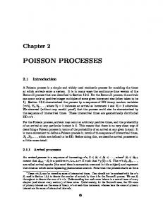
Optimal level of quality of service

100

50

A win-win incentive scheme

Incentive scheme for losses  Network losses do not represent a cost for the distribution utility (ohmic losses are a generation cost)  This is not a trivial matter, since network losses are a major driver for optimal network investment & a significant component of the cost of electricity  Since ohmic losses happen in distribution networks, regulation must incentivate operation & investment actions by distributors that account for losses efficiently 102

51

Incentive scheme for losses  The adequate regulatory scheme should mimic the one that has been described for quality of service  The reference revenue cap should be based on the current level of losses in the network  Add a penalty or a credit for deviations, in such a way that the company has an incentive to reduce losses up to the optimal level (which is also area specific, i.e. rural, urban, etc.)  So that consumers also benefit from this scheme  Network Reference Models (NRMs) can be used to determine the incentive factor  As with quality of service, simpler versions have been used 103 elsewhere

Distributed generation

A new regulatory context  Increased penetration of generation in distribution networks will require new forms of evaluation of the relationship between distribution costs & investments, losses & quality of service  Distribution grid operators are reluctant to enable largescale integration of generation facilities into their distribution grids, unless the corresponding extra cost drivers in this context are not understood, quantified & cost recovery is guaranteed  Network Reference Models may be useful here  Preliminary regulatory experience in the UK 106

52


Details

Negative incentives

 Contrary to transmission, distribution networks originally are not designed to accommodate generation  design, operation, control & regulation have to be adapted to allow potential massive deployment of DG  Under passive network management DG penetration generally results in additional costs of network investment & losses, an effect that increases with penetration levels  distribution utilities may be biased against DG & may create barriers to its deployment 107


Details

Need for advanced models

 Revised regulation of the distribution activity (DSO)  Refine the models of remuneration of distribution networks, so that the extra costs/benefits of accommodating DG & efficiency measures are recognized & negative incentives are minimized  Incentive-based regulation to reduce network losses & to improve quality of service, but now including DG in the scheme (e.g. adapting the performance indicators for losses & quality of service to the level of DG penetration)

 Find instruments to incorporate deployment of effective innovative technologies in the remuneration schemes 112


Details

Reference Network Models (RNM)

 A RNM is a network that minimizes the total cost of  Investment  O&M costs  Energy losses in the network

while meeting prescribed continuity of supply targets (or explicitly including the cost of non supplied energy) in the different supply areas (e.g. urban, suburban, concentrated rural, dispersed rural)

 RNMs may be used as an aide or benchmark (with any required adjustments) when  computing the revenue cap for the next period  designing incentive schemes for losses or quality of service

113

Case study: LV networks in Spain

Location of LV customers

Location of MV/LV transformers

57

Case study: LV networks in Spain

LV lines

Detail: An urban LV network Street map, LV and MV network, LV customers and MV/LV transformers

58

Non-technical distribution losses Illegal consumption of electricity

 Typically associated to situations of social margination  Measures usually taken when the situation has a negative & significant impact on the economic results of some firm or institution  Non discriminated power interruption is not a solution  It may affect consumers who pay  There is a potential willingness to pay that is wasted  A vicious circle: poor quality of service  no willingness to pay 117

Distribution regulation

PRICING

118

59

Pricing

The objective  Objective: To allocate the global remuneration of the distribution network to the individual users  Distribution charges are a component of  the “integral” tariff (for non-qualified consumers)  the “access” tariff (for qualified consumers)  Any charges to connected generators

 Distribution charges should  be cost reflective  completely recover the network costs 119

Pricing

Structure of distribution charges  Typical regulated distribution charges in the tariffs of most systems (only for demand)  Connection charge (€, paid only once): for a new connection to the network or the extension of an existing connection  Commercial charge (€, annual charge per type of customer): typically charged only to captive consumers; strictly not a distribution charge  Use-of-system charge (typically with an energy €/kWh & a capacity €/kW component): to recover the remaining distribution network total costs 120

60

Pricing

(distribution network tariffs)

Why not nodal prices?

 Most regulators prefer not to make distinctions between the distribution charges of identical consumers connected at different nodes in the distribution network  It seems that distribution nodal prices can be widely different in neighboring nodes & they may depend much on the flow patterns & the functioning of the technical devices in the network  This topic has not received much attention yet, although distributed generation has created the need for an in-depth analysis 121

Pricing


The procedure (just for demand)

 Split the network cost into the partial costs of the different voltage levels  Every consumer pays only the costs of its voltage level and upstream  Capacity charge ($/kW)  based on the coincidental peak demand

 Energy charge ($/kWh)  accounts for non peak consumption & besides, it is a proxy for peak demand for (small) consumers without adequate meters 122

61

Pricing


Some ideas (to include also generation)  It is becoming clearer the need to send locational & operation signals to potential & existing distributed generation  Locational connection charges for siting

 Based on the location of the generator in the distribution network & the need for reinforcements

 Network-related factors for remuneration of energy production  To incentivate production at times when local prices for energy or ancillary services are high, or emergency conditions may exist

123

Distribution regulation

ACCESS

124

62

Access

The objective Objective:  To establish the rules of use of the distribution network so that  no agent is discriminated  there is no abuse of the monopolistic power of the distributor

 To charge adequately for the facilities to connect to the network 125

Obligation of supply

(typically associated to supplier of last resort)  Service is mandatory to all existing & new users in the franchise area  Connection charges require specific regulation  new users  capacity expansions of existing users

 Access conditions require specific regulation  when network reinforcements are required  when access is required by competitors (depending on consumers´ choice capability) 126

63

Access  Representative cases

 Consumers directly connected to a distribution network  and supplied by it  and supplied by an independent retailer

 Generators directly connected to a distribution network  selling the power to this distributor  selling the power elsewhere

 Wholesale transactions using a distribution network and involving:  other distribution utility  a directly connected eligible consumer  a directly connected generator

127

Access

Conflicts with access rights  Basic principles  Universal right to connection  Incurred costs must be born by network users  Access rights are independent of choice of retailer

 The regulator will solve any existing conflicts  abuses of dominant position  lack of definition of territorial franchises  Discrimination of small distributors with respect to other clients of its supplier & to clients that are served by other suppliers 128

64

Access

Conflicts with connection charges  Should the cost of every connection be individualized?  uniform charge up to a threshold  individualized charges beyond

 Physical construction of connections should not be a monopoly of the incumbent distributor  minimum design & operational requirements 129

Obligation of supply RURAL ELECTRIFICATION  Some rural areas may lack electricity supply  The cost of supply in these areas typically far exceeds the average distribution cost  decentralized systems with local generation may be the best option  The risk of no payment may also be higher than average  Some ad hoc scheme is needed to develop distribution networks to these areas  Subsidies from the Government will be needed  Desirable to involve private interests  Use market mechanisms for assignment of subsidies whenever possible  Avoid dependency from subsidies: assign just once 131

65

Rural electrification Case example (Chile)  Governmental agency issues a request for proposals each year, indicating the total amount of subsidies to be awarded  Selection criteria: maximize the social impact of subsidy: largest number of connections & lowest cost for end user  The subsidy turns unattractive projects for the private firms into attractive ones  Once built, the new facilities must be treated as any other distribution facility of the winning firm

132

66

Engineering, Economics & Regulation of the Electric Power Sector ESD.934, 6.974

Sessions 5 & 6 Module C. Part 2 (recitation)

Electricity distribution & the regulation of monopolies Prof. Ignacio J. Pérez-Arriaga

Annex

The role of network reference models (NRM) in electricity distribution regulation

1

Regulatory instruments  In each price review the regulator basically uses two kinds of instruments to help in the estimation of the future costs of the firm & to reduce the problem of information asymmetry  Regulatory accounting systems (historic record of OPEX, investment, and DSO assets)

 Models to estimate the network costs

(benchmarking or network reference models)

3

Case example

Spain

(Royal Decree RD 222/2008)

 The new regulatory scheme establishes incentives for

 Efficient investment to meet demand increments & new connections  Improvements in continuity of supply  Network loss reductions

 Information asymmetry is mitigated by the use of  Regulatory accounting  Network reference models

 Network reference models provide a benchmark for investment and O&M costs, while taking into account continuity of supply requirements and network loss reduction targets 4

2

Network reference models (NRM)  NRM is a network that minimizes the total cost of  Investment  O&M costs  Energy losses in the network

while meeting prescribed continuity of supply targets (or explicitly including the cost of non supplied energy) in the different supply areas (e.g. urban, suburban, concentrated rural, dispersed rural)

 NRMs may be used as an aide or benchmark (with any required adjustments) when  computing the revenue cap for the next period  designing incentive schemes for losses or quality of service

5

Network reference models (NRM)  Network reference models can be used as:  Greenfield models: An efficient distribution network is developed from scratch, starting from the GPS location & demand of consumers and the location of transmission substations  Assessing utility’s network technical efficiency as a benchmark of actual networks  Development of networks in the long-term under technological uncertainty (Smart-grids paradigm)

6

3

Network reference models (NRM)  Network reference models can be also used as:  Incremental models: The model efficiently reinforces the existing network to address estimated demand increments and new connections during the price control period  Network reinforcements in the short and medium-term  Analysis of costs/benefits of DG penetration, response demand actions, or energy efficiency programs

7

Network reference models (NRM)  Since the data to perform benchmarking are frequently not available  NRMs are an interesting alternative  Their purpose is NOT to micromanage the distribution company, but  To reduce the lack of information of the regulator  To provide sound numerical values for some incentive schemes (e.g. losses, quality of service)

 Network reference models have been used in Argentina, Chile, Spain or Sweden 8

4

Network reference models (NRM)  Elements of the planning function  Capital expenditure (CAPEX)  Costs of building the network

 Operational expenditure (OPEX)  Operation & Maintenance costs of the network

9

Capital expenditures (CAPEX)  Electricity networks are very intensive in capital investment  New customers connections  Investment in new network installations  Upgrade of old installations

5

Operation Expenditures (OPEX)  Operational expenditures (OPEX)  Maintenance of the elements of the networks  Operation of the network

 Highly correlated to the CAPEX  Almost no “variable cost”: it doesn’t depend on the level of utilization of the network  Once the CAPEX is known (along with its characteristics), the OPEX can be determined (assuming an efficiency level)

Planning function  To understand the CAPEX, we need to understand the network planning function  Minimize {investment + losses + OPEX} Subject to:  Capacity (load requirements)  Quality (Power quality and continuity of supply)  Geography (location of customers, geographical constraints)

 The planning function determines the cost function

6

Description of an actual NRM • Large scale ( > 1 million customers) • Both urban & rural areas • Detailed Geographical Features: • Settlements identification • Automatic street map building • Forbidden ways through • Aerial/underground areas • Voltage, capacity & reliability constraints • Detailed standardized equipment and parameter library • Detailed reliability assessment

Reference: J. Román, T. Gomez, A. Muñoz, J. Peco, "Regulation of distribution network business," IEEE Transactions on Power Delivery. vol. 14, no. 2, pp. 662-669, April 1999.

NRM: hierarchical structure Network Structure

Types and number of facilities Transmission substations HV network

(36, 220) kV

HV/MV substations MV network

> 150

(1, 36) kV

MV/LV transformers LV network

> 15

> 15000

< 1kV LV customers

> 106

•  Input Data: HV, MV and LV customers, and transmission substations • Results of the model: LV, MV & HV network, HV/MV and MV/LV substations

7

15

16

8

17

The picture shown on the right depicts the outlines of the settlements in red. These outlines represent the frontier between the network affected by orography, forbidden ways through... and the network constrained by the 18 street maps.

9

LV network

Data & MV/LV transformers

Location of LV customers

Location of MV/LV transformers

10

LV network

LV lines

11

MV urban network

Urban LV network Detail of street map, LV and MV network, LV customers and MV/LV transformers

12

MV urban/rural network HV/MV substation Network loops

MV feeder

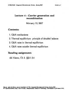
Application of NRM: incremental costs as a function of demand

fe = 0.55

13

MIT OpenCourseWare http://ocw.mit.edu

ESD.934 / 6.695 / 15.032J / ESD.162 / 6.974 Engineering, Economics and Regulation of the Electric Power Sector Spring 2010

For information about citing these materials or our Terms of Use, visit: http://ocw.mit.edu/terms.