Topographically specific functional connectivity ...

NeuroImage 56 (2011) 1426–1436

Contents lists available at ScienceDirect

NeuroImage j o u r n a l h o m e p a g e : w w w. e l s e v i e r. c o m / l o c a t e / y n i m g

Topographically specific functional connectivity between visual field maps in the human brain Jakob Heinzle a,⁎, Thorsten Kahnt a,b, John-Dylan Haynes a,b,c,⁎ a b c

Bernstein Center for Computational Neuroscience, Charité–Universitätsmedizin Berlin, Germany Berlin School of Mind and Brain, Humboldt–Universität zu Berlin, Germany Max Planck Institute for Human Cognitive and Brain Sciences, Leipzig, Germany

a r t i c l e

i n f o

Article history: Received 23 November 2010 Revised 26 January 2011 Accepted 27 February 2011 Available online 3 March 2011

a b s t r a c t Neural activity in mammalian brains exhibits large spontaneous fluctuations whose structure reveals the intrinsic functional connectivity of the brain on many spatial and temporal scales. Between remote brain regions, spontaneous activity is organized into large-scale functional networks. To date, it has remained unclear whether the intrinsic functional connectivity between brain regions scales down to the fine detail of anatomical connections, for example the fine-grained topographic connectivity structure in visual cortex. Here, we show that fMRI signal fluctuations reveal a detailed retinotopically organized functional connectivity structure between the visual field maps of remote areas of the human visual cortex. The structured coherent fluctuations were even preserved in complete darkness when all visual input was removed. While the topographic connectivity structure was clearly visible in within hemisphere connections, the between hemisphere connectivity structure differs for representations along the vertical and horizontal meridian respectively. These results suggest a tight link between spontaneous neural activity and the fine-grained topographic connectivity pattern of the human brain. Thus, intrinsic functional connectivity reflects the detailed connectivity structure of the cortex at a fine spatial scale. It might thus be a valuable tool to complement anatomical studies of the human connectome, which is one of the keys to understand the functioning of the human brain. © 2011 Elsevier Inc. All rights reserved.

Introduction Neurons in the mammalian brain exhibit a large degree of ongoing activity. This spontaneous activity can be observed independent of any sensory input or motor activity. Spontaneous fluctuations are observed on many spatial and temporal scales (Arieli et al., 1996; Fiser et al., 2004; Fox and Raichle, 2007; He et al., 2008, 2010). Importantly, the intrinsic functional connectivity of cortex can be measured by the correlation structure in spontaneous fluctuations. It has been suggested that the underlying anatomical architecture of the central nervous system shapes the spatial pattern of the intrinsic functional connectivity. At a fine spatial scale, spontaneous activity has a strong influence on local cortical sensory processing (Arieli et al., 1996; Fiser et al., 2004), and the local intrinsic functional architecture is highly specific and closely matches the functional architecture of visual cortex acquired from sensory evoked activity (Tsodyks et al., 1999). However, it is not known whether such detailed influences are ⁎ Corresponding authors at: Bernstein Center for Computational Neuroscience, Philippstr. 13/Haus 6, D-10115 Berlin, Germany. Fax: +49 30 2093 6771. E-mail addresses: [email protected] (J. Heinzle), [email protected] (J.-D. Haynes). 1053-8119/$ – see front matter © 2011 Elsevier Inc. All rights reserved. doi:10.1016/j.neuroimage.2011.02.077

restricted to local cortical circuits or whether a detailed functional connectivity would be evident also if signals from distant cortical regions are considered. At a coarse spatial scale, there is a large-scale inter-regional correlation structure in the intrinsic functional connectivity of the brain which is evident in spontaneous activity measured with fMRI (Biswal et al., 1995; Fox and Raichle, 2007; Nir et al., 2006; van den Heuvel and Hulshoff Pol, 2010; Vincent et al., 2007; Wang et al., 2008; Zou et al., 2009). Importantly, the functional long-range interactions have been related to large white matter tracts (Greicius et al., 2009; Hagmann et al., 2008; Honey et al., 2009) and follow the known anatomical connectivity patterns in monkeys (Margulies et al., 2009). Based on these findings, intrinsic functional connectivity measured with fMRI was suggested as a ‘tool for human connectomics’ (Van Dijk et al., 2010). The anatomical connectivity of cortex has been studied on several scales as well. For an overview see Douglas and Martin (2004). On the large scale, cortical connections have mostly been characterized by areal counts of labeled neurons (see e.g., Fellemann and van Essen, 1991). In recent years, diffusion tensor imaging has been employed to measure large axonal bundles between cortical regions in vivo in humans (e.g. Hagmann et al., 2008). On the fine scale, the detailed local cortical microcircuit has been characterized only in few cortical

J. Heinzle et al. / NeuroImage 56 (2011) 1426–1436

areas and species, for example in cat visual cortex (Binzegger et al., 2004). Further, it has been shown that the distribution of local, horizontal connections is related to functional maps (Bosking et al., 1997), suggesting a tight link between function and local anatomy. Despite the long history of anatomical studies, relatively little is known about how inter-areal anatomical connections precisely align with cortical topographies, in general. However, a visuotopic anatomical connectivity has been demonstrated between visual areas in the monkey (Angelucci et al., 2002; Salin and Bullier, 1995). Importantly, a large fraction of the synapses onto a cortical neuron are of local origin (Binzegger et al., 2004), while only relatively few synapses are connections from distant cortical areas. This large number of local connections provides the basis for the tight link between spontaneous and evoked activity in local circuits (Tsodyks et al., 1999). However, it is not known whether the relatively few synaptic connections between cortical areas might suffice to shape spontaneous fluctuations in a fine detailed manner even across cortical regions. For example, the intrinsic functional connectivity between topographically organized visual areas might be related to the detailed retinotopic functional organization of the two regions, similar to the anatomical connections in the monkey (Salin and Bullier, 1995). Here, we used fMRI to measure the fine-grained functional connectivity structure between different topographically organized regions of the human visual cortex. In analogy to visual receptive fields (Dumoulin and Wandell, 2008; Hubel and Wiesel, 1968), we estimate cortico-cortical receptive fields (CCRF) between visual areas V1 and V3, which were then averaged to obtain the topographic connectivity structure (TCS) between the two retinotopic maps. The specific term CCRF of a neuron, or voxel in our case, is in accordance with the concept of a cortical projective field (Sejnowski, 2006). Importantly, we measured the TCS under two fundamentally different conditions: with visual stimulation and without any visual input. The second condition is of particular interest, because the resulting TCS shows the intrinsic functional connectivity and is very likely to reflect the underlying anatomical connectivity. Importantly, the use of fMRI allows us to simultaneously measure activity in distinct topographically organized maps and directly estimating their functional interactions. Materials and methods To characterize the spatial structure of functional connectivity between two visual field maps, we measured the linear, spatial filter in a lower visual area (V1) that best predicted activity of a voxel in a higher visual area (V3). In analogy to visual receptive fields (Dumoulin and Wandell, 2008; Hubel and Wiesel, 1968), these topographic connectivity patterns can be regarded as cortico-cortical receptive fields (CCRF, see Fig. 1A). The CCRF were estimated for all voxels in V3 and then averaged to obtain the average CCRF, i.e. the topographic connectivity structure (TCS) between the two retinotopic maps. First, we measured the visually evoked TCS, while subjects watched a checkerboard stimulus with randomly flickering segments. Second, in order to reveal the intrinsic functional connectivity structure reflected in spontaneous activity, we scanned subjects without any visual input. The individual steps of the analysis are described in detail below. Participants Eight right-handed, healthy subjects (three females, age range 24– 34 years) participated in the experiments. All subjects had normal or corrected to normal vision and gave written informed consent to participate in the fMRI experiment. The experiment was approved by the local ethics review board of the Max Planck Institute for Human Cognitive and Brain Science (Leipzig) and conducted according to the Declaration of Helsinki.

1427

Experimental design Four subjects participated in three scanning sessions: A retinotopic mapping experiment, a purely visual experiment (S+) and a resting state experiment without any visual stimulation (S−). The four other subjects participated only in S− and retinotopic mapping experiments. In the two visual experiments (S+ and retinotopic mapping) subjects were engaged in a fixation task (Landolt C) at the center of the visual display. Visual stimuli were projected onto a translucent screen at the rear of the scanner (screen size: 25° by 20° of visual angle). During S+, subjects were presented with 8 runs of a high contrast, flickering circular checkerboard subdivided into 48 segments which changed their local contrast (4 logarithmic levels between 0.1 and 1) independently over time (Fig. 2). Note that the visual stimulus had a border along the vertical meridian resulting in completely independent visual stimulation in the two visual hemifields. In S−, subjects were asked to keep their eyes closed during the whole experiment. To minimize confounds from possible eye openings, subjects wore a blindfold and the scanner room was completely darkened by covering all light sources within the room. fMRI image acquisition Standard functional EPI images were acquired on a 3-T Siemens Trio (Erlangen, Germany) with a 12-channel head coil. In S+ and S−, runs consisted of 220 T2*-weighted gradient-echo echo-planar images (EPI): TR = 1500 ms, TE = 30 ms, flip angle = 90°, matrix size = 64 × 64, field of view (FOV) = 192 mm, 25 slices (2 mm thick, 1 mm gap, ascending) resulting in a voxel size of 3 by 3 by 3 mm. In retinotopic mapping runs, 160 T2*-weighted volumes with 33 slices were acquired (TR = 2000 ms, all other parameters equal as above). A whole-brain EPI image (parameters as above but with 70 slices, TR = 4300 ms) was collected after each session as well as a T1weighted structural data set with 1 mm3 resolution (TR = 1900 ms, TE = 2.52 ms, matrix size = 256 × 256, FOV = 256 mm, 192 slices of 1 mm thickness, flip angle = 9°). Data preprocessing Images were slice time corrected, realigned and coregistered to the anatomical image of each subject using SPM2 (Wellcome Department of Imaging Neuroscience, Institute of Neurology, London, UK). First, all functional images were coregistered to the whole-brain EPI image within scanning session, then the whole-brain EPI was coregistered to the anatomical image and the transformation parameters were applied to all functional images. Finally, the data from V1 and V3 was extracted using the masks obtained by standard retinotopic mapping (see below). Ten volumes at the beginning and at the end of each run were discarded, resulting in runs of 200 volumes each that entered the connectivity analysis. Raw time courses were corrected for movement parameters, the global mean over the whole brain and a linear trend. Note that the correction for the global mean has been demonstrated to remove most of the physiological noise due to breathing and heart rate modulations (Van Dijk et al., 2010). SVR training and prediction We analyzed each data set separately with a support vector regression (SVR) using a leave one out cross-validation procedure. A standard linear SVR (ε-SVR, LibSVM, www.csie.ntu.edu.tw/~cjlin/ libsvm) was trained on the raw data in V1 of 7 out of 8 runs to predict the time courses of voxels in V3. The parameter ε controls the sparseness of the SVR and was set to 0.1, a level at which most of the data points were retained as support vectors (C = 0.01). Prior to the SVR analysis, the raw data in every voxel (in V1 and V3) was z-normalized to zero mean and unit standard deviation separately for the training and test

1428

J. Heinzle et al. / NeuroImage 56 (2011) 1426–1436

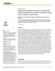
Fig. 1. The concept of cortico-cortical receptive fields. (A) In analogy to a visual receptive field (left, yellow) cortico-cortical receptive fields (CCRF; right, blue) are defined as the spatial filter within a lower visual area (V1) that best predicts the activity in a higher visual area (V3). (B) Four sample CCRFs, for four different voxels of V3, are sketched on top. Note the different positions of the dashed white lines and black circles that indicate the retinotopic position of the corresponding V3 voxel. The individual CCRFs are overlaid in the coordinate frame defined by the white lines and then averaged to obtain the average topographic connectivity structure (TCS). Arrows indicate the position of individual CCRFs within the TCS. Please note that the spatial alignment used for averaging is based on the independent retinotopic mapping data and not on the results of the S+ or S− experiment. (C) The CCRF of a voxel is given by the weight distribution of the optimal linear combination of voxels in V1 (yellow) that best predicts the signal fluctuations of a voxel in V3 (blue). An example CCRF is shown below. The left shows V1 and dorsal V3 in cortical space (CS). The position of the predicted V3 voxel is shown by the white dot. The weights of individual V1 voxels are indicated by different colors. The right shows the same map transformed from cortical space to Cartesian retinotopic space (CRS) and polar retinotopic mapping space (PRS). White dashed lines indicate retinotopic mapping coordinates (α: visual angle (azimuth), r: visual eccentricity). The prediction accuracy (correlation between the predicted and measured time course of the V3 voxel) captures how well the CCRF predicts the activity in V3.

data set. We trained a separate SVR for every voxel in V3, always using the raw fMRI traces of all voxels in V1 as the input. The distributions of the weights in V1 define a spatial filter on V1 that predicts an individual voxel's time course in V3. Hence, the prediction V3,j(t) of the activity of the jth voxel in V3 is given by n

V3; j ðt Þ = ∑ wji V1;i ðt Þ; i=1

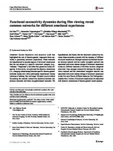
Fig. 2. Visual stimulation paradigm.During S+, subjects viewed a flickering checkerboard, while fixating on the center of the screen. Four sample checkerboards are shown. The checkerboards flickered at a frequency of 10 Hz and were subdivided into 48 segments that changed their local contrast independently over time using M-sequences. The contrast pattern changed (between 4 levels) every 3 s. The dashed and dotted lines on top illustrate the local contrast (numbers indicate contrast levels) of two sample segments over time, surrounded by the dashed line and dotted line respectively. Each of the 8 runs of experiment S+ consisted of a series of 100 checkerboards (run duration: 300 s).

ð1Þ

where V1, i(t) are the time-courses for all n voxels in V1 and wji are the weights estimated by the SVR on the trainings runs. The CCRFs were calculated within hemispheres as well as between hemispheres. The prediction accuracy for each SVR was assessed using data that was not used to train the SVR. Specifically, the average prediction accuracy is given by Fisher's Z-transformed correlation between the predicted and measured time courses of the V3 voxel in the 8th run. Importantly, this cross-validation procedure assures that the reported correlations coefficients are true predictions and not due to overfitting, which could happen due to the large number of voxels in V1. Please note that similar results would be obtained using a slightly less efficient multiple linear regression approach.

J. Heinzle et al. / NeuroImage 56 (2011) 1426–1436

Calculating the topographic connectivity structure as average CCRFs The weight maps for each SVR were transformed from cortical space to polar retinotopic space based on the retinotopic mapping (Fig. 1C), aligned relative to the position of the V3 voxel in visual space (for between hemispheres CCRFs we used as a reference the retinotopic mapping coordinates of the V3 voxel mirrored at the vertical meridian), and interpolated on a grid (200 by 200 points) ranging from −π to π for both angular and eccentricity phase values. Finally, all maps were averaged, yielding the TCS between V1 and V3 (Fig. 1B). Note that the TCS is given in relative (between V3 and V1) coordinates: Δα and Δr. For the visual stimulation paradigm (S+), the statistical significance of these TCS was assessed by randomly permuting the association between weight maps and V3 voxel positions 1000 times and identifying the parts of the connectivity structure, where the true map was higher than all random maps, resulting in a significance level of p b 0.001. To quantify how well retinotopy was conserved in the S− experiment, we calculated the mean of the weight structure within a central disk and subtracted from it the mean in an annulus of the same radius. The size of the central disc was chosen to match the size of the significant regions in S+. We then tested whether (1) the difference between center and surround was significant (one sample t-test) and whether (2) this effect was significantly stronger in the within hemisphere condition than in the between hemisphere condition (paired t-test). All statistical tests were performed over the 8 subjects (resp. 4 in S+). For this, the within hemisphere and between hemisphere maps were averaged within each subject, yielding two respective maps for each subject. We also calculated the mean of the connectivity weights as a function of distance from the center of the TCS. Finally, in order to illustrate the dependency of the TCS on the visual angle and the eccentricity separately, we averaged the TCS over each of the two variables within a central range of Δα=[−π/5, π/5] and Δr=[−π/5, π/5] respectively. We report all results by the mean ±s.e.m. over subjects (n=8). Finally, we verified whether the prediction of the time course of V3 voxels was better when we restricted the voxels in V1 to those with similar representations in the visual field, compared to voxels with a different visual field representation. Based on the independent retinotopic mapping, we selected for each voxel in V3 the 50 voxel in V1 that had their visual field representation closest to the V3 voxel. For the selection of voxels in V1 we used the distance Δ in polar qffiffiffiffiffiffiffiffiffiffiffiffiffiffiffiffiffiffiffiffiffiffiffiffiffiffiffiffiffiffiffiffi coordinates (Δ =

ðΔαÞ2 + ðΔr Þ2 ). We then predicted the time

course of the V3 voxels using those 50 voxels with exactly the same SVR analysis as described above. The same procedure was repeated for the 50 voxels with their visual field representations farthest away from the V3 voxel. The difference in mean prediction accuracy (mean over all V3 voxels in every subject) between the two predictions was tested against the hypothesis of no difference using a t-test across subjects (n = 8) on the Fisher's Z-transformed correlation coefficients.

Retinotopic mapping and selection of V1 and V3 ROIs Retinotopic mapping was performed using a standard traveling wave method with a double wedge and an expanding ring stimulus (Wandell et al., 2007; Warnking et al., 2002). In this setting angular phase values range from 0 to 2π within each hemisphere and are directly proportional to the azimuth spanning the 180° of one visual hemifield. The eccentricity of the expanding rings was chosen so that the eccentricity phase r (also ranging from 0 to 2π) was proportional to log(1 + ecc), where ecc is the eccentricity in degrees of visual angle. Note that this choice of the size of expanding rings takes into account cortical magnification (Engel et al., 1997) and assures that differences in the phase r are approximately linear to cortical distance. Six runs (4 for visual angle and 2 for eccentricity mapping) of 150 images were

1429

collected. We used FreeSurfer for gray matter segmentation of the anatomical images (Dale et al., 1999) and mrGray for cortical flattening (Wandell et al., 2000). In house software using Matlab (The MathWorks, Natick, MA) was used to generate the flattened angular and eccentricity maps. Based on the angular map, we defined by visual inspection the borders between early visual areas V1, V2 and V3. The ROIs for the visual areas V1 and V3 were defined based on these borders on the flattened surface, transformed back to 3-dimensional anatomical space and then to the functional image space of the EPI images. Comparing CCRF predictions to a mean model The prediction accuracies obtained from comparing the predicted and observed V3 time courses allow us to compare predictions from different models. In order to assess the contribution of the detailed structure of the CCRFs to the prediction accuracy, we compared the CCRF predictions to predictions based on a simpler model that predicted activity of individual voxels in V3 from the mean activity in V1. This “Mean”-model does not include any information that can be gained from the spatial structure of the connections and reflects the connectivity only on a coarse level, averaging over large cortical regions. The time course of the jth voxel in V3 V3, j(t) was predicted by the mean activity in V1, and therefore V3;j ðt Þ =

1 n ∑ V ðt Þ: n i = 1 1;i

ð2Þ

Note that this is equivalent to the predictions of the CCRF, but with all weights equal to 1/n. Like the CCRF predictions, ‘Mean’ predictions were calculated for every run and voxel individually. Hence, the results of the two analyses can be directly compared. For each subject we calculated the average prediction accuracy (based on Fisher's Ztransformed correlations) for both stimulation conditions S+ and S− within as well as between hemispheres. The resulting accuracies of the CCRF and ‘Mean’ predictions were compared by paired t-tests (n = 4 in S+, n = 8 in S−). Testing for effects of cortical distance We have deliberately chosen V1 and V3 for our analysis in order to exclude possible confounds due to shared vasculature or cortical distance. If we had taken V2 instead of V3, many voxels in the two regions would have been immediate spatial neighbors while also sharing the same retinotopic representation. Hence, the relatively longrange interactions (up to 1 cm) of LFP fluctuations (Leopold et al., 2003) will cause an overestimation of retinotopic functional connectivity if measured between V1 and V2. Due to the functional organization of early visual cortex this confound is absent between V1 and V3. In order to empirically confirm that the observed TCS did not depend on cortical distance, we conducted the very same analysis as for the functional TCS, but with the Euclidian distance between V3 voxels and V1 instead of the SVR weights. The same statistical tests that were used for experiment S− served to show that there is no significant effect of distance that could contribute to the TCS. Results The presentation of the results will focus on the final result of the detailed analysis, i.e. the topographic connectivity structure between retinotopic maps. We will first present the results from experiment S+, where we observe a clear retinotopic structure in line with the visual stimulation. Then the intrinsic TCS measured without any visual input (S−) is presented in detail. The topographic specificity of the TCS is illustrated by several additional analyses, and finally, we compare the predictions of the CCRF to a simpler model and also exclude that the observed structure is merely due a distance effect.

1430

J. Heinzle et al. / NeuroImage 56 (2011) 1426–1436

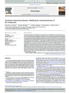
Topographic connectivity structure during visual stimulation The connectivity structure between V1 and V3 was first measured for 4 of the 8 subjects under visual stimulation. The visual stimulation consisted of a flickering polar checkerboard that changed its local contrast independently over time in 48 segments (Fig. 2). We then estimated the topographic connectivity structure between V1 and V3. In the TCS, parts of V1 that are associated with high weights contribute strongly to the prediction of activity in V3, while regions with lower weights are less important for the prediction. We find that the within hemisphere TCS measured in individual subjects under visual stimulation clearly reflect the retinotopic organization (Fig. 3A). As a control we also estimated the TCS between hemispheres, i.e. predicting time courses of voxels in the left V3 from activity in the right V1 and accordingly for the right V3. Importantly, no structure was observed in these maps calculated between hemispheres, providing evidence for the specificity of this structure for within hemisphere connections. In order to ensure that the retinotopically specific co-fluctuation we found between V1

and V3 was not simply the mere result of the averaging procedure, we performed a random permutation testing which shows that the TCS within hemispheres have significantly higher weights (p b 0.001) than expected by chance between parts of V1 and V3 that represent the same retinotopic position. This specific pattern was consistently observed in all 8 hemispheres (2 hemispheres in 4 subjects) illustrating that, during visual stimulation, regions with similar retinotopic representations in the two visual field maps are functionally connected. Fig. 3C depicts areas with significant weights for all 4 subjects. In a further step, we characterized to which degree the observed TCS are visuotopically organized. Fig. 3B depicts the average TCS over all 8 hemispheres. Based on this map, we calculated the average weight within the TCS as a function of the distance from the center of the TCS (Fig. 3D). In accordance with the classical feed-forward model, the weights of the TCS are high around the center of the TCS and low in the periphery. Thus, ongoing visual activity in V3 is best predicted by parts of V1 that correspond to a similar position in the visual field. Supplementary Figure S1 shows examples of CCRFs of two individual voxels. The prediction of raw time courses of V3 voxels was significant within hemispheres (rwh = 0.21 ± 0.02, Fisher's Z-transformed average accuracy ± s.e.m., 4 subjects). Note that although not the entire variance of the raw time courses is explained by the SVR model (probably due to the high noise level of fMRI signals), this result is highly significant. Importantly, within hemisphere predictions were significantly higher than between hemisphere predictions (rbh = 0.16 ± 0.02, p = 0.009, paired t-test). Compare also Table 1.

Topographically organized connectivity in absence of visual input

Fig. 3. Topographic connectivity structure under visual stimulation. (A) The TCS of a single subject (Sub 4) are shown for the within hemisphere (wh, top row, left V1→left V3, right V1→right V3) and the between hemisphere condition (bh, bottom row, left V1→right V3, right V1→left V3). Weights are color-coded (see color bar below) between the lowest and highest weight over both TCS. (A) Average TCS over all 4 subjects (8 hemispheres) for within hemisphere (top) and between hemisphere conditions (bottom). Weights are color-coded (see color bar in A) between the lowest and highest weight over both average TCS. (C) A permutation test was used to extract regions that have significantly higher weights (p b 0.001) than any of 1000 random TCS. The largest closed significance contour of each within hemisphere TCS (n = 8) is shown here for the within hemisphere TCS. Contours are plotted with a different color for each subject (see insets, 2 contours per subject). Note that all significant regions are located around the center of the TCS. (D) Average weights (over 4 subjects) as a function of distance from the center of the TCS. Note that the within hemisphere TCS (solid line) exhibits a clear gradual decrease of weight with increasing distance from the TCS center. This finding is highly significant (shaded areas indicate s.e.m.). The dashed line indicates TCS between hemispheres (s.e.m. indicated by shaded area).

In order to test whether the observed visuotopy was a mere result of visual stimulation or actually reflects the underlying fine-grained architecture of cortico-cortical connections, we performed a second experiment and measured the TCS for spontaneous brain activity. All 8 subjects were scanned with the same scanning parameters as in S+ but without any visual stimulation (S−). Subjects were blindfolded and asked to keep their eyes closed during the entire scanning session. Importantly, we performed exactly the same analysis steps as for the visual stimulation experiment S+. Even without any visual input, time courses in V3 voxels are significantly predicted within hemispheres (rwh = 0.21 ± 0.02, Fisher's Z-transformed average accuracy ± s.e.m., 8 subjects). As under visual stimulation, the predictions were again significantly higher within than between hemispheres (rbh = 0.19 ± 0.02; p = 0.001, paired t-test, see also Table 1). Notably, also in the second experiment (S−) the TCS within hemispheres is clearly retinotopically organized, even though it was measured in the absence of any visual input. Fig. 4 shows the TCS of a sample subject and the average TCS over all subjects (compare also Supplementary Figure S1 for example CCRFs of individual voxels). Again, the illustration of the average weight as a function of the distance of the TCS center clearly reveals a retinotopic organization of the connectivity structure (Fig. 4C). Even in the absence of any visual stimulation, the weights in the center are highest and gradually decrease with distance from the center. Thus the TCS likely reflects the underlying connectivity structure between V1 and V3. In order to statistically verify the retinotopic organization of the TCS in spontaneous fluctuations, we calculated the difference between a center and a surround region in the connectivity map. Importantly, the size of the central region was defined from the previous S+ experiment (compare Fig. 3C). This assured that all parameters entering the analysis of S− data were completely independent of the data itself. The center– surround difference is highly significant (p b 0.001, one sample t-test) and higher within than between hemispheres (p b 0.01, paired t-test) (Fig. 4D), conclusively demonstrating that the presence of TCS does not depend on visual stimulation.

J. Heinzle et al. / NeuroImage 56 (2011) 1426–1436

1431

V3 around both Δα = 0 and Δr = 0. Hence, intrinsic functional connections are strongest between parts of the two visual maps that have similar representations in the visual field. Based on these results, we conclude that the TCS is likely to directly reflect the underlying visuotopic anatomical connections. We finally confirmed the retinotopic structure by comparing the within hemisphere prediction of the V3 time courses based on voxels in V1 that represent a similar position in visual space with the within hemisphere predictions based on voxels in V1 that have representations far away in the visual field. The predictions are significantly better (p = 0.002, t-test over subjects, n = 8) if based on voxels with similar visual field representation, further corroborating our finding of a topographic TCS between V1 and V3. Between hemisphere topographic connectivity along the vertical meridian

Fig. 4. Topographic connectivity structure without visual stimulation. TCS from experiment S−, without any visual stimulation. During scanning, subjects were blindfolded and had their eyes closed. (A) The TCS of a single subject (Sub 4) are shown for the within hemisphere (wh, top row) and the between hemisphere condition (bh, bottom row). Weights are color-coded (see color bar below) between the lowest and highest weight over both TCS. See Fig. 3A for detailed legend. (B) Average TCS (over all 8 subjects, 16 hemispheres) from experiments without any visual stimulation for within hemisphere (wh, top) and between hemisphere (bh, bottom) predictions. Weights are color-coded from lowest to highest using the same scaling in both maps. (C) Average weights as a function of distance from the center of the TCS. Note that the within hemisphere TCS (solid blue line) exhibit a clear gradual decrease of weight with increasing distance even without any visual input (S−). Please note that even for the S− condition this finding is highly significant. The respective curve for the S+ condition is shown in red for illustration (same as in Fig. 3D, but without s.e.m.). Dashed lines indicate CCRFs between hemispheres (red: S+, blue: S−). Shaded areas indicate s.e.m. over subjects (n = 8) for the S− experiment. (D) The difference between the weights in a central region (green dashed circle in inset on the right) and its surround (purple dashed circle) is a measure of how well retinotopy is conserved. To verify the retinotopic organization of functional connectivity in spontaneous fluctuations, the size of the central regions was based roughly on the size of the significant regions of the maps of all subjects in the S+ experiment (light gray curves, see Fig. 3C), thus excluding the possibility of any bias due to double-dipping. The center– surround difference of the weights is shown for the S+ (red bars; shown for illustration only) and S− (blue bars) experiments. Without visual input, the center–surround difference is significant in the within hemisphere condition (S−: p b 0.001) and higher in the within hemisphere compared to the between hemisphere condition (S−: p b 0.01). Note that because the binning of data for this specific figure was based on the results of the S+ experiment, a test of the statistical significance for the S+ condition would be meaningless. The between hemisphere TCS shows a slightly significant (p b 0.05, one sample t-test) weight difference between center and surround, which is completely due to a preference of high weights for similar eccentricity, but not visual angle (compare also Fig. 5). Bars show the mean C–S over all subjects (S+: n = 4; S−: n = 8) and error bars indicate s.e.m.

In Fig. 5, the structured functional connectivity is further illustrated by showing the TCS of all individual subjects. Based on these individual maps, we also assessed how the weights depend on the visual angle α and the eccentricity r, respectively (Fig. 5B and C). Finally, Fig. 5D summarizes this analysis and clearly demonstrates that the within hemisphere TCS shows a preference for high weights between V1 and

In an additional analysis, we assessed whether there are differences in the TCS for voxels in V3 around the horizontal meridian compared to the vertical meridian. We therefore, split the set of voxels in V3 into two groups, voxels with a visual field representation within 45° of the horizontal meridian and voxels with a visual field representation within 45° of the vertical meridian. Note that this splitting was performed based on the independent retinotopic mapping. We then performed the averaging procedure (compare Fig. 1B) that yielded the TCS individually for these two sets of V3 voxels (Fig. 6B). The same statistical analyses as for the entire visual field were used. Fig. 6 summarizes these interesting results. Along the horizontal meridian, the within hemisphere TCS is retinotopic, while there is clearly no topographic structure in the intrinsic functional connections between hemispheres (Fig. 6C). The center–surround difference is clearly significant within hemispheres (pb 0.01, one sample t-test) and higher within than between hemispheres (pb 0.01, paired t-test). This picture changes dramatically when the between hemisphere TCS is considered along the vertical meridian. Here, we observe a topographic functional connectivity between V1 and V3 on the other hemisphere as well (Fig. 6C). The center–surround difference (Fig. 6D) is clearly significant within hemispheres (p b 0.001, one sample t-test), but also in the between hemisphere TCS (pb 0.01). There is no significant difference between within and between hemispheres (pN 0.1, paired t-test). Interestingly, the difference between the vertical and horizontal meridian representations is much more emphasized for the experiment without visual stimulation. This is most likely a result of the visual stimulation which was statistically independent for the left and right visual hemifield and had a sharp border along the vertical meridian. Thus, neighboring voxel representing positions slightly left and right of the vertical meridian were stimulated differently in the S+ experiment. Comparison to ‘Mean’-model An alternative to the detailed CCRF prediction learned by the SVR is given by a simpler mean-model that tries to predict the activity of single voxels in V3 from the mean over all voxels in V1. We compared the predictions from such a mean-model to the CCRF predictions. Table 1 summarizes the results from this analysis. Predictions of single voxel time courses in V3 that are based on the detailed spatial connectivity structure learned by the SVR (CCRF) are significantly higher than predictions that are based on the mean activity within area V1 (Mean). The predictions based on the CCRF were considerably higher (with roughly the double accuracy) than predictions based on the mean activation within V1. Although the overall prediction accuracies are relatively low even for the CCRF, this shows that the structure of the CCRF is relevant. Please note that all values reported for the CCRF are prediction accuracies and not model fits (as used in standard functional connectivity analysis such as resting state analysis). In all subjects, predictions within hemispheres have higher accuracies than predictions between hemispheres. The prediction gain (increase in prediction of CCRF compared to Mean) was calculated as the difference in accuracies

1432

J. Heinzle et al. / NeuroImage 56 (2011) 1426–1436

Fig. 5. Detailed structure of TCS. (A) The within hemisphere (top row) and between hemisphere (bottom row) TCS is shown for all 8 subjects. TCS are averaged over hemispheres: The within hemisphere TCS of a subject is the average of the left and right within hemisphere TCS of that subject, and the between hemisphere map is the average of the left to right and right to left TCS. Weights are scaled for each TCS individually from lowest (blue) to highest (red) weight, and axes are given in accordance with subfigures (B) and (C). (B) Dependence of within hemisphere TCS structure on Δα and Δr. The TCS for every subject was averaged over Δα between −π/5 and π/5 to obtain the dependency on Δr, and over Δr between −π/5 and π/5 to obtain the dependency on Δα. Colored dashed lines indicate the zone for averaging. Red curves show how weights depend on polar angle Δα, blue curves show how weights depend on eccentricity phase Δr for every subject individually. (C) Dependence of between hemisphere TCS structure on Δα and Δr. Same conventions as in B. Magenta curves show how weights depend on polar angle Δα, cyan curves show how weights depend on eccentricity phase Δr for every subject individually. Note the small bias in the dependence of between hemisphere weights on Δr and Δα which is responsible for the slightly significant (p b 0.05, one sample t-test) center–surround difference in the between hemisphere TCS. This difference is mainly explained by a retinotopic part of the TCS along the vertical meridian. See Fig. 6. (D) Comparison of within (wh) and between hemisphere (bh) relation between weights and Δα (top) and Δr (bottom), respectively. Mean weights (solid lines) ± s.e.m. (dashed lines) are plotted. Colors are as defined in subfigures (B) and (C).

(Fisher's Z-transformed r) between predictions based on the CCRF and Mean, respectively. Importantly, this prediction gain is significantly higher within than between hemispheres (S+: p = 0.003; S−: p = 0.006, paired t-test over subjects, n = 4 (S+), n = 8 (S−)). Thus,

Table 1 Comparison of CCRF and ‘Mean’ predictions.

predictions within hemispheres profit most from the detailed CCRFs. This further corroborates the finding that the intrinsic functional connectivity is topographically organized down to a highly detailed level. Additionally, it supports the hypothesis that the observed structure in the connectivity between different visual field maps reflects the underlying detailed anatomical connectivity between V1 and V3, which mainly consists of ipsi-lateral connections (Salin and Bullier, 1995). It is important to note that the prediction of single voxels in V3 based on the mean of V1 is not equal to a standard resting state analysis, where the correlation between the mean activities in two regions would be considered, completely neglecting the spatial structure of the signal, but also the noise, in both areas. In accordance with the commonly observed values (Fox and Raichle, 2007; Van Dijk et al., 2010) the correlations between mean activities in V1 and V3 are relatively high in both, within (S+: 0.57 ± 0.05; S−: 0.59 ± 0.05) as well as between hemisphere (S+: 0.46 ± 0.03; S−: 0.55 ± 0.07) connections. Correlation values are Fisher's Z-transformed and given as avg ± s.e.m. over subjects (S+: n = 4; S−: n = 8). Cortical distance cannot account for observed TCS

*pb 0.01; **pb 0.001; wh: within hemispheres; bh: between hemispheres; Accuracy (prediction accuracy) is given as Fisher's Z-transformed correlation coefficients (average± s.e.m.) over subjects (n=4 in S+, n=8 in S−).

In order to exclude a potential confound due to cortical distance (Leopold et al., 2003), we calculated an equivalent to the TCS based on the Euclidean distance between voxels in V3 and V1. The resulting

J. Heinzle et al. / NeuroImage 56 (2011) 1426–1436

1433

maps (Fig. 7A and B) reflect the distribution of distances (in three dimensional voxel space 3D or along the cortical surface 2D, respectively) that correspond to the TCS. Importantly, these maps did not show any retinotopically specific organization (Fig. 7C and D) and therefore rule out the possibility that the visuotopic structure in the TCS is due to a distance effect caused by slow, spatially coherent fluctuations (Leopold et al., 2003). Discussion The finding of a visuotopic intrinsic functional connectivity structure illustrates that spontaneous fluctuations in brain activity measured with fMRI preserve fine-grained connectivity structures. One might

Fig. 7. Testing for effects of cortical distance. (A) Average 3D cortical distance map between V3 voxels and all voxels in V1 as a function of retinotopic mapping coordinates. The Euclidian distance in 3D volumetric space was calculated between each voxel in V3 and V1 and then averaged relative to retinotopic mapping coordinates. The average map over all 8 subjects (16 hemispheres) is shown for the within hemisphere (wh) condition. The black dashed circles indicate the same center–surround regions as used in the main analysis (compare Fig. 4D). (B) Average 2D cortical distance map between V3 voxels and all voxels in V1 as a function of retinotopic mapping coordinates. The distance along the cortical surface was calculated between each voxel in V3 and V1 and then averaged relative to retinotopic mapping coordinates. The average map over all 8 subjects is shown for the within hemisphere (wh) condition. (C) Illustration of 3D Euclidian distance within hemispheres (wh, solid line), 3D Euclidian distance between hemispheres (bh, dashed line) and 2D Euclidian distance (wh, solid line). Curves show cortical distance as a function of distance from the center of the distance map (compare Fig. 4C). Gray shaded areas indicate the s.e.m. over subjects (n= 8) for the within hemisphere distance maps. For illustration reasons the s.e.m. of the between hemisphere distance (dashed line) is not shown. Note that the dashed curve is completely flat. (D) Average center–surround difference d(c–s), for 3D within (wh) and between (bh) hemispheres, and for 2D within (wh) hemispheres are shown (compare Fig. 4D). Please note that it is not possible to compute 2D distance on the cortical surface between hemispheres. Error bars indicate s.e.m. None of the three measures was significant (all p N 0.05, paired t-test across subjects, n = 8).

Fig. 6. Between hemisphere TCS differs between vertical and horizontal meridian. (A) Illustration of the two parts of the visual field for which the analysis was carried out separately. Left: horizontal meridian part (HM) of visual field, Right: vertical meridian part (VM) of visual field. (B) Intrinsic (measured in darkness) TCS within hemisphere (wh) and between hemispheres (bh) for HM (left) and VM (right). Note that the within hemisphere TCS are practically identical for HM and VM, but the between hemisphere TCS differs. There is no structured, transcallosal functional connectivity along the horizontal meridian, while the TCS along the vertical meridian is similar to the similar to the TCS within hemispheres. (C) Average weights as a function of distance from the center of the TCS (HM: left, VM: right). Note that the between hemisphere TCS (dashed blue line) along the vertical meridian (right) also exhibit a gradual decrease of weight with increasing distance. (D) The center– surround difference of the weights (compare Fig. 4D) is shown for the S+ (red bars; shown for illustration only) and S− (blue bars) experiments for HM (left) and VM (right) representations. Along the horizontal meridian, the center–surround difference is significant in the within hemisphere condition (pb 0.01) and higher within hemisphere compared to the between hemisphere condition (pb 0.01). Along the vertical meridian, the center– surround difference is highly significant in the within hemisphere condition (pb 0.001) and significant in the between hemisphere condition (pb 0.01). Note that there is no significant difference in the center–surround measure between within hemisphere and between hemisphere TCS along the vertical meridian. Because the binning of data for this specific figure was based on the results of the S+ experiment, a test of the statistical significance for the S+ condition would be meaningless. Bars show the mean C–S over all subjects (n= 4 for S+ and n= 8 for S−) and error bars indicate s.e.m.

1434

J. Heinzle et al. / NeuroImage 56 (2011) 1426–1436

expect a structured functional connectivity under visual stimulation, however for spontaneous fluctuations, measured in complete darkness, this finding is striking. The observed TCS illustrate that fine-grained topographic connectivity whose structure is much more precise than the previously reported large-scale resting-state networks (Biswal et al., 1995; Fox and Raichle, 2007; Nir et al., 2006; van den Heuvel and Hulshoff Pol, 2010; Vincent et al., 2007; Wang et al., 2008; Zou et al., 2009) can actually be measured with fMRI. This precision will allow us to use functional and possibly effective connectivity measures in fMRI (Friston, 2002) to investigate questions that are far more spatially specific than has been envisioned up to now. Although less direct and spatially precise than electrophysiological single-unit recordings, imaging techniques such as fMRI or optical imaging (Lieke et al., 1989) are promising to investigate the spatial extent of topographically specific interactions, because they allow for the simultaneous measurement of the activity of complete topographic representations in distant brain regions. The weights of linear support vector classifiers have been considered as discriminative maps in brain imaging (Mourao-Miranda et al., 2007). In sparse kernel techniques, the weights of a regression might depend on few samples (support vectors) only, and thus could potentially result in a distorted picture of the true weights. However, due to the relatively small epsilon parameter the SVR-weights in our study rely on many data points, and thus provide a robust estimate of which voxels in V1 are important to predict time series in V3. Note that our results do not depend on the particular regression model (SVR) that was used. In fact, the TCS were nearly identical when calculated using a standard multivariate regression and remained similar even when the TCS was based on Pearson correlations between raw voxel time courses in V1 and V3 (see Supplementary Figure S2). We would like to emphasize that a retinotopically organized functional connectivity is expected under visual stimulation. However, the analyses used to describe the TCS are completely independent of the retinotopic mapping itself and thus provide a confirmation of the retinotopic structure of visual cortex in terms of functional connectivity measured with our novel method. In addition, the results obtained with visual stimulation provide an important comparison for the more interesting case of spontaneous brain activity, where the subjects had their eyes closed and did not receive any visual input. The generalization of single neuron receptive fields to population receptive fields as measured by the activation of an fMRI voxel has been used to measure visual receptive fields in humans (Dumoulin and Wandell, 2008; Kay et al., 2008). Our approach extends this notion to spatial connectivity structures within the human cortex. Crucially, the TCS takes into account the functional topographic structure within cortical areas. Performing the connectivity analysis in a previously and independently measured functional space (in our case retinotopic visual space) allows us to average over subjects without the need of a complicated, nonlinear anatomical normalization procedure. The novel method of analyzing data in the functionally relevant, topographic space clearly distinguishes our approach from previous studies of resting state connectivity in the visual cortex (Nir et al., 2006; Wang et al., 2008; Zou et al., 2009) that only considered correlations between the average signal in large regions of cortex. During experiment S− (in darkness), subjects had their eyes closed and were blindfolded. It could however be possible that they were imagining visual input. It has been demonstrated that large distributed patterns are specifically activated in both hemispheres when people view objects (Haxby et al., 2001). Imagining objects might as well activate such large regions and therefore contribute to the between hemisphere predictions. It has been suggested that visual imagery activates early visual areas in a retinotopic fashion (Kosslyn et al., 1995; Slotnick et al., 2005; Thirion et al., 2006). Thus, one could speculate that the precise spontaneous co-fluctuations are a signal of highly specific and retinotopically precise visual imagery. Furthermore, it remains an interesting question whether the fine-grained

spontaneous fluctuations influence behavior in a similar way as it has been demonstrated for large-scale regional fluctuations (Boly et al., 2007; Fox et al., 2006; Hesselmann et al., 2008). On a macroscopic scale, the spatial structure of spontaneous fluctuations has been demonstrated to be linked to large white matter tracts as measured with diffusion tensor imaging (Greicius et al., 2009; Hagmann et al., 2008; Honey et al., 2009), which served to functionally subdivide cortical and subcortical regions (Cohen et al., 2008; Di Martino et al., 2008; Margulies et al., 2009; O'Reilly et al., 2010; Zhang et al., 2009). Recently, it has been shown that the intrinsic functional connections of the precuneus measured with fMRI are similar in humans and monkeys, and in accordance with anatomical tracing studies in monkey (Margulies et al., 2009). This similarity between functional and structural connectivity on a coarse scale has led to the conclusion that intrinsic functional connectivity is a valuable tool to study the human connectome (Hagmann et al., 2008; Sporns et al., 2005; Van Dijk et al., 2010). Hence, the finegrained TCS described here is likely to be a signature of the underlying visuotopic anatomical connectivity (Angelucci et al., 2002; Salin and Bullier, 1995). The relatively few long range, inter-areal connections (Binzegger et al., 2004; Douglas and Martin, 2004) seem to be astonishingly powerful players in orchestrating spontaneous fluctuation between remote topographically organized cortical maps. The spatial structure of the TCS is dominated by a central, retinotopyconserving zone of high weights. We did not observe large zones of negative connectivity weights in the surround, which might be expected based on studies that compared activation in stimulated and nonstimulated zones of the visual cortex (Shmuel et al., 2002). Although the novel method of analysis presented in this paper can potentially be applied to measure connectivity between any pair of topographic areas, we have restricted ourselves to V1 and V3 here. These two areas have a clear retinotopic representation but are not immediate neighbors and thus do not suffer from a potential confound due to a distance effect. In fact, our results cannot be explained by cortical distance effects due to slow spatially coherent fluctuations (Leopold et al., 2003). The averaging over V3 voxels of different eccentricities implies that averages were taken over parts of V1 that might differ in their cortical magnification. Note however that we have chosen the sizes of the expanding ring in the retinotopic mapping to take into account cortical magnification, and thus the measured eccentricity phase r should be roughly linear to cortical distance. This means that a relative difference Δr in phase will span the same distance on the cortical surface in both, near-foveal and peripheral parts of visual areas. Importantly, cortical magnification was shown to depend on eccentricity in a similar way in V1 and V3 (Dougherty et al., 2003). Nevertheless, we cannot completely exclude that differences in cortical magnification between areas V1 and V3 might have caused some distortions in the estimated connectivity structure. However, our main finding of a precise, topographic connectivity structure will not be affected by potential distortions, which are expected to occur at the borders of the TCS. In order to assure that the retinotopic specificity of functional connections as revealed by our method was not unique to areas V1 and V3, we calculated the topographic functional connectivity between V2 and V4 as well (see Supplementary Figure S3). The TCS between V2 and V4 showed the same preference for connections between similar representations of the visual field as the connection from V1 to V3. However, the V2 to V4 connection seems to be organized less precisely, which might be due to difficulties in mapping the complete visual field of human V4 in all subjects (Winawer et al., 2010). It has to be noted here that, although the representations of the visual field in V1 and V3 are spatially distinct in cortex, V2 which lies between the two is organized in a similar way. In particular, if spontaneous fluctuations would activate all parts of the visual field with the same eccentricity coherently, V2 might provide a direct spatial link between V1 and V3. We think that such a scenario is

J. Heinzle et al. / NeuroImage 56 (2011) 1426–1436

unlikely and would also be reflected in a TCS that does not depend on visual angle, which is not what we find. Note that this potential confound is completely absent for the representation of visual angle. It could however be that the observed TCS is largely driven by a pathway that connects V1 and V3 via V2. There are alternative explanations for the precise co-fluctuations between areas V1 and V3: Top-down modulation (e.g. visual imagery) might coordinate activity in early visual areas in a correlated manner, common input from a different cortical or subcortical area, as e.g. the thalamus, might play a role as well. Thus, it cannot be ruled out completely that even in darkness the functional connectivity between V1 and V3 might reflect topographically organized common input to the two visual field maps. We think that this is not a very likely scenario because our finding of a precisely structured, fine-grained functional connectivity would require the common input to be structured in an equally detailed manner. Rather the measured CCRFs might reflect the cortical population ‘projective fields’ (Sejnowski, 2006) of voxels in V1. It is important to emphasize that the TCS (i.e. the average CCRF) we report here constitute a measurement of the connectivity structure between two topographic maps, which distinguishes our approach from studies where the relation between a functional map and a measurement or electrical stimulation at a single point was studied (Tolias et al., 2005; Tsodyks et al., 1999). This is to our knowledge the first direct demonstration of a spatial structure in the functional connectivity between topographic maps. It is in line with a previous demonstration that functional connectivity between anatomically distinct stimulus representations in early visual areas can be modulated by attention (Haynes et al., 2005). In monkeys, many anatomical tracer studies have revealed a topography in the connections between visual areas (for a review see Salin and Bullier, 1995). A direct demonstration of a functional, topographically organized connection between V1 and V3 was provided using reversible inactivation of parts of V1 by cooling (Girard et al., 1991). The cooling leads to a strong reduction in firing rate in V3 neurons under visual stimulation suggesting a retinotopically specific functional connectivity structure. In addition, a previous study has demonstrated that electrical micro-stimulation in parts of V1 elicits fMRI responses in the corresponding visual representation of V2 (Tolias et al., 2005). Because the temporal limitation of fMRI does not allow us to directly disentangle contributions of individual connections, the observed TCS most likely reflects the interaction of cortical connections between, and lateral connections within cortical regions (Angelucci et al., 2002; Salin and Bullier, 1995). Thus the spatial extent of the TCS will likely include the spatial structure of both feed-forward and feed-back connections (Salin and Bullier, 1995). A challenge for future research will be to disentangle these connections. Faster functional imaging methods such as voltage sensitive die imaging (Grinvald and Hildesheim, 2004) could capture the spatial interactions between topographic maps with millisecond resolution, and thus would allow to estimate the directionality of connections. Based on our findings, we suggest that functional connectivity measured with fMRI might serve as a tool to provide highly specific hypotheses about the structure of the underlying anatomical connectivity between topographic areas of the brain. This will be especially useful in cases where white matter tracts are highly intermingled, and thus current DTI methods do not provide results that are specific enough, as e.g. between early visual areas. Imaging techniques that can capture simultaneously entire topographic maps are indispensible to address questions about topographic connectivity. While measuring directly the anatomical connectivity structure between two complete topographic representations seems unfeasible with tracer techniques, our novel method for estimating topographies in intrinsic functional connectivity patterns can serve as tool to closely narrow down the potential underlying anatomical connectivity structures. Ultimately, combined functional connectivity mapping and anatomical tracer studies will have to clarify how closely the functional connectivity measures obtained by non-invasive imaging are related to the underlying anatomy.

1435

An additional analysis that separated the visual field into a part close to the vertical meridian and a part close to the horizontal meridian resulted in an interesting finding. The TCS along the vertical meridian is clearly topographically organized (relative to the position mirrored at the vertical meridian) for the inter-hemispheric connections. In the monkey, tracer injections at the V1/V2 border have revealed a connection to contra-lateral area V3 (Kennedy et al., 1986). However, only a small part of the cells projecting contra-laterally were actually located in area V1, while most cells projecting through the callosum were found in extrastriate visual areas. Based on the monkey anatomical data, a direct callosal link between V1 and V3 cannot be excluded. However, a more likely interpretation of our finding is that the observed TCS is the result of an indirect connection between V1 and V3 on the other hemisphere through a callosal link in V2 or V3. Although only weakly supported by monkey anatomical data, the callosal link might as well be within V1. A recent DTI study has reported callosal connections in human V1 (Saenz and Fine, 2010). In both interpretations of our results, the precise interhemispheric co-fluctuations in V1 and V3 along the vertical meridian suggest that a precise topographic functional connectivity might occur even without a direct monosynaptic anatomical link between two topographic maps. It further suggests that although the functional connections closely mimic the suggested topographic anatomical connectivity structure in visual cortex, functional connectivity can only serve as a proxy of anatomical connectivity: A functional link between two regions does not necessarily imply a direct anatomical link. The observed inter-hemispheric intrinsic functional connections may account partly for the predictions between hemispheres. The observed inter-hemispheric intrinsic functional connections may account partly for the predictions between hemispheres. Other common noise sources that are not related to the retinotopic structure might be captured by the SVR as well and could as well contribute to the predictions. Such a common noise could arise also in within hemisphere connections, but we consider it highly unlikely that the noise would be organized retinotopically and thus conclude that the TCS truly represent underlying visuotopic connectivity. In summary, we have shown that fine-grained connectivity patterns between topographically organized brain regions can be measured, reconstructed and utilized to predict the activity in different cortical regions using fMRI and multivariate data analysis methods. These results constitute an important milestone for the study of functional interactions, not only in the visual system but also in the entire brain. They provide strong evidence that non-invasive imaging techniques such as fMRI are applicable to study detailed spatial interactions between topographically organized cortical regions in humans even in the absence of inputs driving the system under investigation. Acknowledgments This work was funded by the Bernstein Computational Neuroscience Program of the German Federal Ministry of Education and Research (BMBF Grant 01GQ0411), the Excellence Initiative of the German Federal Ministry of Education and Research (DFG Grant GSC86/1-2009) and the Max Planck Society. Appendix A. Supplementary data Supplementary data to this article can be found online at doi:10.1016/j.neuroimage.2011.02.077. References Angelucci, A., Levitt, J.B., Walton, E.J., Hupe, J.M., Bullier, J., Lund, J.S., 2002. Circuits for local and global signal integration in primary visual cortex. J. Neurosci. 22, 8633–8646. Arieli, A., Sterkin, A., Grinvald, A., Aertsen, A., 1996. Dynamics of ongoing activity: explanation of the large variability in evoked cortical responses. Science 273, 1868–1871.

1436

J. Heinzle et al. / NeuroImage 56 (2011) 1426–1436

Binzegger, T., Douglas, R.J., Martin, K.A.C., 2004. A quantitative map of the circuit of cat primary visual cortex. J. Neurosci. 24, 8441–8453. Biswal, B., Yetkin, F.Z., Haughton, V.M., Hyde, J.S., 1995. Functional connectivity in the motor cortex of resting human brain using echo-planar MRI. Magn. Reson. Med. 34, 537–541. Boly, M., Balteau, E., Schnakers, C., Degueldre, C., Moonen, G., Luxen, A., Phillips, C., Peigneux, P., Maquet, P., Laureys, S., 2007. Baseline brain activity fluctuations predict somatosensory perception in humans. Proc. Natl Acad. Sci. USA 104, 12187–12192. Bosking, W.H., Zhang, Y., Schofield, B., Fitzpatrick, D., 1997. Orientation selectivity and the arrangement of horizontal connections in tree shrew striate cortex. J. Neurosci. 17, 2112–2127. Cohen, A.L., Fair, D.A., Dosenbach, N.U., Miezin, F.M., Dierker, D., Van Essen, D.C., Schlaggar, B.L., Petersen, S.E., 2008. Defining functional areas in individual human brains using resting functional connectivity MRI. Neuroimage 41, 45–57. Dale, A.M., Fischl, B., Sereno, M.I., 1999. Cortical surface-based analysis: I. Segmentation and surface reconstruction. Neuroimage 9, 179–194. Di Martino, A., Scheres, A., Margulies, D.S., Kelly, A.M., Uddin, L.Q., Shehzad, Z., Biswal, B., Walters, J.R., Castellanos, F.X., Milham, M.P., 2008. Functional connectivity of human striatum: a resting state FMRI study. Cereb. Cortex 18, 2735–2747. Dougherty, R.F., Koch, V.M., Brewer, A.A., Fischer, B., Modersitzki, J., Wandell, B.A., 2003. Visual field representations and locations of visual areas V1/2/3 in human visual cortex. J. Vis. 3, 586–598. Douglas, R.J., Martin, K.A., 2004. Neuronal circuits of the neocortex. Annu. Rev. Neurosci. 27, 419–451. Dumoulin, S.O., Wandell, B.A., 2008. Population receptive field estimates in human visual cortex. Neuroimage 39, 647–660. Engel, S.A., Glover, G.H., Wandell, B.A., 1997. Retinotopic organization in human visual cortex and the spatial precision of functional MRI. Cereb. Cortex 7, 181–192. Fellemann, D.J., van Essen, D.c., 1991. Distributed hierarchical processing in the primate cerebral cortex. Cereb. Cortex 1, 1–47. Fiser, J., Chiu, C., Weliky, M., 2004. Small modulation of ongoing cortical dynamics by sensory input during natural vision. Nature 431, 573–578. Fox, M.D., Raichle, M.E., 2007. Spontaneous fluctuations in brain activity observed with functional magnetic resonance imaging. Nat. Rev. Neurosci. 8, 700–711. Fox, M.D., Snyder, A.Z., Zacks, J.M., Raichle, M.E., 2006. Coherent spontaneous activity accounts for trial-to-trial variability in human evoked brain responses. Nat. Neurosci. 9, 23–25. Friston, K., 2002. Beyond phrenology: what can neuroimaging tell us about distributed circuitry? Annu. Rev. Neurosci. 25, 221–250. Girard, P., Salin, P.A., Bullier, J., 1991. Visual activity in areas V3a and V3 during reversible inactivation of area V1 in the macaque monkey. J. Neurophysiol. 66, 1493–1503. Greicius, M.D., Supekar, K., Menon, V., Dougherty, R.F., 2009. Resting-state functional connectivity reflects structural connectivity in the default mode network. Cereb. Cortex 19, 72–78. Grinvald, A., Hildesheim, R., 2004. VSDI: a new era in functional imaging of cortical dynamics. Nat. Rev. Neurosci. 5, 874–885. Hagmann, P., Cammoun, L., Gigandet, X., Meuli, R., Honey, C.J., Wedeen, V.J., Sporns, O., 2008. Mapping the structural core of human cerebral cortex. PLoS Biol. 6, e159. Haxby, J.V., Gobbini, M.I., Furey, M.L., Ishai, A., Schouten, J.L., Pietrini, P., 2001. Distributed and overlapping representations of faces and objects in ventral temporal cortex. Science 293, 2425–2430. Haynes, J.D., Tregellas, J., Rees, G., 2005. Attentional integration between anatomically distinct stimulus representations in early visual cortex. Proc. Natl Acad. Sci. USA 102, 14925–14930. He, B.J., Snyder, A.Z., Zempel, J.M., Smyth, M.D., Raichle, M.E., 2008. Electrophysiological correlates of the brain's intrinsic large-scale functional architecture. Proc. Natl Acad. Sci. USA 105, 16039–16044. He, B.J., Zempel, J.M., Snyder, A.Z., Raichle, M.E., 2010. The temporal structures and functional significance of scale-free brain activity. Neuron 66, 353–369. Hesselmann, G., Kell, C.A., Eger, E., Kleinschmidt, A., 2008. Spontaneous local variations in ongoing neural activity bias perceptual decisions. Proc. Natl Acad. Sci. USA 105, 10984–10989. Honey, C.J., Sporns, O., Cammoun, L., Gigandet, X., Thiran, J.P., Meuli, R., Hagmann, P., 2009. Predicting human resting-state functional connectivity from structural connectivity. Proc. Natl Acad. Sci. USA 106, 2035–2040. Hubel, D.H., Wiesel, T.N., 1968. Receptive fields and functional architecture of monkey striate cortex. J. Physiol. 195, 215–243. Kay, K.N., Naselaris, T., Prenger, R.J., Gallant, J.L., 2008. Identifying natural images from human brain activity. Nature 452, 352–355. Kennedy, H., Dehay, C., Bullier, J., 1986. Organization of the callosal connections of visual areas V1 and V2 in the macaque monkey. J. Comp. Neurol. 247, 398–415.

Kosslyn, S.M., Thompson, W.L., Kim, I.J., Alpert, N.M., 1995. Topographical representations of mental images in primary visual cortex. Nature 378, 496–498. Leopold, D.A., Murayama, Y., Logothetis, N.K., 2003. Very slow activity fluctuations in monkey visual cortex: implications for functional brain imaging. Cereb. Cortex 13, 422–433. Lieke, E.E., Frostig, R.D., Arieli, A., Ts'o, D.Y., Hildesheim, R., Grinvald, A., 1989. Optical imaging of cortical activity: real-time imaging using extrinsic dye-signals and high resolution imaging based on slow intrinsic-signals. Annu. Rev. Physiol. 51, 543–559. Margulies, D.S., Vincent, J.L., Kelly, C., Lohmann, G., Uddin, L.Q., Biswal, B.B., Villringer, A., Castellanos, F.X., Milham, M.P., Petrides, M., 2009. Precuneus shares intrinsic functional architecture in humans and monkeys. Proc. Natl Acad. Sci. USA 106, 20069–20074. Mourao-Miranda, J., Friston, K.J., Brammer, M., 2007. Dynamic discrimination analysis: a spatial–temporal SVM. Neuroimage 36, 88–99. Nir, Y., Hasson, U., Levy, I., Yeshurun, Y., Malach, R., 2006. Widespread functional connectivity and fMRI fluctuations in human visual cortex in the absence of visual stimulation. Neuroimage 30, 1313–1324. O'Reilly, J.X., Beckmann, C.F., Tomassini, V., Ramnani, N., Johansen-Berg, H., 2010. Distinct and overlapping functional zones in the cerebellum defined by resting state functional connectivity. Cereb Cortex 20, 953–965. Saenz, M., Fine, I., 2010. Topographic organization of V1 projections through the corpus callosum in humans. Neuroimage 52, 1224–1229. Salin, P.A., Bullier, J., 1995. Corticocortical connections in the visual system: structure and function. Physiol. Rev. 75, 107–154. Sejnowski, T.J., 2006. What are the projective fields of cortical neurons? In: van Hemmen, J.L., Sejnowski, T.J. (Eds.), 23 Problems in Systems Neuroscience. Oxford University Press, pp. 394–405. Shmuel, A., Yacoub, E., Pfeuffer, J., Van de Moortele, P.F., Adriany, G., Hu, X., Ugurbil, K., 2002. Sustained negative BOLD, blood flow and oxygen consumption response and its coupling to the positive response in the human brain. Neuron 36, 1195–1210. Slotnick, S.D., Thompson, W.L., Kosslyn, S.M., 2005. Visual mental imagery induces retinotopically organized activation of early visual areas. Cereb. Cortex 15, 1570–1583. Sporns, O., Tononi, G., Kotter, R., 2005. The human connectome: a structural description of the human brain. PLoS Comput. Biol. 1, e42. Thirion, B., Duchesnay, E., Hubbard, E., Dubois, J., Poline, J.B., Lebihan, D., Dehaene, S., 2006. Inverse retinotopy: inferring the visual content of images from brain activation patterns. Neuroimage 33, 1104–1116. Tolias, A.S., Sultan, F., Augath, M., Oeltermann, A., Tehovnik, E.J., Schiller, P.H., Logothetis, N.K., 2005. Mapping cortical activity elicited with electrical microstimulation using FMRI in the macaque. Neuron 48, 901–911. Tsodyks, M., Kenet, T., Grinvald, A., Arieli, A., 1999. Linking spontaneous activity of single cortical neurons and the underlying functional architecture. Science 286, 1943–1946. van den Heuvel, M.P., Hulshoff Pol, H.E., 2010. Specific somatotopic organization of functional connections of the primary motor network during resting state. Hum. Brain Mapp. 3, 631–644. Van Dijk, K.R., Hedden, T., Venkataraman, A., Evans, K.C., Lazar, S.W., Buckner, R.L., 2010. Intrinsic functional connectivity as a tool for human connectomics: theory, properties, and optimization. J. Neurophysiol. 103, 297–321. Vincent, J.L., Patel, G.H., Fox, M.D., Snyder, A.Z., Baker, J.T., Van Essen, D.C., Zempel, J.M., Snyder, L.H., Corbetta, M., Raichle, M.E., 2007. Intrinsic functional architecture in the anaesthetized monkey brain. Nature 447, 83–86. Wandell, B.A., Chial, S., Backus, B.T., 2000. Visualization and measurement of the cortical surface. J. Cogn. Neurosci. 12, 739–752. Wandell, B.A., Dumoulin, S.O., Brewer, A.A., 2007. Visual field maps in human cortex. Neuron 56, 366–383. Wang, K., Jiang, T., Yu, C., Tian, L., Li, J., Liu, Y., Zhou, Y., Xu, L., Song, M., Li, K., 2008. Spontaneous activity associated with primary visual cortex: a resting-state FMRI study. Cereb. Cortex 18, 697–704. Warnking, J., Dojat, M., Guerin-Dugue, A., Delon-Martin, C., Olympieff, S., Richard, N., Chehikian, A., Segebarth, C., 2002. fMRI retinotopic mapping—step by step. Neuroimage 17, 1665–1683. Winawer, J., Horiguchi, H., Sayres, R.A., Amano, K., Wandell, B.A., 2010. Mapping hV4 and ventral occipital cortex: the venous eclipse. J. Vis. 10, 1. Zhang, D., Snyder, A.Z., Shimony, J.S., Fox, M.D., Raichle, M.E., 2009. Noninvasive functional and structural connectivity mapping of the human thalamocortical system. Cereb Cortex. Zou, Q., Long, X., Zuo, X., Yan, C., Zhu, C., Yang, Y., Liu, D., He, Y., Zang, Y., 2009. Functional connectivity between the thalamus and visual cortex under eyes closed and eyes open conditions: a resting-state fMRI study. Hum. Brain Mapp. 30, 3066–3078.