Dec 6, 2016 - arXiv:1612.01997v1 [hep-th] 6 Dec 2016 ... Surprisingly the fusion algebra of defects is realized on open string fields only up ... Obviously, to describe all solutions for the bewildering space of theories based on arbi- ... tems, by encoding new world-sheet boundary conditions into the gauge invariant content.
arXiv:1612.01997v1 [hep-th] 6 Dec 2016
MISC-2016-09
Topological defects in open string field theory
Toshiko Kojita(a,b)1 , Carlo Maccaferri(c)2, Toru Masuda(a,d)3 , Martin Schnabl(a)4 (a)
Institute of Physics of the ASCR, v.v.i. Na Slovance 2, 182 21 Prague 8, Czech Republic (b)
(c)
Maskawa Institute for Science and Culture, Kyoto Sangyo Univ., Motoyama, Kamigamo, Kita-Ku, Kyoto-City, Kyoto, Japan
Dipartimento di Fisica, Universit´a di Torino and INFN Sezione di Torino Via Pietro Giuria 1, I-10125 Torino, Italy (d)
Department of Physics, Nara Women’s University Kita-Uoya-Nishimachi, Nara, Nara, Japan
Abstract We show how conformal field theory topological defects can relate solutions of open string field theory for different boundary conditions. To this end we generalize the results of Graham and Watts to include the action of defects on boundary condition changing fields. Special care is devoted to the general case when nontrivial multiplicities arise upon defect action. Surprisingly the fusion algebra of defects is realized on open string fields only up to a (star algebra) isomorphism.
1
Email: Email: 3 Email: 4 Email:
2
kojita at cc.kyoto-su.ac.jp maccafer at gmail.com masudatoru at cc.nara-wu.ac.jp schnabl.martin at gmail.com
1
Contents 1 Introduction and summary
3
2 Defects in conformal field theory 2.1 Closed topological defects . . . . . . . . . . . . . . . . 2.2 Defect networks . . . . . . . . . . . . . . . . . . . . . . 2.2.1 Specular symmetries . . . . . . . . . . . . . . . 2.2.2 6J symbols, Racah symbols and their identities
. . . .
. . . .
. . . .
. . . .
. . . .
. . . .
. . . .
. . . .
. . . .
. . . .
. . . .
7 8 10 17 18
3 Boundaries in conformal field theory 20 3.1 Boundary conditions in minimal models . . . . . . . . . . . . . . . . . . . 20 3.2 Runkel’s solution for boundary structure constants . . . . . . . . . . . . . 21 3.3 Defect action on boundary states . . . . . . . . . . . . . . . . . . . . . . . 24 4 Attaching defects to boundaries 4.1 Algebraic construction . . . . . . . . . . . . . . . . . . . . . . . . . . 4.1.1 Defect coefficients from OPE . . . . . . . . . . . . . . . . . . . 4.1.2 Fusion of open string defects . . . . . . . . . . . . . . . . . . . 4.2 Geometric construction . . . . . . . . . . . . . . . . . . . . . . . . . . 4.2.1 Defect action on a boundary field from network manipulations 4.2.2 Defect fusion from network manipulations . . . . . . . . . . . 5 Topological defects in open string field theory 5.1 Defect action on string field theory solutions . . 5.1.1 Computation of S [DΨ] . . . . . . . . . 5.1.2 Computation of the Ellwood invariant . 5.1.3 KMS and KOZ boundary state . . . . .
. . . .
. . . .
. . . .
. . . .
. . . .
. . . .
. . . .
. . . .
. . . .
. . . .
. . . .
. . . .
. . . . . .
. . . .
. . . . . .
. . . .
. . . . . .
25 26 26 27 31 33 36
. . . .
37 40 40 42 44
6 Ising OSFT example 46 6.1 Defect action on Ising boundary fields . . . . . . . . . . . . . . . . . . . . . 47 6.2 Defect action on Ising classical solutions . . . . . . . . . . . . . . . . . . . 50 7 Conclusions
54
A Comments on Moore and Seiberg “gauge symmetry”
55
B Un-fusing defects from boundaries
57
C Ising data
59 2
1
Introduction and summary
In the past 16 years there has been quite a lot of progress in charting out the space of possible solutions of the classical equations of motion of open string field theory (OSFT) [1] by both numerical [2, 3, 4, 5, 6, 7, 8, 9, 10, 11, 12] as well as analytic tools [13, 14, 15, 16, 17, 18, 19, 20, 21, 10, 22, 23] by which new exact solutions have been found or analyzed [15, 24, 25, 26, 27, 28, 29, 30, 31, 32, 33, 34, 35, 36, 37, 38, 39, 40, 41]. See [42, 43, 44, 45, 46, 47] for reviews. The OSFT action � � 1 1 1 SOSF T = − 2 h Ψ ∗ QB Ψ i + h Ψ ∗ Ψ ∗ Ψ i , (1.1) go 2 3 can be formulated for an arbitrary system of “D-branes”, coincident or not, and described by a generic Boundary Conformal Field Theory (BCFT, see [48, 49, 50, 51, 52] for reviews) for composite or fundamental boundary conditions. Obviously, to describe all solutions for the bewildering space of theories based on arbitrary BCFT is a difficult task. But beside the intrinsic importance of the classification of OSFT solutions, this program can potentially help in the discovery of new D-brane systems, by encoding new world-sheet boundary conditions into the gauge invariant content of OSFT solutions [10, 20, 21]. Numerical approaches are useful on a case-by-case basis, especially when one does not know what to expect, i.e. when the problem of classifying all conformal boundary conditions for a given bulk CFT is unsolved. Analytic solutions are scarce and until recently they essentially described only the universal tachyon vacuum or marginal deformations. A notable progress has been achieved with the solution [38], by Erler and one of the authors, which can be written down explicitly for any given pair of reference and target BCFT’s. The existence of this solution gives evidence that OSFT can describe the whole landscape of D-branes that are consistent with a given closed string background. However since the solution requires the knowledge of the OPE between the boundary condition changing operators between the two BCFT’s, it does not directly help in the problem of discovering new BCFT’s. It would be nice to have an organizing principle by which we could simply relate solutions in the same or possibly different theories. Solution generating techniques are scarce and problematic [53, 54, 55]. It is well known however that symmetries can be used to generate new solutions. Given a star algebra automorphism S S(ψ ∗ χ) = S(ψ) ∗ S(χ),
(1.2)
commuting with the BRST operator QB one can see that if Ψ is a solution of the equation of motion, then so is SΨ. The operator S can correspond to a discrete symmetry, or a 3
continuous symmetry. In the latter case one has a family of such operators Sα which arise by exponentiation of the infinitesimal generator, a star algebra derivative P P (ψ ∗ χ) = (P ψ) ∗ χ + ψ ∗ (P χ).
(1.3)
Indeed, assuming [QB , P ] = 0 and setting Sα = eαP , one finds that Sα maps solutions to solutions. The symmetry generator P is often given by a contour integral of a spin one current and upon exponentiation it can be interpreted as a topological defect operator. Even in the case of discrete symmetries, the operator S can be viewed as a so called group-like topological defect operator [56, 57].1 The main goal of this paper is to extend this analogy further. For every topological defect in a given BCFT we construct an operator D which maps the state space of one BCFT into another, in such a way that D(ψ ∗ χ) = D(ψ) ∗ D(χ).
(1.4)
What makes a defect topological is that the defect operator commutes with the energy momentum tensor, and hence also commutes with the BRST charge QB . Then it immediately follows that if Ψ is a classical solution of OSFT for a given BCFT, then DΨ is a solution of OSFT built upon another BCFT. The explicit action of the defect operator D on the open string fields turns out to be quite tricky. In general the string field algebra is not given by a single BCFT Hilbert space with a single boundary condition but is given rather by a direct sum of A-B bimodules L (ab) , where a and b label the boundary conditions for the endpoints of open string a,b H stretched by two D-branes. The algebras A and B represent a set of boundary fields on a D-brane for the a and b boundary condition respectively, and are themselves bimodules with the left and right multiplication provided by the operator product. As the defect operator must commute with the Virasoro generators (single surviving copy on the upper half-plane) it must act as X dab a′ b′ Xia . (1.5) D d φab ′ b′ φi i = a′ ,b′
An important feature is that this maps boundary operators intertwining between two given boundary conditions into a sum of operators intertwining between different boundary conditions allowed by the defect fusion rules of the theory. It thus maps, in general, the original star algebra into a bigger star algebra. This contrasts with the action of the defect operators on the closed string Hilbert space where it maps the whole space into itself [58]. 1
Topological defects have played a prominent role in the recent development of two-dimensional CFT, see also [58, 59, 60, 61, 62].
4
d D
d
a
φi
b
= a ∈d×a b ∈d×b
a
i
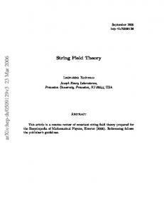
Figure 1: Action of the topological defect on a boundary field φab i can be described by enclosing it with an open defect attached to the boundary. The result is a collection ′ ′ (direct sum) of boundary fields φai b in all possible new boundary conditions allowed by fusion. The dots at the junctions represent simple normalization factors determined in subsection 4.2. For the sake of simplicity and concreteness we limit our discussion in this paper to topological defects of minimal models with diagonal partition function. These have been fully classified [58] and they are in one-to-one correspondence with primary operators. For these defects we find from the distributivity requirement (1.4), in a canonical normalization for boundary fields (3.23), that the X coefficients are given in terms of the normalized g-functions g ′ (2.22) and the normalized 6J-symbols (2.36) 1
′ ′ ′ ′ 4 dab Xia ′ b′ = (ga gb ga′ gb′ )
�
a, a′ , d b′ , b, i
�
.
(1.6)
For the special case of a = b this reduces, up to a normalization, to the result of Graham and Watts [60]. The action of the defect on boundary fields can be conveniently understood in terms of defects attached onto the boundary as in Figure 1. The defect endpoints can be freely moved along the boundary without changing correlators as long as the defect does not cross any operator insertion. The junction point can be viewed as an insertion of the identity operator (and not a traditional boundary condition changing operator) up to a normalization factor which we determine in subsection 4.2. Quite surprisingly however, the fusion rules of the open defect operators are twisted by an orthogonal similarity transformation when multiple boundary condition are generated by the defect. So instead of X Ndc e De DdDc = (1.7) e
which holds for the defect action on bulk states, the action on boundary operators obeys ! M −1 D d D c = Udc Ndc e De Udc . (1.8) e
5
Here U is a matrix, which for fixed c and d describes a discrete transformation in the space of multiplicity labels, which for fixed initial and final boundary conditions has its rows labeled by the intermediate boundary condition created by D c , and columns labeled by e the summation parameter of the direct sum on the right hand side. When we include also the initial and the final boundary conditions as part of the multiindices, i.e. {a, a′ , a′′ } and [e; a, a′′ ] respectively, the U matrix becomes orthogonal and it is surprisingly given by the Racah symbol (2.40) ′
(Udc ){a a
a′′ }[e; b, b′′ ]
= δab δa′′ b′′
�
c, a, a′ a′′ , d, e
�
.
(1.9)
From the explicit formula [10] for the boundary state in terms of the OSFT classical solution it follows that applying the defect operator to the open string field results in a boundary state encircled by the defect operator which gives a new consistent boundary state of the kind considered by Graham and Watts [60]. In formulas ||BDΨ ii = D||BΨ ii.
(1.10)
Therefore, assuming that a given solution ΨX→Y describes BCFTY in terms of BCFTX , upon action of the defect operator D, it will describe BCFTDY in terms of BCFTDX , i.e. DΨX→Y = ΨDX→DY . As a byproduct of our analysis we discover the interesting relation X daa (a′ ) i Xia Bj ga′ , Djd (a)Bji ga = ′ a′
(1.11)
(1.12)
a′ ∈d×a
relating bulk to boundary structure constants for different boundary conditions, where D is the coefficient of the defect operator (2.13) acting on a spinless bulk field (labeled by j). In order to be as self-contained as possible the paper includes some review material and it is organized as follows. In section 2 we review the basic definitions and properties of defects and defect networks in two dimensional CFT. We also introduce the duality matrices as generic solutions to the pentagon identity (which is a consequence of the topological structure of the networks and the basic fusion rules of the defects) and the related 6J and Racah symbols. In section 3 we review the basic construction of boundary states in diagonal minimal models and how topological defects act on them. In addition we review Runkel’s derivation of the boundary OPE coefficients and identify a particularly useful normalization for boundary fields. Section 4 is devoted to the main results of our work, namely the construction of open topological defect operators as maps between two boundary operator algebras which is compatible with the OPE. We present 6
two independent derivations of our results, one which is algebraic and which builds on the initial analysis by Graham and Watts [60] and one which is geometric and uses the properties of defect networks in presence of boundaries. Both our constructions clearly show that the composition of open topological defect operators follows the fusion rules only up to a similarity transformation whose precise structure is encoded in the Racah symbols. In section 5 we consider open topological defects as new operators in OSFT which map solutions to solutions. We show that the way OSFT observables are affected by the action of defects is consistent with the BCFT description and the interpretation of OSFT solutions as describing a new BCFT using the degrees of freedom of a reference BCFT. In section 6 we concretely present our constructions in the explicit example of the Ising model BCFT. Few appendices contain further results which are used in the main text.
2
Defects in conformal field theory
Consider two, generally distinct, 2d CFT’s glued along a one-dimensional interface. We assume that energy is conserved across this interface. Let (x0 , x1 ) be the coordinates of the system and the interface is placed at x1 = 0. From the conservation law ∂0 T 00 +∂1 T 10 = 0, we see that if T 10 is continuous then the total energy is conserved Z Z ∂ ∂ 1 00 dx T = dx1 1 T 10 = 0. (2.1) 0 ∂x ∂x Then we require that the momentum density T 01 = T 10 is continuous across the interface T 01 (x0 , x1 ) x1 →0+ = T 01 (x0 , x1 ) x1 →0− . (2.2)
Introducing the complex coordinates z = x0 + ix1 and z¯ = x0 − ix1 , the above condition is written as � � ¯ (¯ 0 1. 0 1 = lim T (z) − T¯ (¯ z ) (2.3) T (z) − T z ) lim z=x −ix z=x +ix 1 1 x →0
x →0
This condition also means that the system has invariance under conformal transformations which leave the shape of the defect line untouched, and the interface enjoying (2.3) is called a conformal interface or a conformal defect. The gluing condition (2.3) is usually implemented by giving a rule for how fields of these two CFTs are related at the interface, and conformal defects give a mapping from a field configuration of one theory to that of the other theory. The concept of conformal defects comes from the study of one dimensional impurity system [63, 64]. For a recent discussion of conformal defects see [65, 66, 67, 68]. 7
There are two special classes of conformal defects: the factorized defects and the topological defects. The factorized defects are purely reflective with respect to the energy flow, and the two CFTs do not communicate at all. This condition is given by requiring the energy current T 01 to be zero at the defect, or equivalently 0 1. 0 1, 0 1 = lim T¯ (¯ 0 1 = lim T¯ (¯ z ) z ) lim T (z) lim T (z) z¯=x −ix z=x +ix z ¯ =x −ix z=x +ix 1 1 1 1 x →0
x →0
x →0
x →0
x →0
x →0
x →0
x →0
(2.4) From (2.4) we see that the system is reduced to two separated BCFTs sharing the defect line as their common boundary. Also note that a conformal boundary can be viewed as an example of a factorized defect between a given bulk CFT and an empty c = 0 theory. On the other hand, topological defects are purely transmissive with respect to the energy, and this condition is expressed by the momentum conservation across the defect. From the conservation law ∂0 T 01 + ∂1 T 11 = 0, we see that if T 11 is continuous across the defect, the momentum is conserved. In complex coordinates, this condition is given by ¯ (¯ 0 1. 0 1 = lim T¯ (¯ 0 1 = lim T (z) 0 1 , z ) T z ) lim T (z) lim z¯=x −ix z¯=x +ix z=x +ix z=x −ix 1 1 1 1
(2.5) The energy momentum tensor does not see the defect, since its components are continuous across the defect line. Therefore, continuous deformations of topological defects do not change the value of correlation functions. A familiar example of a topological defect appears in the Ising model CFT, which is equivalent to the minimal model M(3, 4) with three primary fields {1, ε, σ}. In addition, there exists the disorder field µ which however is not mutually local with the spin field σ. The correlation functions containing both spin fields and disorder fields have branch cuts on their Riemann surface, and they are represented by disorder lines which connect a pair of disorder fields. Clearly the value of such correlation functions does not change by continuous deformations of disorder lines. In the above example, topological defects are curve segments with both end-points at disorder fields but we can consider more generic configurations in which defects join or end on a boundary, as we will review and discuss later.
2.1
Closed topological defects
A particularly class of defect operators are closed topological defects which are associated to homotopy classes of cycles on a punctured surface. The closed topological defects give rise naturally to closed string operators D which act on bulk fields by encircling them with the defect. Since both the holomorphic and antiholomorphic component of the energy momentum are continuous across the defect, the encircling defect loop can 8
be arbitrarily smoothly deformed and the defect action should also commute with the Virasoro generators ˜ n , D] = 0, [Ln , D] = [L ∀n. (2.6) By Schur’s lemma the action of the defect operator on the bulk states must be constant on every Verma module. Then we can concentrate on the action of D on the bulk primary operator φ(i,¯i,α,α) ¯), where i and ¯i are labels for the Virasoro representation of the ¯ (z, z holomorphic and antiholomorphic part and α and α ¯ are corresponding multiplicity labels. Let a be a label classifying the topological defects then, following Petkova and Zuber [58], we can write a D a φ(i,¯i,α,α) ¯) = D(i, ¯), (2.7) ¯i,α,α) ¯ (z, z ¯ (z, z ¯ φ(i,¯i,α,α) a with constant coefficients D(i, . This can be written by ¯i,α,α) ¯
Da =
X
¯
a (i,i,α,α) ¯ D(i, , ¯i,α,α) ¯ P
(2.8)
(i,¯i,α,α) ¯ ¯ ¯ where P (i,i,α,α) is the projector on the Verma module labeled by (i, ¯i, α, α ¯ ). a To determine the coefficients D(i,¯i,α,α) , let us consider the modular transformation of ¯ the torus partition function with a pair of closed topological defect lines. There are two ways for evaluating this. One way is to consider time slices parallel to the defect line, obtaining the following expression � � c c ¯ Za|b =Tr (D a )† D b q˜L0 − 24 q¯˜L0 − 24 X (2.9) a ∗ b = (D(j, q)χ¯j (q¯˜). ¯ j,α,α) ¯ ) D(j,¯ j,α,α) ¯ χj (˜ (j,¯ j,α,α) ¯
The other way is to consider time evolution along the defect line. Let Vi¯i;x y denotes the multiplicity of the Virasoro representation (i¯i) appearing in the spectrum in this time slicing ¯ ¯i , (2.10) Ha|b = Vi¯i;a b Ri ⊗ R then the partition function is written as X q ). Za|b = Vj¯j;a b χj (q)χ¯j (¯
(2.11)
(j,¯ j,α,α) ¯
From modular invariance of the Virasoro characters, we can connect (2.9) and (2.11), and obtain a bootstrap equation �∗ � X b a D , (2.12) Sji S¯j¯i D(i, Vi¯i;a b = ¯ ¯i,α,α) (i,i,α,α) ¯ ¯ j¯ j
9
which in paticular states that the rhs should be a positive integer. For the diagonal minimal models there is a simple solution to (2.12) Dia =
Sai , S1i
Vi¯i;a b =
X
Nai k Nk¯i b .
(2.13)
k
We can check this result with the help of the Verlinde formula [69] Nijk =
X Sil Sjl S ∗
kl
S1l
l
.
(2.14)
On the right hand side of the first equation of (2.13), index a runs over the irreducible representations of the Virasoro algebra, and from this expression, we see that there are as many distinct topological defects as primary operators. Plugging back to (2.8), we obtain that X Sai P i. (2.15) Da = S1i i
It then follows that these operators obey the fusion algebra X Da Db = Nabc Dc ,
just like the conformal families of the primary fields X [φa ] × [φb ] = Nabc [φc ].
(2.16)
(2.17)
c
This follows by a simple computation ! ! X Sai Sbi X Sbj XX X Sai Sci i Pi Pj = Pi = Nabc P , S S S S S 1i 1j 1i 1i 1i i j i c i
(2.18)
where in the last equality we used Verlinde formula (2.14).
2.2
Defect networks
To get a more conceptual understanding of topological defects, it is useful to consider networks of topological defects, where the defects are allowed to join in trivalent vertices. Let us state now some minimalistic assumptions: defects can be decomposed into elementary ones. The labels of the elementary defects define naturally an associative algebra. For two elementary defects a and b we define the product of labels a × b as a free sum of labels of the elementary defects which arise upon fusing defect a with defect b. The associativity follows from the topological nature of defects. 10
a a
a
b
b
b non-elementary =
p c
topological
=
defect
d c
c
d
d
Figure 2: The topological nature of defects implies that an“s-channel” configuration with an elementary defect should be equivalent to a “t-channel” configuration with a composite, but still topological defect. a a
b
b =
p
Fpq
a b c d
q
q
c
d c
d
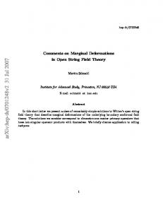
Figure 3: Elementary defect network move. Another important assumption is that there is always an identity defect, labeled as 1 or 1, which can be freely drawn or attached anywhere without changing anything.2 The most powerful property of topological defects, is that they can be freely deformed, without changing the value of any correlator, as long as they do not cross the position of any operator insertion or another defect. Therefore, a small piece of defect network in the“s-channel”-like configuration, shown on the left hand side of Figure 2, composed of four defects joined by an intermediate one, can be deformed into an alternate “tchannel”-like configuration where the new defect will in general no longer be elementary one. Decomposing it into a linear combination of elementary defects, defines a set of � � a b a priori unconstrained coefficients Fpq c d , see Figure 3. In many circumstances these coefficients are known, but in order to be self-contained and perhaps more general, let us ignore this knowledge and proceed by following the consequences of consistency. 2
At this point our conventions differ from some of the literature on the subject e.g. [70].
11
The most important consistency condition comes from considering the defect network shown in Figure 4. By following the fusion rule in Figure 3 from one starting to one a b
c
d
s q a b
c
d
a b
e Fps
p
b c a q
Fqt
c
d
s
s d a e
q
t e
Fqr pc de a b
c
p
e
Fsr cb dt d
r
a b Fpt
c
b r a e
d r
t
e
e
Figure 4: Pentagon identity as a consistency condition for fusion of defects. final configuration along two different paths depicted by arrows in Figure 4, one finds the celebrated pentagon identity3 X � � � � � � � � � � Fps ab qc Fqt as de Fsr cb dt = Fqr pc de Fpt ab re . (2.19) s
By the MacLane coherence theorem, this equation is enough to guarantee the consistency of the fusion rule in Figure 3 for any possible defect network. This is not to say that other identities are not of interest, but that those required for consistency are implied by the pentagon identity. 3
This identity differs from the one given in� [72]� by transposition of columns in every F . For unoriented � �
defects this difference is immaterial as Fpq
a b c d
= Fpq
b a d c
. For oriented defects one has to specify
carefully an orientation. Our implicit orientation (always downwards in Figure 4) is the same as in [73] and others [74], but differs from the one required to match the formulas of Moore and Seiberg [72, 71].
12
A simple property of the F following from our definition and the natural normalization for the trivial identity defect is that Fpq
�
a b c d
�
=1
whenever 1 ∈ {a, b, c, d}.
(2.20)
Using this in the pentagon identity by setting e = 1 (which requires also q = d, a = t and p = r) one finds the orthogonality relation X � � � � Fps ab dc Fsr cb da = δpr . (2.21) s
For p 6= r the left hand side of (2.19) still makes sense, but the right hand side would contain fusion matrix elements with non-admissible label, so the only consistent value for the left hand side is zero. Alternatively, one can of course apply the elementary move again to the right hand side of Figure 3 viewed sideways. Let us now consider defect networks containing closed loops. An arbitrary such network can be reduced via the elementary move in Figure 3 to a network without any closed loops. The simplest defect network with a loop is of course a single loop, but let us start with a slightly more general configuration shown in Figure 5 of a bubble with two external defect lines attached. As long as there are no operators put inside the bubble, it can a i
j
=
1
i
b
a
a
a j
F1k aa bb
= k
b
i
j
k b
b
⇓ a i
j b
=
δij F1i
a b a b
i
i
Figure 5: Defect bubble network. When no operators are present inside, the topological bubble can be shrank to zero size, yielding a numerical factor symmetric under the exchange of a and b labels. shrink leaving behind a pure number. This already tells, that the two external lines must carry the same label otherwise, upon shrinking, one would expect a defect changing operator insertion. These operators carry nontrivial conformal weight and thus the correlator scaling properties would contradict those expected for a network of topological defects. 13
Attaching an auxiliary line of identity defect (see Figure 5) allows us to find a simple expression for the bubble in terms of the �F -matrix. In rotation invariant theories for � a b unoriented defects the numerical factor F1i a b must be symmetric in a and b, as follows by considering the 180◦ degree rotation. As a corollary we find that a bubble with no defects attached, which is the same thing as if two identity defects were attached, is equivalent to an overall factor ga′ =
1 F11
� �, a a a a
(2.22)
which we identify with the normalized g-function of the defect.4 Another corollary is an expression for the sunset diagram in Figure 6. Since it can be a c b
1
= F11
a a a a
F1a
b c b c
= θ(a,b,c)
Figure 6: Defect sunset network gives rise to an S3 symmetric factor θ(a, b, c). viewed as a symmetric bubble on a loop in two possible ways, it follows that θ(a, b, c) = θ(a, c, b) = θ(c, b, a),
(2.23)
and hence it enjoys the full S3 permutation symmetry. Analogously, we can introduce ˜ b, c) = θ(a,
1
� � � �, F11 aa aa Fa1 cb cb
(2.24)
which, as a consequence of pentagon identity (setting t = q = 1 together with s = e = d = a, r = b and p = c in (2.19)) satisfies ˜ b, c), ga′ gb′ gc′ = θ(a, b, c)θ(a,
(2.25)
˜ b, c) also possess the S3 permutation symmetry. and hence θ(a, Another peculiar identity which can be obtained by the sequence of moves in Figure 7 is , where S is the modular S-matrix. It is In the context of the minimal models this is equal to SS1a 11 thus the value of the g-function of the boundary condition associated to the defect via the folding trick, normalized by the g-function of the trivial defect. In non-unitary theories (e.g. for the Lee-Yang model) or theories with oriented defects this quantity may coincide with the usual normalized g-function only up to a sign. 4
14
a
b
a =
1
b
F1c aa bb
c
c =
c∈a×b
c∈a×b
⇓ 1 F11
a a a a
1
× F11
Nabc
=
b b b b
c
1 F11
c c c c
Figure 7: Derivation of the Verlinde-like formula. In the second step we use the S3 symmetry of the bubble factor θ(a, b, c). 1
1
� � � � F11 aa aa F11 bb bb
=
X c
Nabc
1 F11
�
c c c c
�.
(2.26)
It might come as a surprise that this equation is a consequence of the polynomial pentagon identity (2.19). To see that it is indeed the case, one may proceed in two steps. Starting with the orthogonality relation (2.21), setting p = r = 1, adjusting accordingly the other indices, and using the relation (2.25) one derives easily (2.26). For the minimal models, the relation (2.26) is in fact nothing but the Verlinde formula for the first row (or column) of the S-matrix S1a S1b X = Nabc S1c . S11 c
(2.27)
thanks to the relation between the modular S-matrix and the F -matrices (which follows from the formulas in [71], see also e.g. (E.9) in [83]) X Sij 1 � = e2πi(hi +hj −hk ) S11 F11 k
k k k
k∈i×j
�,
(2.28)
� � ��−1 S1j which for i = 1 simplifies to gj′ = S11 = F11 jj jj . The next natural step is to consider a defect loop with three external defect lines attached, as in Figure 8. Applying the elementary defect network move to any pair of vertices connected by an internal defect line, we find the elementary vertex with a bubble on one of the external lines, and as before we can replace the bubble by the corresponding factor. In general this would yield a Z3 symmetric expression which follows directly from the pentagon identity (2.19) by setting t = 1 which requires also s = d, r = b and e = a with the help of (2.25). For unoriented parity-invariant defects in parity invariant CFT’s the symmetry is enhanced to S3 . 15
k
k
a
b
=
Fck
j i a b
× F1k
a b a b
−1
c i
j
i
j
Figure 8: Triangular defect network. When no operators are present inside, the topological triangle can be shrank to zero size, yielding a numerical factor with S3 permutation symmetry under the exchange of (i, a), (j, b) and (k, c) labels. The symmetries of the F matrices are actually much larger and can be nicely manifested by considering a defect network in the shape of tetrahedron, see Figure 9. It can be drawn as such on a Riemann sphere, but the resulting identities should have universal validity. Let us now choose any triangular face, e.g. (abc), and shrink it to a point picking i c
j
b k
a
Figure 9: Tetrahedral defect network. When no operators are present inside the faces, the topological tetrahedron can be shrank to zero size, yielding a numerical factor with S4 permutation symmetry under the exchange of the faces with (a, b, c), (a, j, k), (b, k, i) and (c, i, j) labels. up the triangle factor as in Figure 8. This results in the sunset diagram, see Figure 6, which we have already evaluated. Combining the factors, one quickly arrives at � i, j, k TET a, b, c
�
≡ =
�
j a � � � F1k aa bb F1k ii
Fck
� i b � � � j k k F 11 j k k �
1 θ(a, b, k)θ(i, j, k)Fck gk′
� j i . a b
(2.29)
The notation is such that the labels in the upper row always form an admissible triplet, i.e. i ∈ j × k. We could have chosen an arbitrary face of the tetrahedron for reducing the triangle and due to the Z3 cyclicity of the defect triangle in Figure 8, we would have obtained one out of three possible expressions. Altogether we get 12 different expressions which must 16
be equal to each other, and which correspond to the orientation preserving subgroup A4 of the tetrahedral group S4 . The Z3 subgroup cyclically permutes the columns � i, j, k TET a, b, c
�
=
� j, k, i TET b, c, a
�
=
� � k, i, j TET , c, a, b
(2.30)
while the Z2 × Z2 subgroup is switching upper and lower labels simultaneously in two different columns � i, j, k TET a, b, c
�
=
� i, b, c TET a, j, k
�
=
�
� a, b, k TET i, j, c
=
�
� a, j, c TET . i, b, k
(2.31)
The equality of the three expressions (2.30) follows already from the pentagon identity, but (2.31) does not. The reason is that in deriving (2.31) we have assumed that all defects were unoriented. For oriented defects some labels in the identity (2.31) must be replaced by the conjugate labels to account for the change of orientation. In the special case of parity invariant defects in parity invariant theories the tetrahedral defect network is invariant under the full tetrahedral group S4 which in addition to the generators of A4 contains also 12 transformations combining rotations with a single reflection. The additional identities can be generated with the help of � i, j, k TET a, b, c
�
=
�
� j, i, k TET . b, a, c
(2.32)
These are the symmetries of the classical or quantum Wigner’s 6J symbol. This object however differs from the 6J symbol by a tetrahedral invariant normalization factor (see discussion in section 2.2.2), and resembles thus an object often called T ET in the literature, see e.g. [76] or [75]. Another difference would arise in the case of oriented defect, where the tetrahedral invariance of the defect network would be broken.5 2.2.1
Specular symmetries
As follows from the definition of the F -matrix, see Figure 3, invariance under 180◦ rotation for unoriented defects implies � � � � Fpq ac db = Fpq db ac . (2.33) Similarly parity invariance of both the theory and the defect (with respect to any axis) implies a stronger condition Fpq
� � a b c d
= Fpq
�
c d a b
5
�
= Fpq
�
b a d c
�
.
(2.34)
Also because of the fact, that up to the normalization factor, this object obeys the pentagon identity without signs, it is more reminiscent of the classical Racah W-coefficient.
17
Of course, the two identities (2.34) together imply (2.33). All these identities are true in the Virasoro minimal models. Mathematically, the symmetry of the F matrix (2.33) is equivalent to the condition (2.31) under the assumption of the pentagon identity, or in particular (2.30). Analogously, � � �TET � k TET under the same assumption, the symmetries (2.34) are equivalent to a,i, b,j, kc = b,j, a, i, c and
� i, j, k TET a, b, c
�
2.2.2
=
� j, i, k TET b, a, c
�
respectively.
6J symbols, Racah symbols and their identities �
�TET
From the defect network manipulations we have seen that a,i, b,j, kc obeys the same tetrahedral symmetries as classical or quantum Wigner symbol. Such an object is by no means unique, since a product over the four tetrahedron vertices of an S3 invariant function of the three corresponding edges will always have the tetrahedral symmetry. A particularly useful combination is what we call the normalized 6J symbol �
i, j, k a, b, c
�
1
= p
θ(i, j, k)θ(i, b, c)θ(a, j, c)θ(a, b, k) s 1 θ(a, b, k)θ(i, j, k) �j i � Fck a b , = ′ gk θ(i, b, c)θ(a, j, c)
�
� i, j, k TET a, b, c
(2.35)
(2.36)
which enjoys also the full tetrahedral symmetry for unoriented defects. If it were not for the prefactor 1/gk′ it would have obeyed the pentagon identity, since Fpq
� � a b c d
→
Λ(a, b, q)Λ(c, q, d) �a Fpq c Λ(c, a, p)Λ(p, b, d)
b d
�
,
(2.37)
is an exact symmetry of the pentagon identity (2.19) for an arbitrary function Λ(i, j, k) of an admissible triplet6 . Due to cyclicity of θ, one can arrange their arguments, so that the full prefactor under the square root in (2.36) can be viewed as a gauge transformation. Hence the 6J symbol obeys the following pentagon-like identity X � �� �� � � �� � c, b, s d, s, t d, c, r d, c, r r, b, t gs′ a, = . (2.38) q, p a, e, q b, t, s p, e, q a, e, p s
When one of the entries equals 1, the 6J symbol simplifies �
� i, c, b 1, b, c
6
1 =p ′ . gb gc′
(2.39)
Further discussion of this “gauge symmetry” observed by Moore and Seiberg [71] is relegated to appendix A.
18
This offers a very promising procedure to solve the polynomial equations in the general P case. Given the fusion rules, we first solve the much simpler system ga′ gb′ = c Nabc gc′ . This system of equations in rational CFT’s has as many solutions as we have labels. Every solution corresponds to a single column of the modular S-matrix normalized by its first element. Then we can solve the pentagon identities (2.38) by imposing the symmetries on the 6J symbol. We have checked that for Lee-Yang model, Ising model and tricritical Ising model these over-determined polynomial systems have a unique solution. A fundamental property of the 6J symbol is gauge invariance under the symmetry (2.37) which holds for any Λ which is S3 -invariant and subject to the additional condition Λ(1, a, a) = 1. Another very useful object which will play an important role in the following sections of this paper is what we call Racah symbol following the terminology of Coquearaux7 � � � � p i, j, k ′ ′ i, j, k g g (2.40) ≡ k c a, b, c . a, b, c It obeys the full pentagon identity, X� �� c, b, s a, q, p
d, s, t a, e, q
s
��
d, c, r b, t, s
�
=
�
d, c, r p, e, q
��
� r, b, t , a, e, p
(2.41)
and can be therefore identified with the F matrix in a given special gauge �
� c, b, s a, q, p
Rac = Fps
�
b c a q
�
.
(2.42)
A peculiarity of this gauge is that � � F1iRac aa bb
� � Fi1Rac ab ab
=
=
s
gi′ . ga′ gb′
(2.43)
When one of the entries of the first two columns equal 1, the Racah symbol simplifies � i, c, b 1, b, c
�
= 1.
(2.44)
This object, like the 6J symbol, is also invariant under the gauge transformation (2.37). Just like a generic solution to the pentagon identity, the Racah symbols obey the orthogonality condition X� �� � b, a, q c, a, s = δps . (2.45) c, d, p b, d, q q
7
What Coquearaux [76] calls geometrical Racah symbols, or Carter et al [75] call the 6j symbol are our F matrices.
19
When we manipulate defect networks we don’t have necessarily to fix a gauge for the involved F matrices. This has to be contrasted with the F matrices arising from the transformations of the conformal blocks which are uniquely determined once the conformal blocks are normalized, by giving the coefficient of their leading term. It would be interesting to know whether there is a specific normalization choice which also fixes the gauge for the defect networks. This may involve a careful study of defect changing fields, which goes beyond the scope of this paper.
3
Boundaries in conformal field theory
Conformal boundary conditions in 2D CFT’s have to satisfy a number of consistency conditions spelled out explicitly in [77, 78]. This section is a review of some of these consistency conditions in diagonal minimal models and of the action of topological defects on the fundamental boundary states.
3.1
Boundary conditions in minimal models
From the bulk perspective, conformal boundary conditions in 2D CFT’s are encoded in the conformal boundary states which are required to obey a number of necessary conditions. The most elementary requirement of preserving the conformal symmetry forbids the twodimensional energy and momentum to flow through the boundary, which leads to the gluing condition � ¯ −n ||Bii = 0. Ln − L (3.1) The set of linearly independent solutions was written down by Ishibashi [79]. The Ishibashi states are in one-to-one correspondence with spinless bulk primaries V α X ¯ −J |Vα i |Vα ii = M IJ (hα )L−I L (3.2) IJ
=
X n
|n, αi ⊗ |n, αi
i h 1 ¯ −1 + · · · |Vα i. L−1 L = 1+ 2hα
(3.3) (3.4)
The multi-indices I, J, with I = {i1 , ..., in } appearing in the first line label the nondegenerate descendants in the conformal family of Vα , and M IJ (hα ) is the inverse of the Gram matrix hV α |LI L−J |Vα i. We denoted LI = Li1 Li2 . . . Lin and L−I = L−in L−in−1 . . . L−i1 . The Ishibashi state (see the second line) is as a sum over a basis of states (which are orthonormal wrt the Gram matrix) in the Verma module over the chiral part of the primary Vα . 20
A highly non-trivial consistency requirement is given by Cardy’s condition. Consider the partition function on a finite cylinder with two boundary conditions a and b. Viewed in the “closed string” channel, the diagram can be interpreted as a matrix element between two boundary states ||aii and ||bii. In the “open string” channel it becomes a trace over the Hilbert space of the CFT with the two boundary conditions a and b
where
1 c � c ¯ hha||˜ q 2 (L0 +L0 − 12 ) ||bii = TrHopen q L0 − 24 , ab
q = e2πiτ ,
q˜ = e−2πi/τ ,
(3.5)
(3.6)
and τ = R/L is given by the radius and length of the cylinder. It is well known that for minimal models with diagonal partition function Cardy’s condition is solved by a set of fundamental boundary states, explicitly given by [80] ||Bi ii =
X Sj q i |jii, j S1j
(3.7)
where Sij are the entries of the modular matrix and i and j denote the Virasoro representation which are present in the minimal model. Therefore in this case there is a one-to-one correspondence between chiral primaries and fundamental boundary conditions. The most general boundary condition consistent with Cardy’s condition is obtained by taking positive integer linear combinations of the above fundamental boundary states, in the case of diagonal minimal models.
3.2
Runkel’s solution for boundary structure constants
Boundary operators generally change the boundary conditions. The multiplicity of a boundary operator in the Virasoro representation k, changing the boundary conditions from i to j is the integer coefficient Nijk appearing in the fusion rules of the theory φi × φj =
X
Nij k φk .
(3.8)
k
While one could extract the spectrum of boundary operators from the cylinder amplitude between two boundary states, to compute their OPE structure constants one has to resort to the 4-pt conformal bootstrap. To this end, let us consider a 4pt boundary function
� (abcd) bc cd da Gijkl (ξ) ≡ I ◦ φab (3.9) i (0)φj (1)φk (ξ)φl (0) UHP , 21
where I(z) = − 1z . We can compute it in two ways using different OPE channels
� (abcd) bc cd da Gijkl (ξ) = I ◦ φab i (0)φj (1)φk (ξ)φl (0)
� ab bc cd = h ◦ φda l (0)h ◦ I ◦ φi (0)h ◦ φj (1)h ◦ φk (ξ)
� ab bc cd = ξ hi +hj −hl −hk I ◦ φda l (0) φi (1) φj (1 − ξ) φk (0) (dabc)
= ξ hi +hj −hl −hk Glijk (1 − ξ),
(3.10)
where h(z) = z−ξ . We now express the four point functions in terms of the structure z constants and the four point conformal blocks X (abc) p (cda) p (abcd) Gijkl (ξ) = Cij Ckl G(aca) (3.11) pp F (i, j, k, l; p)(ξ), p
where the conformal blocks are given by the formula X F (i, j, k, l; p)(ξ) = βI (hi , hj , hp )βJ (hk , hl , hp )GIJ (hp )ξ hp +|J|−hk −hl ,
(3.12)
I,J
where I is a Virasoro multiindex, GIJ is the matrix of inner products in a highest weight representation of Virasoro algebra, and the β coefficients are defined via X (abc) p βI (hi , hj , hk ) bc L φac (y). (3.13) φab (x)φ (y) = Cij i j hi +hj −hk −|I| −I p (x − y) p,I Notice that F do not depend on any normalization of boundary operators. The conformal blocks in ξ can be linearly related to the the conformal blocks in 1 − ξ via precisely chosen F matrices X � � blocks l i F (k, l, i, j; p)(ξ) = Fpq F (i, l, k, j; q)(1 − ξ). (3.14) k j q
Then, using (3.11) and (3.14), we find from (3.10) X � (dab) p (bcd) p (dbd) blocks l Cli Cjk Gpp = Fqp k
i j
q
(abc) q
�
Cij
(cda) q
Ckl
G(aca) qq ,
(3.15)
where the two point functions are given in terms of the three point functions as (aca) 1 G(aca) = Cpp ga . pp
(3.16)
This can be further simplified to8 (abd) l
Cip
(bcd) p
Cjk
=
X
blocks Fqp
q
8
(cda) q
Use Ckl
(aca) 1
Cqq
(acd) l
= Cqk
(ada) 1
Cll
(aba) 1
and Cii
�
l i k j
�
(bab) 1
ga = Cii
22
(abc) q
Cij
gb .
(acd) l
Cqk
.
(3.17)
Runkel [82] has observed9 that this equation can be exactly solved by setting (abc) k
Cij
blocks = Fbk
�
a c i j
�
,
(3.18)
thanks to the pentagon identity. We can find a more convenient expression for the structure constants by �changing the � blocks a b normalization of the boundary operators. To this end, let us express Fpq in terms c d of the normalized 6J symbols s � � θ(b, d, p)θ(c, a, p) �b, a, q � blocks a b ′ Fpq = g . (3.19) q c d θ(c, d, q)θ(b, a, q) c, d, p Runkel’s solution then becomes (abc) k
Cij
= =
� � blocks a c Fbk i j
s
gk′ gb′
s
= gk′
s
θ(c, j, b)θ(i, a, b) �c, a, k� θ(i, j, k)θ(c, a, k) i, j, b
θ(c, j, b)θ(i, a, b) �c, a, k� θ(i, j, k)θ(c, a, k) i, j, b
v u θ(c,j,b) θ(i,a,b) u √g ′ g ′ g ′ √ ′ ′ ′ u c j b gi ga gb = t θ(i,j,k) θ(c,a,k) √′ ′ ′√′ ′ ′ gi gj gk
gc ga gk
�
c, a, k i, j, b
�
.
(3.20) (3.21)
(3.22)
From here we see that there is a special choice of normalization of the boundary fields, in which10 sp gi′ gj′ gk′ �c, a, k� (abc) k Cˆij = . (3.23) θ(i, j, k) i, j, b The Racah symbol is gauge invariant, but the object θ(i, j, k) has to be computed from � � blocks a b Fpq , i.e. c d gi′ � �. θ(i, j, k) = (3.24) F1iblocks jj kk 9
Generalizations have been studied in [83, 84, 85]. This expression for the boundary structure constants is particularly √ ′ ′ ′interesting since the square of gi gj gk bulk in a canonical normalization the prefactor coincides with the bulk structure constants, Cijk = θ(i,j,k) for bulk operators where the coefficient of the two point functions are set universally to one times the sphere partition function. 10
23
3.3
Defect action on boundary states
As we have seen in section 2.1, defects act naturally on bulk operators by encircling them. Cardy boundary states are (non-normalizable) states in the space of bulk operators ||Ba ii =
X Sai √ |iii, S1i i
so, analogously, the action of the defect operator is given by [60] X Da ||Bb ii = Nabc ||Bc ii,
(3.25)
(3.26)
c
as follows by a computation almost identical to section 2.1, using again Verlinde formula and the fact that the projectors obey P i |jii = δji |jii. Now we can easily offer an alternative proof for the observation of [11] that OSFT P β makes predictions for the coefficients of the boundary states ||BX ii = β BX |βii β BX BYβ
BRβ
=
X
NXYZ BZβ ,
(3.27)
Z
under the assumption that the reference D-brane ||Rii allowed an OSFT solution describing ||X ii and that such a solution could have been re-interpreted on a D-brane ||Y ii sharing the relevant Verma modules as ||Rii. Assuming that the defect operator acts as a multiple of the identity on each Verma module and that as an operator it is selfconjugate (or possibly antiselfconjugate) under BPZ conjugation then the coefficients of the boundary states satisfy hV β |D||Rii hV β |D||X ii = , hV β ||Rii hV β ||X ii and hence
β BDR
BRβ
=
β BDX β BX
,
(3.28)
(3.29)
where DR and DX stands for D-branes obtained by fusing defect D onto R or X branes. The new DX brane itself is either fundamental or should be an integer linear combination of such and therefore β β X BX BDR β = B = NDXZ BZβ , (3.30) DX β BR Z
which matches the formula (3.27) derived from OSFT by reinterpreting a solution ΨR→X on the DR brane. It is one of the goals of this paper to explain this coincidence. 24
4
Attaching defects to boundaries
In this section we define and study the action of topological defects on boundary fields. This was partially done by Graham and Watts [60] for boundary operators which do not change the boundary conditions. We will generalize their algebraic approach to the full open string spectrum, including the important case of boundary condition changing operators. In addition we will provide an independent geometric derivation using defect networks. We determine how an open string defect acts as an operator mapping the boundary operator algebra of a system of boundary conditions to a closed subset of the operator algebra of a new system of boundary conditions. Then we study the composition of such operators and we show how is this related to the fusion rules of the theory. We first proceed in a completely algebraic way, imposing the condition that the OPE must commute with the action of an open topological defect. This is a non-trivial constraint that can be solved for the coefficients defining the open string defect (see later) and, together with an appropriate twist-invariance condition, allows to uniquely determine such coefficients, thanks to the pentagon identity. Then we show that the composition of open topological defects is governed by the fusion rules of the theory but, differently from the closed string case, there is a non trivial rotation in the Chan-Paton’s labels corresponding to coincident final boundary conditions. This rotation is in fact a similarity transformation. In the second subsection we show that our algebraic results can be independently obtained in a purely geometric way by manipulating the involved defect networks with boundary. Our goal is to define an action of defects on the open string Hilbert space D : Hopen → Hopen .
(4.1)
This general action is further specified by decomposing Hopen into fundamental boundary conditions M H(ab) , (4.2) Hopen = a,b
where, when a 6= b, the corresponding states are boundary condition changing fields. Let d be a label for a topological defect, then the open string topological defect is a linear map M ′ ′ H(a b ) . (4.3) D d : H(ab) → a′ ∈ d × a b′ ∈ d × b
This map is injective but in general is not surjective (the defect maps from a given open string Hilbert space, onto a “bigger” one). This is how open strings feel the fact that a 25
topological defect, in general, maps a single D-brane into a system of multiple D-branes, according to the fusion rules of the underlining bulk CFT. As in the bulk case, Schur’s ′ ′ lemma implies that the operator D restricted to H(a,b) → H(a ,b ) should be a multiple of the identity on every Verma module Viri in H(a,b) . Assuming that all states can be obtained by acting Virasoro operators on primary states, which is true in unitary CFT’s, the open string defect action is fully specified by X a′ b′ dab Xia , (4.4) D d φab = ′ b′ φi i a′ ∈ d × a b′ ∈ d × b
where the φ’s are the boundary primary fields, allowed by the involved boundary conditions.
4.1
Algebraic construction
In this subsection we will determine the above-defined X-coefficient in an algebraic way. Then we will inspect how the composition of open topological defects is related to the fusion of defects in the bulk and to the fusion rules of the theory. 4.1.1
Defect coefficients from OPE
A simple consistency condition for the action of open-string defects has been introduced by Graham and Watts [60] � � d bc � bc d ab D d φab D φj (y) . i (x)φj (y) = D φi (x)
(4.5)
Using the general ansatz (4.4) as well as the operator product expansion, the constraint (4.5) takes the explicit form X (a′ b′ c′ )k (abc)k dbc dab dac (4.6) = Cij Xka Xka ′ b′ Xkb′ c′ , ′ c′ Cij b′ ∈d×b
(abc)k
where Cij are the boundary structure constants. Restricting ourselves to the An series of the minimal models, see section 3.2, the boundary structure constants can be written as s p ab bc gi′ gj′ gk′ �c, a, k� ni nj (abc)k , (4.7) Cij = nac θ(i, j, k)blocks i, j, b k ab where nab i are generic normalizations of boundary fields with the convention that ni = 1 for the canonical normalization (3.23). With this explicit form of the structure constants
26
it immediately follows that (4.6) admits a general solution dab Xia ′ b′ =
� ′ � N(d, a, a′ ) nab i b , i, a , ′ ′ ′ nai b d, a , b N(d, b, b′ )
(4.8)
thanks to the pentagon identity (2.41). The pentagon identity doesn’t fix the constants N(d, c, c′ ), but their are in fact fixed by imposing the parity condition11 dba dab Xia ′ b′ = Xib′ a′ ,
(4.9)
which, using the properties of the Racah symbol in section 2.2.2, gives �2 s ′ ′ � N(d, a, a′ ) ga′ gb , = ′ N(d, b, b ) ga′ gb′ ′ so that we can take N(x, y, z) =
q�
x, x, 1 z, z, y
�
=
The X coefficients take the explicit form dab = Xia ′ b′
=
� � nab i Rac a b F ′ ′ ′ ′ di a b nai b
q
�
gy′ gx′ gz′
.
� � � � a d Rac b d F ′ 1b a d b d � � Rac a b F1i a b
Rac F1a ′
1 nab i ′ ′ ′ ′ 4 (g g g ′ gb′ ) ′ ′ a b a nai b
� 41
�
� a, a′ , d . ′ b , b, i
(4.10)
(4.11)
(4.12) (4.13)
Notice that, differently from the boundary structure constants, the defect coefficients X don’t depend on the crossing symmetry properties of the conformal blocks, since only the Racah symbols are involved in their definitions. 4.1.2
Fusion of open string defects
Let us now consider the fusion of topological defects on general boundary fields. To this end, we need to calculate the subsequent action of D c and D d on φab i . As we saw in (4.4), after the first action of D c there are multiple boundary conditions in general, and it is natural to arrange the r.h.s. of (4.4) into a matrix regarding a′ and b′ as matrix indices. 11
In this work we consider only 2D CFT’s which are separately invariant under C, P and T discrete symmetries. The parity symmetry P is related to the twist symmetry in the corresponding SFT [86].
27
That is
a′1
.. D c φab = i . a′m
...
b′1
a′ b′1
cab 1 Xia ′ b′ φi 1 1 .. .
b′n a′ b′n
...
cab 1 Xia ′ b′ φi 1 n .. .
...
cab m Xia ′ b′ φi m n
...
a′ b′1
m cab Xia ′ b′ φi m 1
a′ b′n
,
(4.14)
where a′i ∈ c × a and b′j ∈ c × b. The number of labels a′i is given by the number of nonzero Nca i s, and the number of labels b′j is that of Ncb j s. The right hand side is a m × n matrix, and m and n are given by X X ′ ′ m= Nca ai , n= Ncb bj , (4.15) i
j
′ ′
′ ′
ab cab a b respectively. We also write this equivalently as (D c φab = Xia . Similarly, after ′ b′ φi i ) d the subsequent action of D , we have
...
b′1
Ma′1 b′1 . .. D d D c φab i = .. . a′1
a′m
Ma′m b′1
... ... ...
M
a′p b′q
...
b′′ 1 da′ b′
a′′ b′′
p q cab 1 1 Xia ′ b′ X ′′ ′′ φi ia1 b1 p q � � a′p b′q cab .. = ... ≡ D d Xia ′ b′ φi . p q da′p b′q a′′ b′′ cab a′′ Xia′p b′q Xia′′s b′′ φi s 1 s
a′′ 1
Ma′1 b′n .. , .
(4.16)
Ma′m b′n
where the submatrix Ma′p b′q is given by
b′n
1
... ... ...
b′′ t da′ b′
a′′ b′′ t
p q cab 1 Xia ′ b′ X ′′ ′′ φi ia1 bt p q .. .
da′ b′
a′′ b′′ t
p q s cab Xia ′ b′ X ′′ ′′ φi ias b p q t
This is a s × t matrix, and s and t are given by X X ′′ ′′ t= Ndb′q bj , s= Ndap ′ ai , and the size of the matrix D d D c φab i is given by ! X X X ′ ′′ s × t = Nda′ ai Nca ap × p
b′q ∈c×b
. (4.17) (4.18)
j
i
a′p ∈c×a
i, p
28
X j, q
b′′ j db′q
N
Ncb
b′q
!
.
(4.19)
From (4.16) and (4.17) we see that to identify the position of components in (D d D c φab i ), ′ ′ we need to refer to both the intermediate boundary condition (a b ) and the final boundary condition (a′′ b′′ ). We then introduce a composite label {a a′ a′′ } and express the above result as �{a a′ a′′ }{b b′ b′′ } � d c ab �a′ b′ �a′′ b′′ da′ b′ a′′ b′′ cab . (4.20) = Xia D d D c φi ≡ D D φi ′ b′ Xia′′ b′′ φi
P For the defect action on the bulk space we have D d D c = e Ndce D e . For the action on the boundary operators we have to replace the ordinary sum by a direct sum, since different defects map to different Hilbert spaces fe M 1 M �a′′ b′′ .. D e φab = (4.21) , . i e∈d×c fe M k
where
e ab a′′ b′′ e ab a′′ b′′ Xiaj′′ b′′ φi 1 1 . . . Xiaj′′ b′′ φi 1 h 1 h 1 1. .. . fe ≡ D ej φab . M = . . . . . i j ′′ ′′ ′′ ′′ ej ab ag bh ej ab ag b1 . . . Xia′′g b′′ φi Xia′′g b′′ φi
(4.22)
h
1
′′
Now we introduce the labels [e; a, a ] to represent M
e∈d×c
D e φi
![e; a, a′′ ][f ; b, b′′ ]
≡ D e φab i
�a′′ b′′
′′ b′′
eab a δef = Xia ′′ b′′ φi
δef .
(4.23)
Clearly the two expressions (4.20) and (4.23) are different, but notice that they have the same dimensions thanks to the identity X X Nij k Nkl m = Nim k Nkl j . (4.24) k
k
� P �P a′ a′′ ′d That is, as explained in (4.19), the number of the labels {a a′ a′′ } is given by a′′ N N , ′ ac a a �P � P e a′′ while the number of the labels [e; a, a′′ ] is given by a′′ . These two nume Ncd Nae bers are equal, as explained e.g. in [71]. Similarly, we also conclude that the number of the labels {b b′ b′′ } and that of the labels [e; b, b′′ ] are the same. This suggests that there might be a similarity transformation linking the two matrices, D d D c φi
�{a a′ a′′ }{b b′ b′′ }
"
= Udc
M
e∈d×c
29
!
−1 D e φi Udc
#{a a′ a′′ }{b b′ , b′′ }
,
(4.25)
where Udc is a real invertible matrix with matrix indices {a a′ a′′ } and [e; a ˜, a˜′′ ]. Sub� L e stituting (4.20) for (D d D c φi ) and (4.23) for e∈d×c D φi , this equation is expressed as X X {a a′ a′′ }[e; a˜ a˜′′ ] ′ ′′ ˜′′ −1 [f ; ˜ da′ b′ e˜ a˜b cab δ ef (Udc ) b, b ]{b b b } . (4.26) Xia Udc Xi˜ ′′ b′′ Xia′ b′ = a′′˜b′′ [e; a ˜a ˜′′ ] [f ; ˜b, ˜ b′′ ]
dab Since Xia ′ b′ is the Racah symbol with some extra factors (4.8), the equation (4.26) is again reminiscent of the pentagon identity (2.41). In fact, we find that the following Udc is a solution N(c, a, a′ )N(d, a′ , a′′ ) ( c, a, a′ ) (a = a ˜) and (a′′ = a˜′′ ), M(d, e, c)N(e, a, a′′ ) a′′ , d, e {a a′ a′′ }[e; a ˜, a ˜′′ ] (Udc ) = (4.27) 0 (a 6= a ˜) or (a′′ 6= a ˜′′ ),
where the factor N(x, y, z) is the same as that appearing in (4.8), and M(x, y, z) is a −1 nonzero arbitrary real number. To check (4.26), notice that the inverse matrix Udc is given by M(d, e, c)N(e, a, a′′ ) �a′′ , a, e � −1 [e; a, a′′ ]{a a′ a′′ } (Udc ) = (4.28) ′ , N(c, a, a′ )N(d, a′ , a′′ ) c, d, a
as can be checked from the orthogonality relation (2.45). A natural choice for M(x, y, z) is � ′ � 41 q � � gy Rac z z , (4.29) M(x, y, z) = N(x, y, z) = Fy1 x x = gz′ gx′
which makes Udc an orthogonal matrix ′
(Udc ){a a
a′′ }[e; a ˜, a ˜′′ ]
′′ ]{a a′
−1 [e; a = (Udc ) ˜, a˜
a′′ }
.
(4.30)
This can be easily checked by substituting (4.29) into (4.27) and (4.28), obtaining ′
(Udc ){a a
a′′ }[e; a, a′′ ]
=
�
c, a, a′ a′′ , d, e
�
,
(4.31)
and, using the tetrahedral symmetry of the Racah symbol ′′ ]{a a′
−1 [e; a, a (Udc )
a′′ }
=
� � ′′ a , a, e ′ c, d, a
=
�
c, a, a′ a′′ , d, e
�
′
= (Udc ){a a
a′′ }[e; a, a′′ ]
.
(4.32)
A comment on the appearance of the matrix structures in the above discussion. We have arranged the elements of the matrices in a particular way as in (4.16), (4.17) and (4.21) for illustrative purpose, but we don’t have to necessarily adhere to this ordering of rows and columns. Indeed, from (4.27) we see that the mixing only occurs when
30
(a, b) = (˜a, ˜b) and (a′′ , b′′ ) = (˜a′′ , ˜b′′ ), and with a suitable ordering of the columns and the rows we can bring Udc into a block-diagonal form. The net mixing is therefore given by X � � � � cab da′ b′ ef eab Ua′ e ad′′ ca Xia Xia Ub′ f bd′′ cb , (4.33) ′′ b′′ Xia′ b′ = ′′ b′′ δ e, f
where Ua′ e
�
� d c ′′ a a
{a a′ a′′ }[e; a a′′ ]
= Udc
=
�
c, d, e a′′ , a, a′
�
.
(4.34)
In section 4, we will explicitly work out this block-diagonalization in the example of the Ising model CFT.
4.2
Geometric construction
Imagine a disk correlator with a number of bulk operator insertions. Placing a topological defect parallel to the boundary and sufficiently close to it, so that there are no bulk operators between the defect and the boundary, one can smoothly deform the defect so that it fuses onto the boundary without affecting any correlator. From the bulk perspective, as we reviewed in Section 2, these correlators can be viewed as overlaps of the new boundary state D||Bii with the vacuum excited by the vertex operators. Already by considering disk amplitudes without operator insertions, we find a number of interesting relations, illustrated in Figure 10 X X gb′ � � , (4.35) gb = F11 dd dd gb′ = gd′ ′ ′ b ∈d×b
b ∈d×b
from which it follows (assuming the existence of the identity boundary condition) that the normalized g function of the defect is in fact the g function of the corresponding boundary condition, normalized by the g-function of the identity boundary condition gd′ ≡
1 �
� F11 dd dd
gd , g1
=
(4.36)
or, considering the “sunset” disk diagrams gb � ′� F1b dd bb′
=
gb′ F1b′
�
�, d b d b
(4.37)
whose actual numerical value depends on the chosen gauge for the F matrices. We remind that consistency of defect network manipulations only imply that the involved F matrices obey the pentagon identity and therefore the gauge for the F matrices used for defect manipulations is not fixed. This has to be constrasted with the F blocks matrices entering 31
b
d
S11 S1d
=
b
b
b S11 = S1d b ∈d×b
b
d = F1b
b
b
1
1
=
d b d b
F1b
d b d b
Figure 10: Defects can be used to derive a relation between the g-functions of different boundary conditions. Defect attached to the boundary can be shrank in two different directions, producing consistent answer thanks to the identities for the fusion matrix F . the boundary structure constants which, as we have reviewed in section 3.2, imply a very specific gauge choice once the conformal blocks are canonically normalized. Now, what happens by attaching a defect to a boundary, when there are boundary operators present? The conformal weight of such operators cannot change, so they must become new boundary operators in the same Virasoro representation, but interpolating between the new boundary conditions, and possibly modified by a new normalization constant. To understand what happens to the boundary operators it is convenient to proceed in steps. First, imagine to partially� fuse a defect d on a boundary segment b . Such a fusion � d b brings in a nontrivial factor F1b′ d b , see Figure 11.
d
d =
1
F1b
d
d b d b
b ∈d×b
b
b
b
b
Figure 11: Partial fusing of a defect onto a boundary. This factor can be assigned to the left and right junctions between the defect, the original boundary and the new boundary and it is natural to distribute it evenly between the two junctions. This implies that when a d defect fuses on a boundary a to give a superposition of boundary conditions a′ = d × a, the involved junction must be accomq � � panied by a factor of F1a′ dd aa . This factor will be represented by a boldface dot at the 32
d d =
a
X
a′ ∈d×a
r
F1a′
h
d a d a
i
a
d =
a
X
a
a
a′ ∈d×a
Figure 12: A defect fusing onto a boundary. Every produced fundamental boundary condition is accompanied by a junction factor which is graphically represented as a thick dot.
d d Dd φab = i
= a
φi
b
F1a a ∈d×a b ∈d×b
d a d a
a
a φi b
b
F1b
d b d b
d = a ∈d×a b ∈d×b
a
a φi b
b
Figure 13: The geometric description of a defect action on a boundary field. Notice the √ F factors at the junctions. junction, see Figure 12. The action of a defect on an open string state is explicitly defined in Figure 13 Once the above geometrical defintion is given, defect distributivity � � d bc � bc d ab D φj (y) , (4.38) D d φab i (x)φj (y) = D φi (x)
follows rather naturally. Since the defect can be partially fused onto the boundary as in Figure 14 (using the rule in Figure 11), the only issue one has to take care of is the � � d b ′ normalization factor F1b d b which is accounted by the non-trivial normalization of the junctions. 4.2.1
Defect action on a boundary field from network manipulations
It remains to compute the explicit X coefficients of the defect action X X dab a′ b′ D d φab Xia . ′ b′ φi i = a′ ∈d×a b′ ∈d×b
33
(4.39)
d
d
1 a
a φi
b
φj
c
c
=
F1b
d b d b
a
b ∈d×b
d
a φi b
b
b
d = b ∈d×b
a
c
d
a φi b �
φj c
b
b
φj c
c
�
Figure 14: Defect distributivity. In the second line the factor F1b′ dd bb has been absorbed into the two c-number insertions at the junction points denoted by thick dots. In order to make use of the needed defect network manipulations, we uplift the boundary conditions and the boundary insertions into a defect network with a line carrying the i representation and ending on a chiral defect-ending field, placed at the boundary with identity boundary conditions. This is explained in detail in appendix B. In our setting this move is essentially equivalent to a corresponding three-dimensional manipulation in the topological field theory description of defects in RCFT [57], see in particular [70], but it has its own two-dimensional description given in B. After this topological move, the defect coefficient X can be easily computed as in Figure 15. The α coefficients explicitly depend on the chosen normalization for boundary fields (with the convention that nab i =1 for the canonical choice (3.23) )and on the chosen gauge for defect networks, see (B.7), giving in total � � s a b q q ab F ′ ′ � � � � ′ ′ di γ(i, a , b ) ni a b dab d a d b � � ′ ′ F F = Xia ′ b′ 1a 1b ′ ′ d a d b γ(i, a, b) nai b F1i a b a b
q � nab i Rac d F = ′ ′ ′ 1a d nai b =
a a
�
�
Rac a b � Fdi a′ b′ � � F1iRac aa bb
1 nab i (ga′ gb′ ga′ ′ gb′ ′ ) 4 a′ b′ ni
�
b′ , a′ , i a, b, d
�
.
q � Rac d F1b ′ d
b b
�
(4.40)
Notice in particular that the gauge dependent factors in the α’s (B.7) conspire together with the gauge dependence of the defect manipulation in Figure 15 to give an overall gauge invariant result which only depends on the normalization choice for the boundary fields, as it should: acting a defect on a boundary field doesn’t depend on the defect’s gauge. 34
d d a ab Dd φab i
=
a
a φi b
αiab
=
b
a
b φi
1
b 1
d
= αiab
F1a
a
d a d a
a
=
αab = ai b αi
F1a
d a d a
F1a
Fdi
d a d a
F1i
a b a b
b
F1b
d b d b
a
F1i aa bb dab Xia b
F1b
b
i 1
a b a b
d b d b
1
F1b
a b a b
Fdi
b
φi
1
αiab
i
φi
1
d b d b
a
φi
b
φai b
dab Figure 15: Defect network manipulations determining the defect coefficients Xia ′ b′ . Notice that the boundary insertion i is traded for a defect ending on the boundary. Along such a defect an ab-bubble is collapsed, after F -crossing on the original defect line d. The two junctions at which the d defect joins the boundary corresponds to square roots of F matrix elements.
35
4.2.2
Defect fusion from network manipulations
Let us now see how we can use similar manipulations to reduce the composition of two defects c and, subsequently, d to a direct sum of defects e, in the fusion of c and d. We start with a general boundary field Φ and act the defects on it XXX X �
DdDcΦ =
a,b
X
=
i
a′ ,b′ a′′ ,b′′
X
{a,a′ ,a′′ } {b,b′ ,b′′ }
D d D c φab i
�a′ b′ �a′′ b′′
�{a,a′ ,a′′ },{b,b′ ,b′′ } DdDcΦ .
(4.41)
Then we can perform the manipulations shown in Figure 16
d c { a, a , a Dd Dc φab i
} { b, b , b
}
= a
a
a φi b
b
b
d =
d a d a
F1a
c a c a
F1a
Fa e
e
d c a a
e∈c×d
c a φi b
a
Fb e
c d b b
F1b
c b c b
F1b
d b d b
b
e d a d a
F1a
= e∈c×d
F1e
d c d c
c a c a
F1a F1a
e a e a
Fa e ad ac
Fb e cb bd a φi b
a
b
F1b
c b c b
F1b
d b d b
F1e
d c d c
F1b
e b e b
[e;aa ][e;bb ]
{ aa a
(Udc )
} [e;aa ]
D
f
(ab) φi
T Udc
[e;bb ]{ bb b
}
f ∈d×c
Figure 16: Defect network manipulations determining the fusion rules of open string defects.
′ ′′ }[e;a,a′′ ]
(Udc ){aa a
v � � � � u u F1a′′ d a′′ F1a′ c a � u c a d a � � � � Fa′ e d′′ =t a F1a′′ ee aa F1e dd cc 36
c a
�
=
�
c, d, e a′′ , a, a′
�
,
(4.42)
which coincides with (4.31) Notice that in the geometric approach there naturally appears the transpose of the U matrix on the right ! M T D d D c Φ = Udc D e Φ Udc . (4.43) e∈d×c
Before closing this section, let us comment on one particularly surprising aspect of the relation (4.43). It is a bit reminiscent of some sort of generalized non-abelian projective P e representation12 of the closed string defect algebra D d D c = e∈d×c D and one may ask whether the corresponding 2-cocycle condition is satisfied. This is equivalent to the condition of associativity of the defect algebra on the open string fields � � De Dd Dc = De Dd Dc . (4.44) To prove associativity, following the steps in Figure 17, one has to show that X X � � � � � � � � � � � � � Ua′ g ad′′ ac Ub′ g cb bd′′ Ua′′ h ae′′′ Ua′′ f ae′′′ ad′ Ub′′ f bd′ be′′′ Ua′ h af′′′ ac Ub′ h cb bf′′′ = g
f
g a
�
Ub′′ h
�
g e b b′′′
(4.45) To see that, let us start by writing the pentagon identity for the Racah symbols (2.41) in a more convenient form X� � �� � �� �� � p, e, r r, e, p c, b, s d, s, t d, t, s = . (4.46) d, c, q a, b, t a, q, p a, e, q b, c, r s
Using this identity we can express the product of the two factors on the left hand side depending on the a-type labels (any of the labels a, a′ , a′′ and a′′′ ) Ua′′ f
�
e d a′′′ a′
�
Ua′ h
�
� f c ′′′ a a
= =
�� � � � ′ ′′′ �� f, a′′′ , a′ a ,a , f c, f, h d, e, f = ′′ ′′′ ′ ′′′ ′ ′′ a, c, h e, d, a a , a, a a ,a ,a X� �� �� � e, h, g e, g, h d, c, g . c, d, f a, a′′′ , a′′ a, a′′ , a′ g
�
(4.47)
This last expression upon multiplication by the remaining b-type terms from the left hand side of (4.45) can now easily by summed over label f using the relation (4.46) and one ends up precisely with the right hand side of (4.45). This concludes the proof of associativity.
5
Topological defects in open string field theory
In this section we would like to study how topological defects act on OSFT solutions. As we have already stated, OSFT provides a new way to explore the possible conformal 12
Instead of the usual representation on vectors up to a phase, this behaves as a representation on matrices up to a similarity transformation.
37
�
.
e
d De Dd Dc φab i
{ a, a , a } { b, b , b }
c
= a
a
Ua
e d f a a
Ub
a φi b
a
b
b
d e f b b
b
Ua g
d c a a
Ub g
c d b b
e
f g
c a
a φi b
a
Ua h
f a
c a
Ub h
b
b
a
a
c f b b
Ua
a φi
b
e g h a a
Ub
b
b
g e h b b
h
a
a
φi
b
b
Figure 17: Proof of associativity. Fusing together three defects attached to a boundary in two different ways results in a consistency condition (4.45) for the U matrix. The resulting condition follows from the pentagon identity for the Racah symbol (2.41). boundary conditions of a bulk CFT, by solving the equations of motion. Let us then briefly review how can we use OSFT to analyze BCFT’s with central charge c different from 26 [10, 11]. The open string star algebra is factorized in the Hilbert space of the c = −26 ghosts’ BCFT, with standard boundary conditions, and in the matter c = 26 38
BCFT, whose boundary conditions can be generic. In our application of OSFT to BCFT we will further assume that the matter BCFT is the tensor product of a BCFTc (whose properties we wish to study) times a compensating “spectator” BCFT26−c BCFTtotal = BCFTc ⊗ BCFT26−c ⊗ BCFTghost .
(5.1)
In the total corresponding star algebra we restrict to the subalgebra where only descendants of the identity in the spectator sector are excited. Then we can search for classical solutions with the most general ansatz at ghost number one X X X i(ab) gh R Ψ= aIJK Lc−I |φab (5.2) i i ⊗ L−J |0i ⊗ L−K c1 |0i, i
a,b
I,J,K
where Lc−I = L−in L−in−1 · · · L−i1 for 0 ≤ i1 ≤ i2 ≤ · · · in , and J, K are defined in the same way. The label i runs over all Virasoro representations of BCFTc that are allowed by the pair of boundary conditions a, b (with, possibly, non-trivial multiplicities). In the case of diagonal minimal models we have that i ∈ a × b. If some fundamental boundary condition i(ab) appears multiple times (trivial multiplicities), then the coefficients aIJK are matrices in the degeneracy labels (Chan-Paton factors). A possible approach to search for new boundary conditions in the CFTc factor (5.1) is to solve the OSFT equation of motion with the ansatz (5.2). In particular the boundary state corresponding to these new boundary conditions can be computed from OSFT gauge invariant observables [10]. In the previous section we have defined the action of topological defects on generic boundary operators including those which change the boundary conditions. This then naturally defines an action of a topological defect on open string fields X X X i(ab) � gh R DdΨ = aIJK Lc−I D d |φab (5.3) i i ⊗ L−J |0i ⊗ L−K c1 |0i, a,b
i
I,J,K
because [Lmatter , D] = 0. n
(5.4)
It follows that, noticing that [bn , D] = 0 and [cn , D] = 0, [Q, D] = 0.
(5.5)
It is also not difficult to establish that D d (φ ∗ χ) = (D d φ) ∗ (D d χ)
∀φ, χ.
(5.6)
Indeed, assuming the BFCT of interest to us is unitary and therefore its total Hilbert space is spanned by the direct sum of the Verma modules over the primaries, this condition just 39
follows from the compatibility with the OPE (4.5) and the conservation laws of the star product [13, 14, 15]. Concretely, given two descendants string fields L−I φab i (0)|0i and bc L−J φj (0)|0i, we can express their star product schematically as bc L−I φab i (0)|0i ∗ L−J φj (0)|0i =
X K
P
VIJ K (hi , hj )L−K e
vk L−k
bc φab i (x)φj (y)|0i,
(5.7)
where the coefficients VIJ K , vk as well as the insertion points x and y are explicitly known or calculable. Acting with D d , one can bring it through all the Virasoro generators, use formula (4.5) and use again formula (5.7) to reassemble the left hand side. Therefore open topological defects map solutions to solutions in OSFT QΨ + Ψ ∗ Ψ = 0
→
Q(DΨ) + (DΨ) ∗ (DΨ) = 0.
(5.8)
The main issue is now the physical interpretation of these new solutions.
5.1
Defect action on string field theory solutions
In this subsection we will derive the following key result: given a solution ΨX→Y which shifts the open string background from BCFTX to BCFTY , we will show that the solution DΨX→Y shifts from BCFTDX to BCFTDY , where the subscript denotes the boundary conditions obtained by fusing the defect D on the X and Y boundary conditions respectively. In formulas DΨX→Y = ΨDX→DY . (5.9) To do so we will evaluate the OSFT observables of DΨX→Y and show that they fully agree with the observables of the r.h.s of (5.9). In particular we will show that the boundary state of DΨX→Y is just the result of the defect action on the boundary state of ΨX→Y ||BDΨ ii = D||BΨ ii.
(5.10)
Notice that in OSFT there appears a natural interplay between the open string defect operator D and its closed string counterpart D. 5.1.1
Computation of S [DΨ]
Before studying the full boundary state, it is instructive to look at the simpler case of the OSFT action. Carrying out the summation on I, J and K in (5.2) we can write the string field as XX Ψ= Ψab (5.11) i , a,b
40
i
where the label i and ab denote the Virasoro representation and boundary conditions of BCFTc . In order to treat both the quadratic and cubic terms in the action (1.1) at the same time, it is useful to prove the more general statement Tr[(D d Ψ1 ) ∗ · · · ∗ (D d Ψn )] =
gd Tr[Ψ1 ∗ · · · ∗ Ψn ], g1
(5.12)
where Tr is the usual Witten integral, combined with trace over Chan-Paton factors. By defect distributivity (D d Ψ1 ) ∗ · · · ∗ (D d Ψn ) = D d (Ψ1 ∗ · · · ∗ Ψn ), it is enough to show that Tr[D d Ψ] =
gd Tr[Ψ]. g1
(5.14)
Using the results of previous sub-sections the l.h.s. can be easily evaluated as X X X {a,a′ },{a,a′ } daa ] Tr[D d Ψ] = Xia ′ a′ Tr[Ψi a
=
i
XX a
i
a′ ∈d×a
δi1
X
(5.13)
{a,a′ },{a,a′ }
Tr[Ψ1
],
(5.15)
a′ ∈d×a
since only the boundary Virasoro representation i = 1 can contribute to the Witten daa integral. Moreover, on general grounds, X1a ′ a′ = 1 since a defect always maps the identity to the identity, as can be easily checked in the explicit example (4.8). To continue we simply notice that ga′ {a,a′ },{a,a′ } Tr[Ψaa (5.16) Tr[Ψ1 ]= 1 ], ga since the two traces involve the same operator algebra and only differ in the normalization (a) of the vacuum amplitudes ga ≡ h 1 idisk , and similarly for a′ . We therefore have ! X X ga′ d aa . (5.17) Tr[D Ψ] = Tr[Ψ1 ] ga ′ a a ∈d×a
Using the Pasquier algebra for the g-functions, see equation (2.26) and (4.36) X gd ga , ga′ = g1 ′
(5.18)
a ∈d×a
concludes the proof of (5.12). In the next section we will see an alternative geometric approach making use of defectnetwork manipulations, Figure 19. 41
What we derived holds at the level of the Witten integral therefore, remembering that the defect trivially commutes with the BRST charge, it is immediate to see that for any open string field Ψ we have gd SOSFT [Ψ]. g1
SOSFT [D d Ψ] =
(5.19)
Suppose now we have a solution ΨX→Y which describes BCFTY as a state in BCFTX . This means in particular we have a solution whose action is given by SOSFT [ΨX→Y ] =
1 (g − gY ) . 2π 2 X
It follows that the defect-acted solution will have an action given by � � gd 1 gd gX gd gY d SOSFT [D ΨX→Y ] = SOSFT [ΨX→Y ] = 2 . − g1 2π g1 g1
(5.20)
(5.21)
The difference entering into the above equation is nothing but the difference in the identity-coefficients (g-functions) of the two boundary states obtained by acting the closed string defect D d on the source and target boundary states ||BX ii, ||BY ii, connected by the solution ΨX→Y gd gX |1ii + · · · g1 gd gY D d ||BY ii = D d (gY |1ii + · · · ) = |1ii + · · · . g1
D d ||BX ii = D d (gX |1ii + · · · ) =
(5.22) (5.23)
This is the first non-trivial check that (5.9) indeed holds. 5.1.2
Computation of the Ellwood invariant
Let us now see how the Ellwood invariant is affected by the defect action. To start with, it is useful to derive an identity involving the bulk-boundary structure constants (a)Bji , the g-functions and the open and closed defect coefficients. The required identity is obtained by computing a disk amplitude with a spinless bulk field V j (z, z¯), a boundary field φaa i (x) and a defect loop d encircling the bulk field. See Figure 18. The correlator can be computed by acting the closed string defect on the closed string field V j , or by partially attaching the defect to the boundary, producing an open string defect acting on the boundary field φi (x). Calling, in generality, Did the defect coefficient, P i.e. D = i Did Pi , where Pi projects in the i-th Verma module in the bulk, we get the identity X daa (a′ ) i (5.24) Djd (a)Bji ga = Xia Bj ga′ , ′ a′ a′ ∈d×a
42
b Djd
V
j
d φi
b φi
Vj
=
d =
b
b
Vj
φi
b ∈d×b
b
b V
=
j
b φi
d
b ∈d×b
Xibdbbb
=
V
j
φi
b ∈d×b
Figure 18: Two equivalent ways of computing a bulk-boundary correlator in presence of a closed string defect d. which in the case of diagonal minimal models reads13 Sdj S1j
(a)
Bji ga =
X
Rac Faa ′
a′ ∈d×a
�
� a d (a′ ) i Bj ′ i a
ga′ .
(5.25)
Thanks to this relation it is easy to algebraically show that X X X {a,a′ },{a,a′ } daa ] Xia TrV j [D d Ψ] = ′ a′ TrV j [Ψi a
i
a′ ∈d×a
X X X
′ � (a )B i � j Rac a d Faa′ i a′ (a) i B j a′ ∈d×a
ga′ {a,a′ },{a,a′ } TrV j [Ψi ] g a a i X X Sdj X X = TrV j [Ψaa TrDd V j [Ψaa i ] = i ] S 1j a a,α i∈a×a i =
= TrDd V j [Ψ],
(5.26)
where in the second line we have used that the two involved open/closed couplings (carrying the same Virasoro labels but different boundary conditions) only differ by the overall 13
Boundary fields are here canonically normalized (3.23). In the special case where the boundary field S carries the identity representation it coincides with (4.42) of [83]. In this case we have (a)Bj1 ga = √ aj S1j
and analogously for the new boundary conditions a′ , and so the relation reduces to the Verlinde formula X Sdj Saj = S a′ j . S1j ′ a ∈d×a
43
a
a
Tr V Dd Ψ =
d a
a ∈d×a
d
a f (1) ◦ Ψaa =
F1a
V
a
d a d a
a ∈d×a
f (1) ◦ Ψaa
V
a
a
d = a,p a ∈d×a p∈d×d
F1a dd aa
Fa p ad da
p
V
d f
(1)
◦Ψ
aa
= a
V
f (1) ◦ Ψaa
= Tr Dd V [Ψ]
Figure 19: Defect networks manipulations for the Ellwood invariant of a defect-acted open string-field. The dashed line corresponds to the identification of the �2 left and right part of the open string, via the identity conformal map f (1) (z) = 1+iz . Notice that thanks 1−iz to the junctions normalizations and the consequent F -matrix orthogonality relation, only the identity defect p = 1 stretches between the boundary and the defect d, making d a genuine closed string defect. When V = 1 this also gives a geometric proof of (5.14). bulk-boundary structure-constant B and the g-functions, due to the identical operator algebra involved in their calculation. Again, this can be shown geometrically manipulating defect networks, as shown in Figure 19, and the result is correctly independent on the gauge used for defect manipulations. 5.1.3
KMS and KOZ boundary state
Having obtained in generality how an Ellwood invariant is affected by the action of an open string defect, let us see how the OSFT boundary state constructed in [10] (KMS from now on) behaves under the defect action. The KMS approach gives a simple recipe to directly compute the coefficients of the matter Ishibashi states of the boundary state associated to a given solution Ψ in terms of a minimal generalization of the Ellwood invariant. In the setting of this paper, where we are assuming that the matter BCFT is the tensor product of a diagonal rational BCFT of central charge c and a “spectator” sector of central charge (26 − c), the required generalization of the Ellwood invariant is simply achieved by assuming that the spectator sector contains a free boson (call it Y ) with Dirichlet boundary conditions, see [11, 10] for further details. Then the KMS 44
construction is usefully summarized as ||BΨ iiKMS = njΨ
X j
njΨ |V j ii
!(c)
⊗ ||B0 ii(26−c) ⊗ ||B0 iighost
= (2πi) TrV˜ j [Ψ − Ψtv ] √ 2 V˜ j (z, z¯) = c¯ c V j e2i 1−hj Y (z, z¯).
(5.27) (5.28) (5.29)
Since we have shown that TrV [DΨ] = TrDV [Ψ] for any string field, the KMS construction applied to the solution DΨ will obviously give14 ||BDΨ iiKMS = D||BΨ iiKMS .
(5.30)
At last let’s also consider the other available construction of the boundary state in OSFT, given by Kiermaier, Okawa and Zwiebach (KOZ) [21]. KOZ geometrically construct a BRST-invariant ghost number three closed string state obeying the level matching − b− 0 = L0 = 0. This closed string state is conjectured to be BRST equivalent to the BCFT boundary state and in fact the two coincide for many known analytic solutions. The main ingredient of this construction is a choice of half-propagator strip in the background of a classical solution Ψ, whose left edge and right edge are glued together, to form an annulus-like surface, which is used to build the closed string state � Z s � I π2 ¯ (L + L ) KOZ Pexp − dt [LR (t) + {BR (t), Ψ}] . (5.31) ||BΨ ii =es 0 0 s
0
The various objects entering the above definition are defined in [21], but for us it is sufficient to recall that the quantity Pexp[...] represents a half-propagator strip of lenght H s, in the background of the classical solution Ψ, and that the symbol s identifies the initial left edge of the strip with the final right edge. The internal boundary of this annulus-like surface (corresponding to the propagation of the open string midpoint) defines a closed string state, the KOZ boundary state. If, instead of the original classical solution Ψ on BCFTX we replace the defect-acted solution DΨ on BCFTDX , then by defect distributivity on the star product (and the obvious commutativity with the b-ghost insertions) we will recover a closed string defect extending along the midpoint line, which is nothing but a closed-string defect operator acting on the original KOZ boundary state, see Figure 20 � Z s � I π2 ¯ (L + L ) KOZ Pexp − dt [LR (t) + {BR (t), DΨ}] ||BDΨ ii = es 0 0 s
14
= D||BΨ ii
KOZ
0
.
(5.32)
A simple consequence of this is that acting with a topological defect on a tachyon vacuum solution, the new solution solution will still be the tachyon vacuum (the boundary state will still vanish), although expressed with the degrees of freedom of the new BCFT D(X).
45
d×X
(1)
BR , Ψ
d
n=0
=
d ×
d
(1)
X BR , Ψ
d closed string patch
∞
X
∼
BR , Ψ
d×
BDΨ
d closed string patch
∞ KOZ
BR , Ψ
(2)
n=0
X
X
X BR , Ψ
= D BΨ
(n)
BR , Ψ
(n)
KOZ
Figure 20: Pictorial representation of the KOZ boundary state for a defect-acted solution (the boundary integrals in the “Pexp” operation, as well as other details, are not shown, as they are not important for our argument). Thanks to the defect distributivity, the various open string defects result in a single defect-loop encircling the closed string coordinate patch.
6
Ising OSFT example
In this section we would like to illustrate our general findings on the concrete example of open string field theory for the Ising model [11]. This is the simplest unitary diagonal minimal model and has c = 21 . It has three irreducible Virasoro representations, denoted as 1, ε and σ with well-known fusion rules ε×ε = 1
ε×σ = σ
(6.1)
σ × σ = 1 + ε. The bulk fields are all spinless and also labeled by 1, ε and σ. There are three possible fundamental boundary conditions also denoted as 1, ε and σ which describe the fixed (±) and free boundary conditions for the spins in the underlying lattice model. We will refer to the conformal boundary conditions of the Ising model as the Ising “D-branes”.
46
(2)
6.1
Defect action on Ising boundary fields
In the Ising model there are three (fundamental) topological defects. They can act on bulk field via closed-string defect operators, with the following composition rules Dε2 = D1
(6.2)
Dσ D ε = Dε Dσ = Dσ Dσ2
(6.3)
= D1 + Dε ,
(6.4)
which realize the fusion rules (6.1). Now we would like to construct the open string defect operators and study their composition rules according to section 4. The general boundary field on a system of N1 1-branes, Nε ε-branes, and Nσ σ-branes has the form (11)
L 1 (ε1) Ψ = ε P¯ε 1
¯ (σ1) Q σ
σ
ε
1
σ
(1ε)
Qσ
(1σ)
(εε)
Rσ
Pε
M1 ¯ σ(σε) R
(εσ)
(σσ) N1
+
(σσ) Nε
,
(6.5)
where the (a, b) component is a Na ×Nb matrix with respect to the Chan-Paton indices. We have chosen this presentation since topological defect operators are blind to Chan-Paton factors. The upper indices inside the parenthesis represent the left and the right boundary conditions, which are also indicated outside the matrix for later convenience,and the lower index is the Virasoro label. Each entry of (6.5) is a generic matrix-valued state in the Verma module indicated by the corresponding subscript, and allowed by the boundary conditions. This expression can also represent an open string field of the form (5.2, 5.11). As a useful example, let us study the fusion of two σ defect operators, Dσ2 , on the boundary field (or open string field) (6.5). From (4.4) and the concrete value of the defect coefficients X for the Ising model BCFT (see appendix C), applying the Dσ on the open string field (6.5) results in a matrix with a larger size
{1σ}
Dσ Ψ =
{1σ} (σσ)
L1
1 ¯ (σσ) {εσ} √ P ε 2 1 ¯ (1σ) {σ1} 1/4 Q σ 2 {σε}
1 ¯ (εσ) Q 23/4 σ
{εσ} (σσ) √1 Pε 2 (σσ) M1 (1σ)
¯σ 21/4 R 1 ¯ (εσ) − 1/4 Rσ 2
47
{σ1} 1
{σε}
(σ1)
Q 23/4 σ
(σ1)
1 − 21/4 Rσ √ (1ε) 2Nε
Q 21/4 σ
21/4 Rσ
(11)
N1 √ (ε1) 2Nε
(σε)
1
(σε)
(εε)
N1
.
(6.6)
Here indices {ab} (a, b = 1, ε, σ) outside the matrix keep track of changes of the left and the right boundary conditions; for example, the (1,1) component of the matrix has the indices {1σ}{1σ}, and the boundary condition of the corresponding entry has been changed as (σσ) (11) Dσ : L1 7→ L1 . (6.7) the (1,2) component of the matrix has the indices {1σ}{εσ}, and correspondingly, σ1ε (σσ) Dσ : Pε(1ε) 7→ Xεσσ Pε ,
(6.8)
σ1ε where Xεσσ = √12 , and so on. Note that the action of Dσ increases the number of branes in general, because it changes the σ-brane into a 1-brane and an ε-brane. Now the system has Nσ 1-branes, Nσ ε-branes and (N1 + Nε ) σ-branes. Applying Dσ again we obtain
{1σ1}
{1σ1} (11)
L1
0 {εσ1} 0 Dσ2 Ψ = (ε1) ¯ {εσε} P ε 1 (σ1) ¯ {σ1σ} √ Q 2 σ ¯ (σ1) √1 Q {σεσ} 2 σ {1σε}
{1σε}
{εσ1}
0
0
(εε)
{εσε} (1ε)
Pε
(ε1)
0
M1
(11)
0
0
0
M1
1 ¯ (σε) Q 2 σ ¯ (σε) − 12 Q σ
¯ σ(σ1) R
L1 (1ε) P¯ε
Pε
(εε)
(σ1)
¯σ −R
¯ (σε) √1 R 2 σ ¯ (σε) √1 R 2 σ
{σ1σ}
{σεσ}
(1σ) √1 Qσ 2 1 (εσ) Q 2 σ (1σ) Rσ (εσ) √1 Rσ 2 (σσ) N1
(1σ) √1 Qσ 2 (εσ) − 12 Qσ (1σ) −Rσ (εσ) √1 Rσ 2 (σσ) Nε
(σσ)
(σσ)
Nε
N1
which has an equal number of rows and columns given by 2(N1 + Nε + Nσ ). On the other hand, (D1 ⊕ Dε ) Ψ is given by
[1;11]
[1;εε]
[1;σσ]
[ε;1ε]
[ε;ε1]
[ε;σσ]
(1ε) Pε (εε) M1 ¯ σ(σε) R
(1σ) Qσ (εσ) Rσ (σσ) (σσ) N1 + Nε
0
0
0
0
0
0
0
0
0
0
0
0
0
0
0
0
0
0
(11) [1;11] L1 (ε1) ¯ [1;εε] Pε ¯ (σ1) [1;σσ] Qσ
[ε;1ε] [ε;ε1] [ε;σσ]
(εε)
L1
(1ε) P¯ε ¯ (σε) √1 Q σ 2
(ε1)
Pε
(11)
M1 √ (σ1) ¯σ 2R
(εσ) √1 Qσ 2 √ (1σ) 2Rσ (σσ) (σσ) N1 − Nε
,
(6.9)
.
(6.10)
This is clearly not equal to (6.9). While the closed defect operators Dd obey the defect algebra (6.4) which is strictly isomorphic to the Verlinde fusion algebra, this is not the case for the open string defect operators Dd . As discussed in section 4, we need to take 48
into account the similarity transformation (4.31) and (4.32) in order to connect (6.10) with (6.9). In this case, the similarity transformation is given by
{1σ1}
Uσσ
{εσ1} = {εσε} {σ1σ} {1σε}
{σεσ}
{1σ1}
{εσ1} = {εσε} {σ1σ}
[1;1,1]
[1;ε,ε]
[1;σ,σ]
[ε;1,ε]
[ε;ε,1]
[ε;σ,σ]
1
0
0
0
0
0
0
0
0
1
0
0
0
0
0
1
0
1
0
0
0
0
0
0
0
0
0
√1 2 1 √ 2
0
0
[1;11]
[ε;1ε]
[ε;ε1]
[1;εε]
0 0 0 √1 2 − √12
[1;σσ]
[ε;σσ]
1 1
{1σε}
1 1 √1 2 √ − 12
√1 2 √1 2
{σεσ}
The reader can easily check that
(6.11)
� −1 T = Uσσ .
−1 Dσ2 Ψ = Uσσ [(D1 ⊕ Dε ) Ψ] Uσσ .
(6.12)
(6.13)
Similarly, to investigate the relation (6.3), we calculate Dσ Dε Ψ {1εσ}
Dσ Dε Ψ = {σσ1} {ε1σ}
{σσε}
and Dε Dσ Ψ
{1σσ}
Dε Dσ Ψ =
{1εσ}
{ε1σ}
{σσ1}
(σσ) L1
(σσ) √1 Pε 2
(σ1) 1 Q 21/4 σ
¯ (σσ) √1 P 2 ε 1 ¯ (1σ) Q 21/4 σ 1 ¯ (εσ) − 23/4 Qσ
(σσ)
M1
¯ σ(1σ) 2 R 1 ¯ (εσ) 1/4 Rσ 1/4
2
{1σσ}
{εσσ}
(σσ)
− √12 Pε
L1
1 ¯ (σσ) {εσσ} − √ P 2 ε 1 ¯ (1σ) {σε1} 1/4 Qσ 2 1 ¯ (εσ) {σ1ε} Q 23/4 σ
(σσ)
(σσ)
M1
¯ σ(1σ) −2 R 1 ¯ (εσ) 1/4 Rσ 1/4
2
49
{σσε}
(σ1)
21/4 Rσ
(11) N1 √ (ε1) − 2Nε
{σε1} 1 21/4
(σ1)
Qσ
(σε)
1 − 23/4 Qσ
(σε) R 21/4 σ √ (1ε) − 2Nε 1
(σ1)
(11) N1 √ (ε1) 2Nε
(6.14)
(εε)
N1
{σ1ε} 1 23/4
−21/4 Rσ
(σε)
Qσ
(σε) R 21/4 σ . √ (1ε) 2Nε 1
(εε)
N1
(6.15)
Comparing these expressions with (6.6), we find
{1εσ}
Uσε
= {σσ1}
[σ;1σ]
[σ;εσ]
[σ;σ1]
1
{ε1σ}
1 1 −1
{σσε}
{1εσ}
Uεσ
= {σε1} {ε1σ}
[σ;σε]
[σ;1σ]
[σ;εσ]
[σ;σ1]
[σ;σε]
1 −1
1 1
{σ1ε}
6.2
= (Uσε )−1 ,
= (Uεσ )−1 .
(6.16)
(6.17)
Defect action on Ising classical solutions
Now let us discuss the action of the defect operators on the classical solutions of OSFT. For illustration, let us focus on the σ-brane of the Ising model and let us consider the corresponding OSFT. At lowest nontrivial level 12 the string field takes the form Ψ = tc1 |0i + ac1 |εi for which the potential is [11] √ 1 2 1 2 27 3 3 27 2 t + ta . (6.18) V (t, a) = − t − a + 2 4 64 16 From here one can already see the four critical points given by the perturbative as well as tachyon vacuum, and further two solutions related by a Z2 -symmetry describing the other two fundamental boundary conditions.15 Going to higher levels, the string field will keep the form Ψσ→1 = ψ1σσ + ψεσσ ,
(6.19)
where ψ1σσ and ψεσσ will stand for the two components in the identity and ε Verma modules respectively. Correspondingly, the equations of motion split into two independent sets: Qψ1σσ + ψ1σσ ∗ ψ1σσ + ψεσσ ∗ ψεσσ = 0
Qψεσσ + ψ1σσ ∗ ψεσσ + ψεσσ ∗ ψ1σσ = 0.
15
At higher levels one may find other solutions, see the discussion in [11].
50
(6.20) (6.21)
Incidentally, these equations are enough to guarantee that three other string fields constructed from ψ1σσ and ψεσσ obey the equations of motion as well: ψ1σσ − ψεσσ , and
(6.22)
� ψ1σσ ±ψεσσ . ±ψεσσ ψ1σσ
�
(6.23)
Intuitively, following our discussion in section 4, it is clear that first of these solutions εσσ should be the result of applying the Dε defect to (6.19). Actually, we obtain X1σσ = εσσ −Xεσσ = 1 from (4.12), then Dε Ψσ→1 results in (6.22). The remaining two solutions in (6.23) also fit in with our discussion: from the analysis in section 5, we see that the solution Dσ Ψσ→1 describes a σ-brane in the theory around a system with a 1-brane and an ε-brane. We then denote it by Ψ1+ε→σ , Ψ1+ε→σ ≡ Dσ Ψσ→1 .
(6.24)
From (4.12), we see that Dσ ψ1σσ Dσ ψεσσ and Ψ1+ε→σ is given by
= =
� σσσ 11 X111 ψ1
�
σσσ ε1 Xεε1 ψε
Ψ1+ε→σ
�
σσσ εε X1εε ψ1 � σσσ 1ǫ ψε Xε1ε
= =
� 11 ψ1
�
ψεε1
ψ1ǫǫ ψε1ε
�
�
,
(6.25)
.
(6.26)
� � 11 ψ1 ψε1ε . = ψεε1 ψ1εε
(6.27)
Further acting Dσ or Dε Dσ , we obtain the two solutions in (6.23) � � σσ ψ1 +ψεσσ , Dσ Ψ1+ε→σ = +ψεσσ ψ1σσ � σσ � ψ1 −ψεσσ Dε Dσ Ψ1+ε→σ = . −ψεσσ ψ1σσ
(6.28) (6.29)
Note that these two solutions are related by a similarity transformation, −1 Dǫ Dσ Ψ1+ε→σ = Uεσ (Dσ Ψ1+ε→σ )Uεσ ,
where Uεσ =
{1σσ}[σ;1σ]
Uεσ
{εσσ}[σ;εσ]
Uεσ
51
!
=
�
1 −1
(6.30) �
.
(6.31)
The matrix which is used here to connect these two solutions is nothing but the U matrix discussed in section 4.1.2 and which is a part of (6.17) we derived in the first half of this section. Furthermore,we can consider the components of U as proportional to the identity string field, and then we can regard (6.30) as a gauge transformation in OSFT Λ(QB + Ψ)Λ−1 . The discussion here can be generalized and we can prove the following statement: P e consider a Verlinde fusion algebra a × b = e Nab e and let Ψ be a general classical solution of OSFT. Then two classical solutions Ψ′ = Da Db Ψ and Ψ′′ = ⊕e Nab e De Ψ are related by a gauge transformation with a constant gauge parameter, which is given by the U matrix, −1 Ψ′ = Uab (QB + Ψ′′ )Uab . (6.32) This is true in general because the components of U are proportional to the identity string field and thus vanishes upon action of the BRST charge. Note that there is no problem in considering the components of U to be proportional to the identity string field, for if two final boundary conditions are not the same (a′′ 6= a ˜′′ ), the corresponding components become zero, as showed in (4.27). This is consistent with the fact that the identity Verma module cannot connect different boundary conditions. Similarly, we can produce different classical solutions by acting defect operators on Ψσ→1 . We here summarize solutions obtained by acting combination of Dσ ’s and Dε ’s with the number of Dσ ’s less than three: Dε
Ψσ→1 O Dε
�
�
Dσ
Ψ1+ε→σ /
Dσ
/
Dε
Dε
Ψσ→ε
Ψ2σ→1+ε O
Dσ
/
Ψ′1+ε→σ T
Dσ
/
�
Dσ
/ ...
(6.33)
Dε
Ψ2σ→ε+1 D
σ
/ ...
Dε
where Ψσ→ε = ψ1σσ − ψεσσ , � � 11 ψ1 −ψε1ε ′ , Ψ1+ε→σ = −ψεε1 ψ1εε
(6.34) (6.35)
besides Ψ2σ→1+ε ≡ Dσ Ψ1+ε→σ and Ψ2σ→ε+1 ≡ Dε Dσ Ψ1+ε→σ in (6.28) and (6.29), respectively. The relation between Ψ1+ε→σ and Ψ′1+ε→σ is also given by a U matrix, −1 Dσ Dε Ψσ→ε = Uσε (Dσ Ψσ→ε )Uσε ,
52
(6.36)
that is, Ψ1+ε→σ =
� 1
−1
�
Ψ′1+ε→σ
� 1
−1
�
.
(6.37)
Starting from Ψ1→σ , another series of classical solutions can be obtained. Since the state Ψ1→σ satisfy the boundary condition 1, the whole solution will be solely composed by the identity Verma module Ψ1→σ = ψe111 . (6.38) Applying open string defect operators Dε and Dσ again and again, we obtain the following sequence16 : Dε
Ψ1→σ O Dε
�
�
Dσ
Ψσ→1+ε /
Ψε→σ
�
σ
Ψ1+ε→2σ /
Dε
Dε Dσ
/
Dε
Dε
�
Dσ
Ψ′σ→1+ε
σ
/
/
...
Dσ
/
...
(6.39)
Dε
Dε
�
Dσ
Ψ2σ→2·1+2ε /
�
Ψ′1+ε→2σ
Dσ
/
�
Ψ′2σ→2·1+2ε
where Ψε→σ = ψe1εε ,
(6.40)
Ψσ→1+ε = Ψ′σ→1+ε = ψe1σσ ,
Ψ1+ε→2σ = Ψ′1+ε→2σ = Ψ2σ→1+ε = Ψ′2σ→1+ε =
ψe111
ψe1σσ
(6.41)
!
, ψe1εε !
ψe1σσ
.
(6.42)
(6.43)
It is interesting that we constructed these solutions without using ε Verma module, which is a possible excitation on a σ-brane, or on a (1 + ε)-brane system. Following the same line of reasoning, we can generally prove that for a × b = c with a, b and c general conformal boundary conditions, Ψa→c can be constructed strictly within the identity Verma module, for Ψa→c = Da Ψ1→b. This is a rather nontrivial fact derived by considering defect action on the classical solutions. 16
Here we have distinguished Ψσ→1+ǫ and Ψ′σ→1+ǫ because Dσ (Ψ1→σ − Ψε→σ ) 6= 0 as topological defects do not kill boundary fields [60].
53
7
Conclusions
In this paper, starting from CFT topological defects, we have build new operators acting on the open string star algebra, and we have used them to generate new solutions in OSFT. To this end we have carefully studied the action of topological defects on boundaries and boundary fields, extending to the full boundary operator algebra the results of Graham and Watts [60]. We have also provided a clear geometric construction of open topological defects using defect networks. Our geometric picture is two-dimensional and it doesn’t require the 3D topological description of [57]. The action of defects on boundary fields turns out to be much more involved than the action on bulk fields and the composition of open defect operators follows the fusion rules only up to a similarity transformation in Chan-Paton space. The pentagon identity is crucial for the consistency of open defect operators and their fusion. The concrete results we presented are valid for diagonal minimal models but the idea of using topological defects to generate new solutions is clearly very general and applies to any string background. We have payed special attention to the issue of gauge freedom in the definition of the F -matrices, which arise from the symmetries of the pentagon identity. We do not use the auxiliary concept of chiral vertex operators and we take conformal blocks to be canonically normalized as in [81] which fixes the “gauge” of the F -matrices. However, in the computation we have performed, we did not have to specify any gauge choice for the F -matrices involved in defect network manipulations: our results concerning the action of topological defects on boundary fields and their composition are explicitly independent of the gauge chosen for defect networks. Combining defects and disorder operators may give further constraints relating the defect F -matrices with the F -matrices coming from the transformation of the conformal blocks. A simple generalization of our results should be given by the study of open topological defects in RCFT’s with charge conjugation modular invariant, the original setting of [60]. In this case the representations won’t be self-conjugate and one will have to pay attention to the orientation inside defect networks. More work would be needed to address RCFT with non charge conjugation partition function (the simplest example being the Pott’s model). It would be interesting to explore open topological defects in non rational CFT’s (although a complete classification of them is not available). For example, a typical properties of defects in non rational CFT’s is that they can posses a moduli space as it happens for boundary conditions. It would be also useful to extend our work to conformal defects [67] to get more general solution generating techniques in OSFT. A more interesting (and difficult) question, and actually one of the motivation for the
54
present research, is whether defects can be used as part of the building blocks for constructing OSFT solutions. This is certainly a new arena where interesting new structures may appear and which could overcome some limitations of the known solutions such as [38]. Open topological defects are very natural objects inside the open string star-algebra which are relevant to the description of the open string landscape. We hope that our research is a useful step towards a better understanding of the space of solutions of OSFT.
Acknowledgments We would like to thank C. Bachas, Z. Bajnok, I. Brunner, T. Erler, S. Fredenhagen, J. Fuchs, D. Gaiotto, M. Kudrna, M. Rapˇc´ak, I. Runkel, Y. Satoh, C. Schweigert, A. Sen and R. Tateo for useful discussions at various stages of this work. TK, CM and TM thank the Academy of Science of Czech Republic for kind hospitality and support during various stages of this work, while MS thanks Torino University for the same. Both CM and MS thank the organizers of the 2015 workshop “Gauge theories, supergravity and superstrings” in Benasque, for providing a stimulating environment during part of this research. The research of CM is funded by a Rita Levi Montalcini grant from the Italian MIUR. The research of MS is supported by the Czech funding agency grant P201/12/G028.
A
Comments on Moore and Seiberg “gauge symmetry”
An important property of the pentagon equation is its huge symmetry called a bit misleadingly a gauge symmetry Fpq
� � a b c d
→
Λ(a, b, q)Λ(c, q, d) �a Fpq c Λ(c, a, p)Λ(p, b, d)
b d
�
,
(A.1)
where Λ(i, j, k) is an arbitrary function of an admissible triplet. One can redefine Λ(i, j, k) by multiplying it with φ1 (i)φ2 (j)φ3 (k) to get Fpq
� � a b c d
→
φ1 (p) φ2 (a) φ3 (p) Λ(a, b, q)Λ(c, q, d) �a Fpq c φ1 (a) φ2 (q) φ3 (q) Λ(c, a, p)Λ(p, b, d)
� b , d
(A.2)
so �that� the symmetry looks even bigger. Imposing that our normalization condition Fcb 1c db = 1 is preserved by the gauge transformation, implies Λ(1, b, b) = Λ(c, 1, c), ∀b, c,
55
so that both expressions are label-independent, and hence we can freely normalize them to 1, i.e. Λ(1, b, b) = Λ(c, 1, c) = Λ(1, 1, 1) = 1. (A.3) � � ��−1 Under this condition ga′ = F11 aa aa are gauge invariant. � a c � a Fpq c
Imposing that gauge transformation preserve the 180◦ invariance condition Fpq
� Fpq db � Fpq ac
�
c a � d b
implies that Λ must be cyclically invariant. The specular conditions � � Fpq ac db
�
� Fpq db ac
� b d � b d
=
=
and = would similarly imply that Λ is permutation invariant. An important question however, is to what extent is this freedom physical. Here we wish to stress, that while different physical quantities in BCFT might be related by such a transformation, in general there is no gauge freedom when a concretely defined quantity is concerned. In particular the structure constants of boundary CFT are given by one concrete gauge choice of F , which cannot be changed by a choice of normalization of the boundary operators. Changing their normalization as φab i
ab ab φ˜ab i = ni φi ,
→
(A.4)
the structure constants transform as well (abc) p Cij (aca) 1 Cpp
bc nab i nj (abc) p Cij , ac np ca nac p np (aca) 1 = Cpp . naa 1
→
(abc) p C˜ij =
(A.5)
→
(aca) 1 C˜pp
(A.6)
It is easy to check that the equation (3.15) is obeyed also for the transformed structure constants, and that it is not required to transform F cd da ab bc cd da nbc nab j nk nl ni i nj nk nl ac ca db n n = nbd p p q nq . ca bd db nac n n n p p q q
(A.7)
So the freedom in normalization of the boundary operators has no relation to the choice � � blocks j k of gauge for Fpq , which in fact is fixed in conformal field theory as we saw above. i l In general there are two special gauges for the solutions of the pentagon identity (plus the identity condition and specular conditions): The blocks gauge and the Racah gauge. The blocks gauge has been discussed in section 3.2. The Racah gauge is defined as Rac Fpq
�
a b c d
�
=
56
�
b, a, q c, d, p
�
.
(A.8)
It has the special property Rac F11
� � � � Rac b c a a F 1a a a b c
= p
1 . ga′ gb′ gc′
(A.9)
The Racah-gauge F -matrix is among other things important for expressing the boundary structure constants in terms of the bulk structure constants, see formula (4.7).
B
Un-fusing defects from boundaries
In this appendix we will derive a useful manipulation which we have used in section 4.2.1 dab to determine the defect coefficients Xia ′ b′ in the geometric approach. We will assume that all fundamental boundary conditions in the game can be obtained by fusing a topological defect on a particular reference boundary condition, denoted as 1. Consider a boundary field φab i changing an a boundary to a b boundary. By our assumption this is topologically equivalent to a network of defects with a leg ending on a defect ending field, carrying the i Virasoro representation and sitting at the 1 boundary, as in Figure 21. a a
φi
b
=
1
a
b φi
1
=
1
b
φi
1
a = αiab
b i
1
φi
1
Figure 21: A boundary field in the i Virasoro representation can be traded for a defect network ending on a defect ending field carrying the same Virasoro representation but sitting on a boundary with the 1 boundary condition. The equality holds up to an unknown three-label coefficient αiab = αiba , symmetric in the boundary condition labels for parity reasons. By the triviality of the identity representation we must have α1aa = 1. (B.1) This is consistent with the fact that the normalized g function of the defect is related to the disk partition function as h 1 i(a) = h 1 i(1)
1 � � F11 aa aa
= h 1 i(1) ga′ = ga .
(B.2)
We can determine the coefficients αiab by computing a boundary three point function in two ways, either by using the (given) boundary structure constants, or by manipulating defects after having performed the move in Figure 21, as represented in Figure 22. 57
k
a
k
1 a = αiab αjbc αkca
c
i
c
i
1
b b
1
j
j
Figure 22: Two equivalent ways of computing a boundary three-point function. The α coefficients are sensitive to both the normalization choice for boundary fields and the F -matrix gauge used in defect manipulations. After factoring out the universal dependence on the insertion points, we are left with the equality � � Fbk ai jc (abc)k (aca)1 ′ � �. (B.3) Cij Ckk ga = Gijk αiab αjbc αkca F1k aa cc The new quantity Gijk is the non-trivial coefficient of the three point function involving the elementary defect network with boundary shown in Figure 23. 1 k
i
k
i j 1
= Gijk f3 (xi , xj , xk ) 1
j
Figure 23: A simple three-point function which depends on the gauge chosen for defect manipulation. The function f3 (xi , xj , xk ) is the part of the three-point-function which is completely fixed by conformal invariance. We will now see that consistency will relate G and the α’s to the choice of normalization of the boundary fields and the chosen gauge for the defect networks. Suppose we made a generic rescaling of the canonically normalized boundary fields ab ab with structure constants given by (3.23), φab i → ni φi so that 58
(abc)k Cij
bc nab i nj = nac k
s
p
gi′ gj′ gk′ θ(i, j, k)blocks
�
c, a, k i, j, b
�
,
(B.4)
Then rewriting the rhs of (B.3) by expressing the generic F -matrices in terms of the Racah symbols, using (2.36) and (2.40), and isolating the unknowns α and G to the right we get s bc ac nab γ(i, j, k) i nj nk p = Gijk αiab αjbc αkca , (B.5) blocks γ(i, a, b)γ(j, b, c)γ(k, a, c) γ(i, j, k)
where we have defined for convenience
θ(i, j, k) γ(i, j, k) ≡ p ′ ′ ′ . gi gj gk
(B.6)
Notice that specifying this quantity corresponds to pick a gauge for the F -matrices used for defect manipulation. Racah gauge corresponds to γ(i, j, k) = 1, for an admissible triplet. The generic solution to equation (B.5), enforcing αiab = αiba , is then given by αiab = βi p
Gijk
nab i
, γ(i, a, b) s γ(i, j, k) 1 . = βi βj βk γ(i, j, k)blocks
(B.7) (B.8)
Notice the undetermined parameters βi . Their presence is easily explained: they are just a normalization choice for the defect ending field appearing in Figure 21. This undetermined normalization always cancels in the defect manipulations we consider in this paper and it is consistent to set it to 1.
C
Ising data
In this appendix, we present explicit data for the Ising model to facilitate concrete calculations. The standard F matrices (the one entering in the transformation properties of the canonically normalized conformal blocks, and called F blocks in the main text) are given by the expressions below for ξ = 12 . The Racah coefficients are given by the same expressions for ξ = 1. Note that the parameter ξ corresponds to the gauge-freedom of Moore and Seiberg, but we stress again that there is no such freedom in the transformation property
59
of the 4-pt conformal blocks, once the coefficient of their leading term is canonically set to 1. The general ξ-dependent F -matrices read F11 F1ε
�
F1σ Fσσ
� � ε ε ε ε �
ξ =√ , 2
ε σ ε σ
�
= F1σ
ε σ σ ε
�
σ σ σ σ
�
�
= 1,
=
F11
� σ σ � Fσσ σε
� � σ σ σ σ
Fε1 ε ε
= −Fεε
� � σ σ σ σ
�
= ξ,
�
= −1.
ε σ
� � σ σ σ σ
1 =√ 2
(C.1)
1 =√ 2ξ Fσ1
�
ε ε σ σ
(C.2) �
= Fσ1
� � σ σ ε ε
=
1 ξ
(C.4)
The modular S-matrix is (the order of rows and columns is 1, ε, σ) q 1 2
1
2 S = 21 q
The normalized g-functions are therefore g1′ = 1,
1
1
1 2
2 q − 12
gε′ = 1, g ′a =
q2 − 12 . 0
gσ′ =
√
2.
(C.5)
(C.6)
1 F11
(C.3)
(C.7)
� � a a a a
dab dba We can obtain the symmetric defect coefficients (Xia ′ b′ = Xib′ a′ ) (4.12) by using the above F -matrices in the Racah gauge. Defects action on 1 boundary fields are given by σσσ σσσ εεε εσσ σ11 σεε ε11 = X111 = X1σσ = X1σσ = X1σσ = X111 = X1εε = 1, X1εε
on ε boundary fields ε1ε εσσ Xεε1 = −Xεσσ = 1,
1 σ1ε Xεσσ =√ , 2
σσσ Xε1ε =
√
2,
and on σ boundary fields are obtained by √ 1 1 σ1σ σεσ ε1σ εεσ = −Xσσε = 1/4 Xσεσ = √ , Xσ1σ = 2, Xσσ1 2 2 1 σεσ σ1σ = 21/4 . Xσσε = 3/4 , Xσσ1 2
60
References [1] E. Witten, “Noncommutative Geometry And String Field Theory,” Nucl. Phys. B 268, 253 (1986). [2] A. Sen and B. Zwiebach, “Tachyon condensation in string field theory,” JHEP 0003 (2000) 002 doi:10.1088/1126-6708/2000/03/002 [hep-th/9912249]. [3] N. Berkovits, A. Sen and B. Zwiebach, “Tachyon condensation in superstring field theory,” Nucl. Phys. B 587 (2000) 147 doi:10.1016/S0550-3213(00)00501-0 [hep-th/0002211]. [4] N. Moeller, A. Sen, B. Zwiebach, “D-branes as tachyon lumps in string field theory,” JHEP 0008 (2000) 039. [hep-th/0005036]. [5] A. Sen and B. Zwiebach, “Large marginal deformations in string field theory,” JHEP 0010 (2000) 009 [hep-th/0007153]. [6] Y. Michishita, “Tachyon lump solutions of bosonic D-branes on SU(2) group manifolds in cubic string field theory,” Nucl. Phys. B 614 (2001) 26 [hep-th/0105246]. [7] A. Bagchi, A. Sen, “Tachyon Condensation on Separated Brane-Antibrane System,” JHEP 0805 (2008) 010. [arXiv:0801.3498 [hep-th]]. [8] J. L. Karczmarek and M. Longton, “SFT on separated D-branes and D-brane translation,” JHEP 1208 (2012) 057 [arXiv:1203.3805 [hep-th]]. [9] M. Kudrna, T. Masuda, Y. Okawa, M. Schnabl and K. Yoshida, “Gauge-invariant observables and marginal deformations in open string field theory,” JHEP 1301 (2013) 103 [arXiv:1207.3335 [hep-th]]. [10] M. Kudrna, C. Maccaferri and M. Schnabl, “Boundary State from Ellwood Invariants,” JHEP 1307 (2013) 033 [arXiv:1207.4785 [hep-th]]. [11] M. Kudrna, M. Rapcak and M. Schnabl, “Ising model conformal boundary conditions from open string field theory,” arXiv:1401.7980 [hep-th]. [12] M. Kudrna and C. Maccaferri, “BCFT moduli space in level truncation,” JHEP 1604 (2016) 057 doi:10.1007/JHEP04(2016)057 [arXiv:1601.04046 [hep-th]]. [13] L. Rastelli and B. Zwiebach, “Tachyon potentials, star products and universality,” JHEP 0109 (2001) 038 doi:10.1088/1126-6708/2001/09/038 [hep-th/0006240]. 61
[14] M. Schnabl, “Wedge states in string field theory,” JHEP 0301 (2003) 004 [hep-th/0201095]. [15] M. Schnabl, “Analytic solution for tachyon condensation in open string field theory,” Adv. Theor. Math. Phys. 10 (2006) 433 [arXiv:hep-th/0511286]. [16] Y. Okawa, “Comments on Schnabl’s analytic solution for tachyon condensation in Witten’s open string field theory,” JHEP 0604 (2006) 055 [arXiv:hep-th/0603159]. [17] I. Ellwood and M. Schnabl, “Proof of vanishing cohomology at the tachyon vacuum,” JHEP 0702 (2007) 096 [hep-th/0606142]. [18] T. Erler, “Split String Formalism and the Closed String Vacuum, II,” JHEP 0705 (2007) 084 doi:10.1088/1126-6708/2007/05/084 [hep-th/0612050]. [19] T. Kawano, I. Kishimoto and T. Takahashi, “Gauge Invariant Overlaps for Classical Solutions in Open String Field Theory,” Nucl. Phys. B 803 (2008) 135 doi:10.1016/j.nuclphysb.2008.05.025 [arXiv:0804.1541 [hep-th]]. [20] I. Ellwood, “The Closed string tadpole in open string field theory,” JHEP 0808 (2008) 063 [arXiv:0804.1131 [hep-th]]. [21] M. Kiermaier, Y. Okawa and B. Zwiebach, “The boundary state from open string fields,” arXiv:0810.1737 [hep-th]. [22] M. Murata and M. Schnabl, “On Multibrane Solutions in Open String Field Theory,” Prog. Theor. Phys. Suppl. 188 (2011) 50 [arXiv:1103.1382 [hep-th]]. [23] T. Baba and N. Ishibashi, “Energy from the gauge invariant observables,” JHEP 1304 (2013) 050 doi:10.1007/JHEP04(2013)050 [arXiv:1208.6206 [hep-th]]. [24] T. Erler and M. Schnabl, “A Simple Analytic Solution for Tachyon Condensation,” JHEP 0910 (2009) 066 [arXiv:0906.0979 [hep-th]]. [25] M. Schnabl, “Comments on marginal deformations in open string field theory,” Phys. Lett. B 654 (2007) 194 [hep-th/0701248 [HEP-TH]]. [26] M. Kiermaier, Y. Okawa, L. Rastelli and B. Zwiebach, “Analytic solutions for marginal deformations in open string field theory,” JHEP 0801 (2008) 028 [hep-th/0701249 [HEP-TH]].
62
[27] E. Fuchs, M. Kroyter and R. Potting, “Marginal deformations in string field theory,” JHEP 0709 (2007) 101 doi:10.1088/1126-6708/2007/09/101 [arXiv:0704.2222 [hepth]]. [28] M. Kiermaier and Y. Okawa, “Exact marginality in open string field theory: A General framework,” JHEP 0911 (2009) 041 [arXiv:0707.4472 [hep-th]]. [29] L. Bonora, C. Maccaferri and D. D. Tolla, “Relevant Deformations in Open String Field Theory: a Simple Solution for Lumps,” JHEP 1111 (2011) 107 [arXiv:1009.4158 [hep-th]]. [30] M. Kiermaier, Y. Okawa and P. Soler, “Solutions from boundary condition changing operators in open string field theory,” JHEP 1103 (2011) 122 [arXiv:1009.6185 [hepth]]. [31] M. Murata and M. Schnabl, “Multibrane Solutions in Open String Field Theory,” JHEP 1207 (2012) 063 [arXiv:1112.0591 [hep-th]]. [32] H. Hata and T. Kojita, “Winding Number in String Field Theory,” JHEP 1201 (2012) 088 doi:10.1007/JHEP01(2012)088 [arXiv:1111.2389 [hep-th]]. [33] H. Hata and T. Kojita, “Singularities in K-space and Multi-brane Solutions in Cubic String Field Theory,” JHEP 1302 (2013) 065 doi:10.1007/JHEP02(2013)065 [arXiv:1209.4406 [hep-th]]. [34] T. Masuda, T. Noumi and D. Takahashi, “Constraints on a class of classical solutions in open string field theory,” JHEP 1210 (2012) 113 doi:10.1007/JHEP10(2012)113 [arXiv:1207.6220 [hep-th]]. [35] T. Erler, “Analytic solution for tachyon condensation in Berkovits‘ open superstring field theory,” JHEP 1311 (2013) 007 [arXiv:1308.4400 [hep-th]]. [36] T. Takahashi and S. Tanimoto, “Marginal and scalar solutions in cubic open string field theory,” JHEP 0203 (2002) 033 doi:10.1088/1126-6708/2002/03/033 [hep-th/0202133]. [37] C. Maccaferri, “A simple solution for marginal deformations in open string field theory,” JHEP 1405 (2014) 004 doi:10.1007/JHEP05(2014)004 [arXiv:1402.3546 [hepth]]. [38] T. Erler and C. Maccaferri, “String Field Theory Solution for Any Open String Background,” JHEP 1410 (2014) 029 [arXiv:1406.3021 [hep-th]]. 63
[39] C. Maccaferri and M. Schnabl, “Large BCFT moduli in open string field theory,” JHEP 1508 (2015) 149 doi:10.1007/JHEP08(2015)149 [arXiv:1506.03723 [hep-th]]. [40] I. Kishimoto, T. Masuda, T. Takahashi and S. Takemoto, “Open String Fields as Matrices,” PTEP 2015 (2015) no.3, 033B05 doi:10.1093/ptep/ptv023 [arXiv:1412.4855 [hep-th]]. [41] N. Ishibashi, I. Kishimoto and T. Takahashi, “String field theory solution corresponding to constant background magnetic field,” arXiv:1610.05911 [hep-th]. [42] C. B. Thorn, “String Field Theory,” Phys. Rept. 175, 1 (1989). [43] W. Taylor and B. Zwiebach, “D-branes, tachyons, and string field theory,” hep-th/0311017. [44] A. Sen, “Tachyon dynamics in open string theory,” Int. J. Mod. Phys. A 20 (2005) 5513 doi:10.1142/S0217751X0502519X [hep-th/0410103]. [45] E. Fuchs and M. Kroyter, “Analytical Solutions of Open String Field Theory,” Phys. Rept. 502 (2011) 89 doi:10.1016/j.physrep.2011.01.003 [arXiv:0807.4722 [hep-th]]. [46] M. Schnabl, “Algebraic solutions in Open String Field Theory - A Lightning Review,” Acta Polytechnica 50, no. 3 (2010) 102 [arXiv:1004.4858 [hep-th]]. [47] Y. Okawa, “Analytic methods in open string field theory,” Prog. Theor. Phys. 128 (2012) 1001. [48] J. L. Cardy, “Boundary conformal field theory,” hep-th/0411189. [49] V. B. Petkova and J. -B. Zuber, “Conformal boundary conditions and what they teach us,” hep-th/0103007. [50] I. Runkel, “Boundary problems in conformal field theory,” http://www.mth.kcl.ac.uk/staff/i_runkel/PDF/phd.pdf
PhD thesis,
[51] M. Gaberdiel, “Boundary conformal field theory and D-branes”, Lectures given at the TMR network school on UTFFFFD Nonperturbative methods in low dimensional integrable models UTFFFFD, Budapest, 15-21 July 2003. http://www.phys.ethz.ch/~ mrg/lectures2.pdf [52] A. Recknagel, V. Schomerus, “Boundary Conformal Field Theory and the Worldsheet Approach to D-Branes,” Cambridge University Press (2013) 64
[53] M. Schnabl, “String field theory at large B field and noncommutative geometry,” JHEP 0011 (2000) 031 doi:10.1088/1126-6708/2000/11/031 [hep-th/0010034]. [54] I. Ellwood, “Singular gauge transformations in string field theory,” JHEP 0905 (2009) 037 doi:10.1088/1126-6708/2009/05/037 [arXiv:0903.0390 [hep-th]]. [55] T. Erler and C. Maccaferri, “Connecting Solutions in Open String Field Theory with Singular Gauge Transformations,” JHEP 1204 (2012) 107 doi:10.1007/JHEP04(2012)107 [arXiv:1201.5119 [hep-th]]. [56] J. Frohlich, J. Fuchs, I. Runkel and C. Schweigert, “Kramers-Wannier duality from conformal defects,” Phys. Rev. Lett. 93 (2004) 070601 doi:10.1103/PhysRevLett.93.070601 [cond-mat/0404051]. [57] J. Frohlich, J. Fuchs, I. Runkel and C. Schweigert, “Duality and defects in rational conformal field theory,” Nucl. Phys. B 763 (2007) 354 doi:10.1016/j.nuclphysb.2006.11.017 [hep-th/0607247]. [58] V. B. Petkova and J. B. Zuber, “Generalized twisted partition functions,” Phys. Lett. B 504 (2001) 157 doi:10.1016/S0370-2693(01)00276-3 [hep-th/0011021]. [59] C. Bachas, J. de Boer, R. Dijkgraaf and H. Ooguri, “Permeable conformal walls and holography,” JHEP 0206 (2002) 027 doi:10.1088/1126-6708/2002/06/027 [hep-th/0111210]. [60] K. Graham and G. M. T. Watts, “Defect lines and boundary flows,” JHEP 0404 (2004) 019 [hep-th/0306167]. [61] J. Fuchs, M. R. Gaberdiel, I. Runkel and C. Schweigert, “Topological defects for the free boson CFT,” J. Phys. A 40 (2007) 11403 doi:10.1088/1751-8113/40/37/016 [arXiv:0705.3129 [hep-th]]. [62] N. Drukker, D. Gaiotto and J. Gomis, “The Virtue of Defects in 4D Gauge Theories and 2D CFTs,” JHEP 1106 (2011) 025 doi:10.1007/JHEP06(2011)025 [arXiv:1003.1112 [hep-th]]. [63] E. Wong and I. Affleck, “Tunneling in quantum wires: A Boundary conformal field theory approach,” Nucl. Phys. B 417 (1994) 403. doi:10.1016/0550-3213(94)90479-0 [64] M. Oshikawa and I. Affleck, “Boundary conformal field theory approach to the critical two-dimensional Ising model with a defect line,” Nucl. Phys. B 495 (1997) 533 doi:10.1016/S0550-3213(97)00219-8 [cond-mat/9612187]. 65
[65] C. Bachas and M. Gaberdiel, “Loop operators and the Kondo problem,” JHEP 0411 (2004) 065 doi:10.1088/1126-6708/2004/11/065 [hep-th/0411067]. [66] T. Quella, I. Runkel and G. M. T. Watts, “Reflection and transmission for conformal defects,” JHEP 0704 (2007) 095 doi:10.1088/1126-6708/2007/04/095 [hep-th/0611296]. [67] C. Bachas and I. Brunner, “Fusion of conformal interfaces,” JHEP 0802 (2008) 085 doi:10.1088/1126-6708/2008/02/085 [arXiv:0712.0076 [hep-th]]. [68] Z. Bajnok, L. Holl and G. Watts, “Defect scaling LeeYang model from the perturbed DCFT point of view,” Nucl. Phys. B 886 (2014) 93 doi:10.1016/j.nuclphysb.2014.06.019 [arXiv:1307.4536 [hep-th]]. [69] E. P. Verlinde, “Fusion Rules and Modular Transformations in 2D Conformal Field Theory,” Nucl. Phys. B 300 (1988) 360. [70] I. Runkel, “Perturbed Defects and T-Systems in Conformal Field Theory,” J. Phys. A 41 (2008) 105401 [arXiv:0711.0102 [hep-th]]. [71] G. Moore and N. Seiberg, “Lectures on RCFT,” in: Physics, geometry, and topology (Banff, AB, 1989), ed. H.C. Lee, NATO Adv. Sci. Inst. Ser. B Phys., 238, Plenum, New York, 1990, 263-361. [72] G. W. Moore and N. Seiberg, “Classical and Quantum Conformal Field Theory,” Commun. Math. Phys. 123 (1989) 177. [73] A. N. Kirillov and N. Y. Reshetikhin, “Representations of the algebra U(q)(sl(2, q orthogonal polynomials and invariants of links,” In *Kohno, T. (ed.): New developments in the theory of knots* 202-256. [74] L. Alvarez-Gaume, C. Gomez and G. Sierra, “Quantum Group Interpretation of Some Conformal Field Theories,” Phys. Lett. B 220 (1989) 142. [75] J. S. Carter, D. E. Flath, M. Saito, “The classical and quantum 6j symbols,” Princeton University Press, 1995. [76] R. Coquereaux, “Racah-Wigner quantum 6j symbols, Ocneanu cells for A(N) diagrams, and quantum groupoids,” J. Geom. Phys. 57 (2007) 387 doi:10.1016/j.geomphys.2006.03.010 [hep-th/0511293].
66
[77] D. C. Lewellen, “Sewing constraints for conformal field theories on surfaces with boundaries,” Nucl. Phys. B 372 (1992) 654. doi:10.1016/0550-3213(92)90370-Q [78] G. Pradisi, A. Sagnotti and Y. S. Stanev, “Completeness conditions for boundary operators in 2-D conformal field theory,” Phys. Lett. B 381 (1996) 97 doi:10.1016/03702693(96)00578-3 [hep-th/9603097]. [79] N. Ishibashi, “The Boundary and Crosscap States in Conformal Field Theories,” Mod. Phys. Lett. A 4 (1989) 251. [80] J. L. Cardy, “Boundary Conditions, Fusion Rules and the Verlinde Formula,” Nucl. Phys. B 324 (1989) 581. [81] P. di Francesco, P. Mathieu and D. Senechal, “Conformal Field Theory,” SpringerVerlag (1996) [82] I. Runkel, “Boundary structure constants for the A series Virasoro minimal models,” Nucl. Phys. B 549 (1999) 563 doi:10.1016/S0550-3213(99)00125-X [hep-th/9811178]. [83] R. E. Behrend, P. A. Pearce, V. B. Petkova and J. B. Zuber, “Boundary conditions in rational conformal field theories,” Nucl. Phys. B 570 (2000) 525 [Nucl. Phys. B 579 (2000) 707] doi:10.1016/S0550-3213(99)00592-1, 10.1016/S0550-3213(00)00225X [hep-th/9908036]. [84] G. Felder, J. Frohlich, J. Fuchs and C. Schweigert, “The Geometry of WZW branes,” J. Geom. Phys. 34 (2000) 162 doi:10.1016/S0393-0440(99)00061-3 [hep-th/9909030]. [85] G. Felder, J. Frohlich, J. Fuchs and C. Schweigert, “Correlation functions and boundary conditions in RCFT and three-dimensional topology,” Compos. Math. 131 (2002) 189 doi:10.1023/A:1014903315415 [hep-th/9912239]. [86] H. Yang and B. Zwiebach, “A Closed string tachyon vacuum?,” JHEP 0509 (2005) 054 doi:10.1088/1126-6708/2005/09/054 [hep-th/0506077].
67