Topological Skeletons in Haskell# Francisco Heron de Carvalho Junior Centro de Inform´atica Universidade Federal de Pernambuco Av. Professor Luis Freire s/n, Recife, Brazil Phone: +55(81)3271-8430,
[email protected]
Abstract Skeletons is a powerful concept to describe patterns of concurrency in programming, abstracting from implementation. Haskell# is a coordination based distributed extension of Haskell. In this paper, it is shown how skeletons can be introduced into Haskell# at configuration level, by extending its notion of hierarchical composition of programs with process templates. The approach described herein is general enough to be applied to configuration languages in general. Its expressiveness, simplicity and elegance are demonstrated by examples, which also show its impact in Haskell# programming practice and performance.
1 Introduction The use of a set of higher-level language constructions to capture common computation patterns in programming was first proposed by John Backus [1]. The application of this idea to concurrent programming was introduced by Cole[2], from the observation that most of concurrent programs could be specified in terms of a small set of predefined patterns, called algorithmic skeletons. Skeletons allow for abstracting concurrency aspects from implementation issues on target architectures. Besides that, they turn programming more modular and improve reuse of code. Many languages have incorporated facilities to define and reuse skeletons[3, 4, 5, 6, 7, 8]. Haskell# [9, 10] is a coordination language [11] that extends Haskell[12], a modern functional programming language. It was first designed for high-performance parallel distributed programming on clusters of PC’s [13]. Haskell# was shown expressive enough for the specification of a wider range of concurrent programs [10]. One important premise in the design of Haskell# is to support code reuse extensively. At the computational level, functional modules are independent entities which can be used in different contexts. Recently, trying to allow reuse at coordination level,
Rafael Dueire Lins Departamento de Eletrˆonica e Sistemas Universidade Federal de Pernambuco Av. Acadˆemico H´elio Ramos s/n, Recife, Brazil Phone: +55(81)3453-6633,
[email protected]
Haskell# configuration language (HCL) was extended to support hierarchical composition, by introducing the notion of components. In this paper, it is described how the support for topological skeletons was introduced into HCL by extending the Haskell# compositional programming with virtual units. It is important to stress that this approach differs from other works on this subject, because topological skeletons are not specified by means of higher-Order functions, but employing configuration language constructors. Nesting and overlapping of skeletons are supported, providing powerful abstraction mechanisms that allow composition of skeletons from existing ones. In what follows, Section 2 describes the Haskell# language, focusing on how it deals with hierarchical compositional programming. Section 3 describes how skeletons may be specified and used in Haskell# programs. Section 4 presents examples that demonstrate the effectiveness of the skeleton approach described in this paper. Conclusions and lines for further works are presented on Section 5.
2 Haskell# Haskell# [9, 10] is an evolving parallel distributed language designed to support the following features: • Orthogonality between computational and coordination levels of programming. At computational level, programming is made by means of Haskell, a nonstrict state-of-the-art functional language. At coordination level, Haskell# Configuration language (HCL) is employed. No extensions to Haskell are necessary to glue computation and coordination medium. Haskell lazy lists are used as communication streams that abstract sequences of explicit communication actions; • A higher degree of modularity, in order to maximize the potential for reuse at computational and coordination levels of programming;
• Support for a static, explicit and coarse-grain model of parallelism, in order to minimize the overheads imposed by its management;
HCL
Concrete Components
Abstract Components (some units are virtual)
Single Functional Modules Haskell Code
• Mapping of programs onto Petri nets[14], a widely used formalism for analysis of formal properties of concurrent programs[15];
Composed
Composed
HCL
HCL
module Main(main) where main :: ... −> IO (...) main = ...
• Portable and efficient implementation, by gluing a sequential Haskell compiler to a standard message passing library. GHC (Glasgow Haskell Compiler)[16] and MPI (Message Passing Library) [17] have been used for these purposes.
...
...
...
...
processes
clusters
clusters
clusters
concrete unit
virtual unit
channel
process instantiation
Figure 1. Components and units
A Haskell# program comprises a collection of functional processes connected in a given topology via unidirectional, point-to-point, and typed channels. Functional processes are simple Haskell programs. A channel links an output port of a process to an input port of another process. The communication mode of channels may be either synchronous or buffered. The processes network of an application is configured by an HCL configuration. HCL provides a hierarchical compositional approach to make programming more abstract and modular, which is described in the next section and generalized further to give support to skeletons.
while clusters are units instantiated from composed components. Notice that a cluster is a sub-network in the flatten network of units of a Haskell# program. A Haskell# program declares a set of interfaces. An interface must declare a set of typed input and output ports and also the order in which they must be prepared for communication during execution (interface behavior)1 . An interface describes how a process interact with other processes and is declared in configurations or libraries. Interfaces can be used to impose behavior restrictions in other interfaces, which must be ensured by the Haskell# compiler. Components have entry and exit points. For simple components (functional modules), they are, respectively, the arguments and return values of its main function. For composed components they are the input and output ports bound to entry and exit points of HCL configurations. The component from which an unit is instantiated describes the unit behavior. An unit can also be associated to a set of interfaces. In an unit declaration, for each interface, a one-to-one total mapping between its input and output ports and the entry and exit points of the component must be defined. In an unit declaration, an interface port, named p, can be replicated in n ports, forming a group of ports of the same type and direction, named respectively p[1], . . . , p[n]. A group of ports is associated to a protocol, which governs distribution of data from the ports to entry or exit points. For a group of input ports, the protocols are choice, combine or merge, while for output ones, they are choice, partition or broadcast. In Figure 2, it is summarized the meaning of these operators. An unit can be nonrepetitive or repetitive. Non-repetitive processes reach final state after evaluating its main function,
2.1 Hierarchical Compositional Programming: The Structure of HCL Configurations Hierarchical compositional programming is a very useful technique, supported by configuration languages, in order to build programs in a modular way. In general, it is used to facilitate development of large-scale complex applications by allowing specification of components to be made in different levels of abstraction. In older versions of Haskell# , in order to build an HCL configuration, processes were instantiated only from functional modules, sequential Haskell programs that implement a functionality. Now, to allow for hierarchical compositional, processes can also be instantiated from other HCL configurations. In consequence, we have defined the concept of component comprising that entities from which processes can be instantiated: functional modules (simple components) and HCL configutations (composed components). Thus, now a Haskell# program induces a hierarchy of components, where simple components (functional modules) are at the lower level. Executing entities instantiated from components are now referred as units, instead of processes. It is important to distinguish between two kinds of units: processes and clusters. Processes are units instantiated from simple components and are the effective computing entities of a program,
1 This feature is important in the translation of Haskell programs into # Petri nets.
2
Broadcast
Partition v
v1 v2
v
v v
v
v
...
...
v
...
vn
When instantiating a unit u from a virtual component c, the programmer may assign units u1 · · · un to replace respectively the virtual units v1 · · · vn of c, stating what v1 · · · vn of c compute in the context of u. Each unit ui must be mapped to an interface that is related to the interface of vi by a behaviour restriction. The instantiated unit u may be virtual, when some ui is virtual or when a non-virtual unit is not assigned to some virtual unit of c. Other operations are possible over units besides assignment of units to virtual units. Firstly, we present two operations defined over virtual units, for specifying new virtual units. They are:
Choice
partition v =[v1,v2,...,vn]
Merge
Reduce v1 v2
v1 v2
v
[v1,v2,...vn]
vn
v
v
...
...
...
vn
Choice
v = reduce [v1,v2,...,vn]
Port in waiting
Entry point (ti)
Active port
Exit Point (ui)
Component
• Unification. Given a collection of virtual units connected in a network, it can be unified to form a new virtual unit that inherits all interfaces from the original ones. The interfaces can be overlapped, by grouping ports from distinct interfaces. The programmer can give explicitly an interface to the new unit. If omitted, the compiler try to infer an appropriate interface automatically based on the restrictions imposed by the interfaces of the original units;
Figure 2. Operators used for groups of ports
while repetitive ones go back to the initial state and evaluate the main function again. Clusters are repetitive when all of its units are repetitive. A Haskell# program is defined by a script that instantiates an unit, called main unit, from a component, called main component, to execute. Values are explicitly provided for entry points when necessary. When a cluster unit is initialized, it starts all units from the component from which it was derived. Only non-repetitive units can finalize. A nonrepetitive cluster unit finalizes when all of its non-repetitive units reaches final state. A non-repetitive process unit finalizes when it finishes to evaluate its main function.
• splitting. A virtual unit can be partitioned to form a collection of new virtual units. The units derived from the split operation must have disjoint sets of interfaces that comes from the original unit behavior restrictions. Another supported operation over units is replication. It allows a unit to be replicated in n copies. If a port of another process is connected to a port of the original replicated unit, this port is also replicated. The programmer must define the protocol of each resultant group of ports. Notice that unification, splitting and replication operates over virtual units totally connected, by channels, in a network. The order in which they appear in a HCL configuration is irrelevant. This is also true for any HCL declaration. Virtual components can be used to implement skeletons. In general, skeletons are defined as unit network topologies where all units are virtual (total skeletons). However, the approach described here is more general, allowing some units to be non-virtual (partial skeletons). Notice that, in Haskell# , a simple generalization over hierarchical compositional programming approach was enough to give support to skeletons, without any need for special constructors. This was possible because unit interface and unit behavior notions are orthogonal.
3 Skeleton Programming in Haskell# In this section, it is described how skeletons can be specified in HCL and used for building HCL components. The idea is to allow skeletons by extending hierarchical compositional programming with the concept of virtual or abstract unit. Nesting and overlapping of skeletons, two powerful approaches to improve compositionality of skeletons are discussed.
3.1 Virtual Units and Skeletons As introduced in Section 2.2.1, for each unit, the programmer must specify an interface describing how it interacts with other units in the network, and a behavior describing what the unit computes. The unit behavior is the component from which the unit were instantiated. A virtual unit is an unit for which an interface is associated, but not a behavior. Thus, it can be connected to a network of units but nothing can be said about what it computes. A component that possess a virtual unit is called a virtual component.
3.2 Nesting of Skeletons The ability to nest skeletons provides a powerful tool for the description of complex topologies. However, this feature is often neglected by designers of languages that support skeletons. TPascal[5] is an example of configuration 3
pipe w[1][2]
mesh
w[1][3]
pipe
pipe
pipe
cell[1][1]
cell[1][2]
...
cell[1][n]
pipe
cell[2][1]
cell[2][2]
cell[2][n]
...
...
w[1][1]
...
farm
pipe
cell[m][1]
cell[m][2]
...
cell[m][n]
pipe
pipe w[2][1]
distributor
collector
w[2][3]
pipe w[3][1]
w[3][2]
w[3][3]
Figure 3. Nesting a Farm and a Pipe-line
language that supports nesting of skeletons. Because in Haskell# skeletons are abstract components, it is possible to pass skeletons as virtual units of other skeletons. For example, it is easy to think about a farm of pipe-lines in an application, by instantiating a unit from a farm component and providing to it, as worker processes, units instantiated from a pipe-line component. This example is illustrated in Figure 3.
...
group of output ports
w[2][2]
Figure 5. A mesh as overlapped pipe-lines
tolic mesh comprises a grid of units, where each unit receives streams from input ports, performs a computation, and sends streams through output ports. Units at the same line or collumn form a pipe-line. Each unit belongs to two orthogonal pipe-lines. The HCL code for these skeleton is shwon in Figure 8 and will be discussed in the next section.
3.3 Overlapping of Skeletons
pipe
4 Examples of Application
farm worker[1]
collector
worker[3]
Figure 4. Overlapping a Farm and a Pipe-line
Overlapping of skeletons is not a common feature present in languages that support skeletons. Its notion is not as trivial as nesting of skeletons, but it is powerful enough to allow concise specification of complex topologies and derivation of skeletons from existing ones. It is possible in Haskell# because, in a configuration, virtual units, possibly from different abstract components, can be unified. Imagine, for example, that in a farm skeleton the workers are connected by a pipe-line (Figure 4). To specify this, the i-th worker virtual unit of farm should be unified to the i-th pipe virtual unit of pipe-line. The resulting virtual unit assumes the interfaces from both worker and pipe units. Another interesting example (Figure 5) illustrates the composition of a skeleton with another skeleton. A sys-
Pipe−line
worker[1]
Farm
worker[2]
distributor
collector
worker[n]
pipestage[1]
Tree (n=2, d=2)
pipestage[2]
...
pipestage[n]
solve[1][1]
Systolic Mesh divide[1] cell[1][1]
cell[1][2]
...
combine[1]
cell[1][n] solve[2][1]
divide cell[2][2]
...
...
cell[2][1]
cell[m][1]
cell[m][2]
cell[2][n]
...
cell[m][n]
...
group of output ports
worker[2]
...
distributor
The high expressiveness of the approach described in this paper to support skeletons in a configuration language is advocated in this section, by means of three representative examples. The possibility of creating and composing skeletons, by nesting and overlapping them, and coexistence of virtual and concrete units in an abstract component, allowing that behavior of virtual components (skeletons) be partially specified, are features that guarantee expressiveness and distinguish Haskell# approach from other ones.
combine solve[1][2] divide[2]
combine[2] solve[2][2]
Figure 6. Process Network Topology of Some Common Skeletons
4
4.1 Common Skeletons
In a pipe-line a set of pipe processes are connected sequentially by streams. On each pipe-lie computation step, each pipe process receives a value from its left neighbour, perform a computation, and produces a value that is sent to its right neighbor. The tree skeleton assumes the existence of three types of processes: divide, solve, and combine. In the divide phase of the computation, the data is divided until it reaches the solve processes, which performs a computation in parallel. In the combine phase, the data produced by solve processes is then combined.
In his original work, Cole identified a set of general skeletons that could be applied in many concurrent programming situations. Their topological structure is presented in Figure 6. In a farm skeleton, whose code is presented in Figure 7, there are three kinds of processes, represented in Haskell# by virtual units. The distributor distributes a set of data to be processed in parallel by a number of worker units. The data produced by workers is combined by a collector process.
Distributor
mA mB
FARM_A FARM_B
– Arquivo farm.hcl component FARM with
Workers Collector
mm’s mm’s
mC mC
mA
interface Distributor () → out behaving as REPEAT SEQ {!, out} UNTIL out interface Worker in → out behaving as REPEAT SEQ {in, !, out} UNTIL in interface Collector in → () behaving as REPEAT SEQ {in, !} UNTIL in
mm[1][n]
mm[2][1]
mm[2][2]
...
mm[2][n]
...
mm[m][n]
mm[m][1]
mm[m][2]
...
...
...
mm[1][2]
...
virtual unit distributor # Distributor () → out virtual unit worker # Worker in → out virtual unit collector # Collector in → ()
mm[1][1]
mC
mB
connect distributor→out to worker←in connect worker→out to collector←in replicate @N worker # in → out connections in: partition by @ProtPartition, out: combine by @ProtReduce
Figure 9. Matrix Multiplication
Figure 7. Farm Skeleton In a (circular) mesh skeleton, whose code is presented in Figure 8, cell processes are arranged on a n × n grid. Each cell have two input (top and left) and two output ports (bottom and right), connected respectively to four others neighbour cells. At each computational step, a cell process receives a value from its input ports, performs its computation, and sends the result through its output ports. In Figure 8, the mesh skeleton is implemented by overlapping pipeline skeletons. In Figure 9, it is shown the network topology of a matrix multiplication program in Haskell# , demonstrating the use of the skeletons above. The HCL code that configure the presented network is shown in Figure 10. Two processes (mA and mB) distribute the elements of matrices An×n and Bn×n amongst n × n processes (named matmult[i][j]) which are organized in a circular mesh. They compute the product A × B by a systolic computation in n steps. At the end of the computation, process matmult[i][j] stores the value of C(i,j), where C = A × B, which is sent to process mC, which prints the result of the operation. It is not difficult to note that the topology of this application involves an overlapping of two farms with a mesh. One farm employs
component MESH with use PIPE in ’pipe.hs’ index i, j range [1,@N] interface SystolicMeshCell (l,t) → (r,b) behaving as Pipe::l → r as Pipe::t → b as REPEAT SEQ {PAR{l,t},!,PAR {r,b}} UNTIL (l && t) /unit grid cols[i] as PIPE # in → out/ /unit grid rows[i] as PIPE # in → out/ /connect * grid cols[i].pipe[@N]→out to grid cols[i].pipe[1]←in/ /connect * grid rows[i].pipe[@N]→out to grid rows[i].pipe[1]←in/ /unify grid cols[i].pipe[j] # l → r, grid rows[j].pipe[i] # t → b to meshcell[i][j] ports SystolicMeshCell (l,t) → (r,b)/
Figure 8. Mesh Skeleton
5
– Arquivo matrix multiplication.hcl component MatrixMultiplication with
4.2 Alternating Bit Protocol
index i, j range 1..@N
The Alternating Bit Protocol (ABP) is a simple, yet effective, protocol for managing retransmission of lost messages on low-level implementations of a messaging-passing model. Consider a receiver process A and a sender process B connected by a stream channels. The protocol ensures that whenever a message transmitted from B to A is lost, it is retransmitted. Our purpose here is to implement an skeleton that abstracts this protocol, allowing it to be used in a Haskell# program. The abstract component ABP can be defined as in Figure 12. The unit network of the ABP component comprises nine interconnected units, as presented in Figure 11. The first two, transmiter and receiver, are virtual and model the processes that are transmitting and receiving, respectively, a data stream. The units out, await and corrupt ack implements the sender side of the communication protocol, and should be allocated to the same processor. The same can be said about the units that implements the receiver side: in, ack and corrupt ack.
use MatMult, ReadMatrix, ShowMatrix use FARM, MESH interface MatMult (a, b, l, t::MMData) → (r, b, c::MMData) behaving as SystolicMeshCell # (l,t) → (r,b) as SEQ {PAR {a, b}, REPEAT @N SEQ {l, t, !, r, b}, c} unit mA as ReadMatrix (@N,”A”) → out # Distributor () → out::MMData unit mB as ReadMatrix (@N,”B”) → out # Distributor () → out::MMData unit mC as ShowMatrix # Collector in::MMData → () unit farmA as FARM unit farmB as FARM unit mmgridas MESH /unify farmA.worker[i*@N + j] # a → c, farmB.worker[i*@N + j] # b → c, mmgrid.meshcell[i][j] # (l,t) → (r,b) to matmult[i][j] as MatMult(@N, a, b, l, t) # MatMul (a, b, l, t) → (r, b, c) unify mmfarmA.collector # c → (), ’ mmfarmB.collector # c → () to showmatrix assign mA to mmfarmA.distributor assign mB to mmfarmB.distributor assign mC to showmatrix
component ABP with use Out, Await, Corrupt, Ack, In
strategy partition DistMatrix::MMData where partition = · · · strategy reduction CollMatrix::MMData where combine = = · · ·
interface Transmitter () → out::[t] interface Receiver in::[t] → () interface Bit () → bit::[Bit] interface Out (b::[Bit]; is::[t]) → as::[(t,Bit)] interface Await (b::Bit; ds::[Err Bit]; as::[(t,Bit)]) → as’::[(t,Bit)] interface Corrupt as::[(t,Bit)] → bs::[Err (t,Bit)] interface Ack (bs::[Err (t,Bit)]; b::Bit) → cs::[Bit] interface In bs::[Err (t,Bit)] → os::[t]
Figure 10. Matrix multiplication on a mesh
virtual unit transmitter # Transmitter () → out virtual unit receiver # Receiver in → ()
process mA as distributor, processes matmult’s as workers and process mC as collector. The other farm differs from the first one because it uses process mB as distributor. One should note that process mC performs the same role in the two farms, using the same input port. The mesh used in the application involves the matmult processes.
unit bit pattern as Bit # Bit () → (broadcast bit*3) unit out as Out # Out (b, is) → as unit await as Await # Await (b, ds, as) → as’ unit corrupt ack as Corrupt# Corrupt as → (broadcast bs*2) unit in as In # In bs → os unit ack as Ack # Ack (bs, b) → cs unit corrupt sendas Corrupt# Corrupt as → bs
The following example illustrate the use of a partial skeleton.
b[1]
bit_pattern
connect * transmitter→out to out←is buffered connect * in→os to receiver←in buffered to out←b buffered connect * bit pattern→b[1] connect * bit pattern→b[2] to await←b buffered to ack←b buffered connect * bit pattern→b[3] connect * out→as to await←as buffered connect * await→as to corrupt send←as buffered to ack←ds buffered connect * corrupt ack→ds connect * corrupt send→bs[1] to in←bs buffered connect * corrupt send→bs[2] to ack←bs buffered connect * ack→cs to corrupt ack←cs buffered
b[2]
b[3]
b
b
out is [t] out
transmitter
as
[(t,Bit)]
as
await
asl
[(t,Bit)]
as
corrupt_send bs2
[Err (t,Bit)]
[Err Bit]
bs
ds corrupt_ack
as
[Bit]
cs
in
[Err (t,Bit)]
bs
ds
sender side
bs1
ack
receiver side
os [t] in
receiver b
Figure 12. Componente ABP
Figure 11. Alternating Bit Protocol (ABP)
Figure 13 presents an HCL code that illustrate how the 6
component PingPong with
component MPI Bcast with use ONE TO ALL unit bcast as ONE TO ALL component MPI Scatter with use ONE TO ALL unit gather as ONE TO ALL component MPI Reduce with use ALL TO ONE unit bcast as ALL TO ONE component MPI Gather with use ALL TO ONE unit scatter as ALL TO ONE component MPI AllGather with use ALL TO ALL unit allgather as ALL TO ALL componennt MPI AllReduce with use ALL TO ALL unit allreduce as ALL TO ALL component MPI AllToAll with use ALL TO ALL unit alltoall as ALL TO ALL component MPI Scan: index i, j: 1..N; /unit p[i] as virtual :: in* → out {Sender(out@broadcast*(n-i)), Receiver(in@combine*i)};/ /connect p[i].out[j] to p[j].in[i];/j>=i/
use ABP, PINGPONG interface PingPong in → out behaving as Transmmiter # () → out as Receiver # in → () as Pipe # in → out unit rc ping as ABP unit rc pong as ABP unit ping as PINGPONG # PingPong in → out unit pong as PINGPONG # PingPong in → out unify rc ping.transmmiter, rc pong.receiver to vping unify rc pong.transmmiter, rc ping.receiver to vpong assign ping to vping assign pong to vpong
Figure 13. Ping Pong code
ABP component can be used. The ping-pong application emploies two processes, named (ping and pong), which repeatedly exchange messages. Two units are instantiated from the ABP component. In the first one, the ping process makes the role of transmitter, while pong assumes the role of receiver. In the other one, they exchange roles.
Figure 14. MPI-Based Haskell# Skeletons
4.3 MPI Collective Communication Primitives The implementation of MPI-based skeletons in Haskell# is presented in Figure 14. We have noticed similarities in the topologic structure of some set of skeletons. This is true for BCAST and GATHER (one process transmit data to all others in the group), for SCATTER and REDUCE (one process receives data from all others in the group), and for ALLGATHER, ALLREDUCE and ALLTOALL (all processes sends to and receives values from all others in the group). What distinguish one skeleton form the others is how data is partitioned or combined. Thus, we have implemented three skeletons from which the MPI-skeletons in Figure 14 were derived, named ONE TO ALL (Figure 15), ALL TO ONE (Figure 16), ALL TO ALL (Figure 17). One may think about other combinations for partitioning and/or reducing strategies for these three skeletons, deriving new skeletons that are different from the standard ones.
The Haskell# compiler generates Haskell code, which makes calls to MPI routines to support parallelism. In a naive implementation, the point-to-point MPI SEND and MPI RECV basic primitives are sufficient to perform all communication operations, because Haskell# channels are point-to-point. However, some applications involve some kind of collective communication. For example, a process could need to send a value to a group of processes (broadcast), using grouping of ports functionality. In our naive implementation, this process makes a separate call to MPI SEND to all the processes. However, one expects that this operation could be implemented in a more efficient way if the compiler could infer that a process is performing a broadcast and could be able to generate a call to the MPI BCAST advanced MPI primitive, instead of calls to MPI SEND. MPI BCAST is one of the many optimized MPI collective communication primitives. They cannot be neglected, because high-communication performance is one of the main aims in Haskell# design. However, it is not easy for the compiler to infer certain communication patterns without the help of the programmer. To overcome this difficulty, it is proposed to provide skeletons based on MPI collective communication primitives to programmers. In doing so, one allows them to expose collective communication operations to compiler without breaking point-topoint characteristic of channels, which is very important to facilitate mapping of Haskell# programs onto Petri nets.
component ONE TO ALL with virtual unit q # () → out virtual unit p # in → () connect * q→out to p←in buffered replicate @N p # in → () connections in:!@ST → () unify p[1], q
Figure 15. ONE TO ALL Skeleton
7
component ALL TO ONE with
[6] J. Darlington, Y. Guo, H.W. To, and J. Yang, “Functional Skeletons for Parallel Coordination”, Lecture Notes in Computer Science, vol. 966, pp. 55–68, 1995.
virtual unit p # () → out virtual unit q # in → () connect * q→out to p←in: buffered replicate @N p # () → out connections out:@ST unify p[1], q
[7] M. Danelutto, R.. Di Meglio, S. Orlando, S. Pellagati, and M. Vanneschi, “A Methodology for the Development and Support of Massivelly Parallel Programs”, Tech. Rep., Dipartimento de Informatica, Universidad di Pisa, 1991.
Figure 16. ALL TO ONE Skeleton
[8] M. M. Hamdan, A Combinational Framework for Paralell Programming Using Skeleton Functions, PhD thesis, Department of Computing and Electrical Engineering, Hariot-Watt University, Jan 2000. [9] R. M. F. Lima and R. D. Lins, “Haskell# : A Functional Language with Explicit Parallelism”, LNCS VECPAR‘98 - International Meeting on Vector and Parallel Processing, pp. 1–11, June 1998.
component ALL TO ALL with virtual unit p # in → out connect * p→out to p←in buffered replicate @N p # in → out connections in:@ST in, out:@ST out
[10] F.H. Carvalho Jr., R.M.F. Lima, and R.D. Lins, “Coordinating Functional Processes with Haskell# ”, in ACM Symposium on Applied Computing, Special Tracking on Coordination Languages, Models and Applications, ACM Press, Ed., March 2002, pp. 393–400.
Figure 17. ALL TO ALL Skeleton
[11] D. Gelernter and N. Carriero, “Coordination Languages and Their Significance”, Communications of the ACM, vol. 35, no. 2, pp. 97– 107, Feb. 1992.
5 Conclusions and Lines for Further Works
[12] P. Hudak, S. P. L. Jones, and P. L. Wadler, “Report on Programming Language Haskell: a Non-Strict, Purely Functional Languages”, Special Issue of SIGPLAN Notices, vol. 16, no. 5, May 1992.
The use of skeletons is a promising approach to make concurrent programs more modular, structured, concise, maintainable, and portable. Higher-level concurrent programming can be used to help compilers to generate more efficient parallel code, taking advantage of intrinsic characteristics of the target architecture. This motivated us to introduce to Haskell# the support for skeletons, as a clear extension to its hierarchical compositional programming approach. The resulting approach to skeletons is very expressive, allowing for concise specification of complex topology structures. The exposed hierarchical information about network topology of applications and components can be used to help Haskell# compiler to make better use of MPI primitives or to provide useful information to Petri net automatic analysis tools to prove properties about Haskell# programs.
[13] M. Baker, R. Buyya, , and D. Hyde, “Cluster Computing: A High Performance Contender”, IEEE Computer, pp. 79–83, July 1999. [14] C. A. Petri, “Kommunikation mit Automaten”, Technical Report RADC-TR-65-377, Griffiths Air Force Base, New York, vol. 1, no. 1, 1966. [15] F.H. Carvalho Jr., R.D. Lins, and R.M.F. Lima, “Translating Haskell# Programs into Petri Nets”, in Proceedings of VECPAR’2002, Faculdade de Engenharia, Universidade do Porto, Ed., June 2002. [16] S. L. Peyton Jones, C. Hall, K. Hammond, and W. Partain, “The Glasgow Haskell Compiler: a Technical Overview”, Joint Framework for Information Technology Technical Conference, pp. 249– 257, 1993. [17] J. Dongarra, S. W. Otto, M. Snir, and D. Walker, “An Introduction to the MPI Standard”, Tech. Rep. CS-95-274, University of Tennessee, Jan. 1995, http://www.netlib.org/tennessee/ut-cs-95-274.ps.
References [1] J. Backus, “Can Programming be Liberated from the von Newman Style ? A functional Graph Style and its Algebra of Programming”, Communication of ACM, vol. 21, no. 8, pp. 613–641, 1978. [2] M. Cole, “Algorithmic Skeletons: A Structured Approach to the Management of Parallel Computation”, PhD Thesis, Department of Computer Science, University of Edinburg, Oct. 1988. [3] S. Breitinger, R. Loogen, Y. Ortega Malln, and R. Pe˜na, “High-level Parallel and Concurrent Programming in Eden”, in Proceedings of APPIA-GULP-PRODE Joint Conference on Declarative Programming, June 1997, pp. 213–224. [4] F. Taylor, “Parallel Functional Programming by Partitioning”, PhD Thesis, Department of Computing, Imperial College of Science, Technology and Medicine, University of London, Jan. 1997. [5] A. Br¨ull and H. Kuchen, “TPascal - A Language For Task Parallel Programming”, in Proceedings of Europar’96, LNCS 1123, pages 646-654, Springer-Verlag, Ed., 1996.
8