Topology-guided Visualization of Constrained Vector Fields Ronald Peikert1 and Filip Sadlo2 1 2
ETH Zurich, Switzerland
[email protected] ETH Zurich, Switzerland
[email protected]
In this study we explore ways of using precomputed vector field topology as a guide for interactive feature-based visualization of flow simulation data. Beyond streamline seeding based on critical points, we focus mainly on computing special streamsurfaces related to critical points and periodic orbits. We address the special case of divergence-free vector fields which is often met in practical CFD data, and we extend the topological analysis to no-slip boundaries by treating 3D velocity and 2D wall shear in a unified way. Finally we apply the proposed techniques to flow simulation data and demonstrate their usefulness for the purpose of studying recirculation and separation phenomena.
1 Introduction Vector field topology as a means to visualize the structure of fluid flow has been introduced by Helman and Hesselink [HH89]. A first generation of topology-based visualization methods locates, classifies, and displays critical points of the given vector field as point icons. Sophisticated icons can convey various information on the local topology and geometry of the flow [GLL91]. Beyond critical points, periodic orbits can be located [WS02] and classified based on their Poincar´e maps. Another use of Poincar´e maps is to include them into 3D visualizations for a better understanding of the flow near the periodic orbit [LKG98]. Finally, the topological skeleton of the vector field is obtained by computing all critical points and periodic orbits together with their stable and unstable manifolds, i.e. the union of streamlines converging in positive or negative time to the critical point or periodic orbit. The striking property of these direct topological methods is that they are fully automatic and free of tuning parameters. A practical limitation is however that for many kinds of vector field data the topology is far too rich to be displayed in full detail. This led to concepts such as topological simplification [LL99] [TSH00]. The stable or unstable 2D manifold of a 3D saddle point is a particularly interesting feature as it indicates a local flow separation. However, displaying a larger number of such streamsurfaces leads to occlusion problems. Again, simplification is needed,
2
Ronald Peikert and Filip Sadlo
and a possible solution is to only display their intersection curves, known as saddle connectors [TWH*03] or as heteroclinic and homoclinic orbits. When considering the use of vector field topology for visualizing CFD data, it has to be kept in mind that topological features are not the final result an engineer or scientist wants to see. The topological analysis can, however, be a valuable first step to be followed by other visualization techniques. One possible strategy is to use topology for segmenting a vector field into regions of similar flow. This is particularly successful in 2D, while in 3D the notion of segmentation must be somehow relaxed to a more local property [MBS*04]. A second approach is to use topological features as guides for a different type of visualization. For example, a region-of-interest can be defined or a set of streamlines can be seeded [YKP05] based on topological features. If an interactive, explorative type of visualization is pursued, visual clutter can usually be avoided, so that simplification is often not needed, even when streamsurfaces are used for the visualization. In this work we focus mainly on 2D manifolds of 3D saddles and saddle type periodic orbits. We believe that compared to arbitrarily chosen streamsurfaces, such 2D manifolds can be more expressive and in most cases also of a simpler shape. In particular, recirculation zones and separation surfaces are well suited for this type of visualization. The underlying idea of visualizing topologically meaningful streamsurfaces and their relationship to topological features has previously been used by Garth et al. [GTS*04] in their visualization of a vortex-breakdown in the flow over a delta wing. Computing streamsurfaces in the vicinity or even converging to singularities, requires robust algorithms. The classical streamsurface algorithm is that of Hultquist [Hul92]. Here, the streamsurface is generated by integrating a sequence of discretized streamlines and triangulating between them where appropriate. Triangle shape is optimized by choosing the shorter of the two possible edges in the process of triangulating between two streamlines. Triangle size is controlled by seeding new streamlines or stopping streamlines. This basic algorithm can be implemented with a depth-first strategy. However, to evaluate the criteria for adding or stopping a streamline, it is more convenient to used a breadth-first strategy where a current “front” is used. Garth et al. [GTS*04] added a refinement criterion based on the angle between adjacent segments of the front. Theisel et al. [TWH*03] remarked that Hultquist’s algorithm fails if the tangents of the front are almost in the direction of the vector field, a situation which can arise e.g. near critical points or periodic orbits. They use as an initial front a line perpendicular to the vector field. This way, even tightly spiralling streamlines can be handled. However, the choice of the line is critical to avoid cracks or multiple coverings. Also, this approach produces spurious internal boundaries which have to be postprocessed for a correct result. Vector field topology requires differentiable 2D or 3D vector fields. Usually, no further restriction is made for the vector fields. This is appropriate in the context of dynamical systems [GH83], which was the original application of vector field topology. Vector fields arising in physics, however, are often known to be divergencefree or irrotational or both. In Sec. 2 we will explore some of the implications of zero divergence to vector field topology and its application to the visualization of
Topology-guided Visualization of Constrained Vector Fields
3
flow structures. In most CFD simulations, no-slip boundary conditions are imposed on some of the boundaries. Extending vector field topology to no-slip boundaries is the topic of Sec. 3. And finally, in Sec. 4 we will discuss some applications.
2 Topology of divergence-free vector fields The case of a divergence-free (sometimes called solenoidal) vector field is particularly important in fluid dynamics. Examples of divergence-free vector fields are: velocity fields in hydrodynamics, vorticity fields, magnetic fields. Further divergencefree fields may be obtained by multiplying a given vector field (having neither sources nor sinks) with an appropriate scalar field. This is based on the fact that multiplication with a nonvanishing scalar field does not change the topology. As an example, the momentum field has the same topology as the velocity field, because they are identical up to a nonvanishing factor, the density. If the velocity field for instance is a steady solution of the compressible continuity equation ∂∂ρt + ∇ · (ρ u) = 0, then the momentum field would be divergence-free. The special case of divergence-free vector fields has an effect on the analysis of critical points. Asimov [Asi93] mentions that in 2D and 3D divergence-free vector fields sources and sinks are not possible, but any types of saddles are. And in the 2D case, there is a new structurally stable type of critical points, namely the center. The center is said to have constrained structural stability. The center has the property that in a neighborhood, all streamlines are closed. A similar analysis as for critical points can be done for periodic orbits (also called closed orbits) in divergence-free 3D vector fields. Periodic orbits are of interest as they can indicate recirculation zones. Many properties of the periodic orbit can be studied in two dimensions by computing a Poincar´e map. This is done by selecting a surface patch S which is everywhere transversal to the vector field. If sufficiently small, this so-called Poincar´e section S is intersected by the periodic orbit in a single point. For a sufficiently close point x ∈ S , the Poincar´e map P(x) is then defined as the first intersection of the streamline seeded at x with S . Periodic orbits are called hyperbolic if the eigenvalues of the linearization P of P, the so-called Floquet multipliers, lie off the complex unit circle. According to Asimov [Asi93], hyperbolic periodic orbits can be classified into sources, sinks, saddles, twisted saddles, spiral sources and spiral sinks depending on the Floquet multipliers. The Poincar´e map P has a fixed point where it is intersected by the periodic orbit. For the eigenvalue analysis, P is now linearized in a neighborhood of a fixed point. This linearized map P takes an infinitesimal circle centered at the fixed point to an ellipse with the same center. If the velocity field is divergence-free and thus volume preserving, the fluxes through the circle and the ellipse are equal. The flux is the integral of the normal velocity over the circle or ellipse. The normal velocity can be linearized as well, and because of symmetry, it can be replaced by its average. It follows that P must be area conserving, i.e. has a determinant of one. The sign is positive because a Poincar´e map always conserves orientation.
4
Ronald Peikert and Filip Sadlo
2.1 Source and sink periodic orbits It is now easy to see that periodic orbits of type source or sink are not possible for a divergence-free vector field. In the case of a source (either node source or spiral source), both eigenvalues lie outside of the complex unit circle. Hence, the determinant of P has absolute value greater than one, meaning that the area of an infinitesimal circle is not conserved under P. The same can be concluded for sinks. 2.2 Saddle and twisted saddle periodic orbits Periodic orbits of type saddle or twisted saddle are possible in divergence-free vector fields. Such periodic orbits are particularly suitable for visualization because they have a stable and an unstable manifold which are streamsurfaces converging to the periodic orbit in positive or negative time. The nice property of these manifolds is that they “return to themselves” when following the periodic orbit for a full turn. This means, if a streamline is seeded on the intersection of the manifold with a Poincar´e section and sufficiently close to the periodic orbit, it will return to the same intersection curve. If the seed curve is reduced to an infinitesimal line segment, its behavior is given by the eigenvalues of P. If both eigenvalues are positive, the generated streamsurface band returns untwisted to the Poincar´e section. It may have done an integer number of full (360 degrees) so-called extrinsic twists. And it can shrink or stretch, depending on the eigenvalue associated to the eigenvector aligned with the seed line. If both eigenvalues are negative, the streamsurface band does an additional half twist. In our case of divergence-free vector fields the product of the two eigenvalues equals one because of the above-mentioned conservation of area. Because of their property to return to the seed curve, (un-)stable manifolds are the ideal streamsurfaces to depict the local behavior of the field near the periodic orbit. 2.3 Center periodic orbits If a periodic orbit in a divergence-free vector field has complex eigenvalues of P its type can be neither spiral source nor spiral sink. It must be the in-between case with eigenvalues on the complex unit circle. This is not a hyperbolic case, but has the constrained structural stability similar to that of center critical points in 2D fields. By analogy, we call it a center periodic orbit. The linearized Poincar´e map P of such a periodic orbit has complex eigenvalues and a determinant of one. It can therefore be written as P = TRT−1 where R is a pure rotation. It follows that T applied to an infinitesimal circle is an ellipse which is invariant under P. This means that a streamsurface seeded at this ellipse returns to the ellipse after following the periodic orbit for a full turn. The same idea can be used for finding finite invariant tori. The goal is here to find a closed seeding curve in the Poincar´e section which is invariant under P. As an initial guess a scaled version of the infinitesimal ellipse can be used. If starting from this an invariant seeding curve can be found, the problem is solved. However, we found that in practice this is a numerically challenging problem.
Topology-guided Visualization of Constrained Vector Fields
5
3 Topology near no-slip boundaries 3.1 Velocity and wall shear stress By definition, a critical point is an isolated singularity of the vector field. Vector topology does not treat extended singularities. However, these occur in practical vector fields having solid boundaries with associated no slip boundary conditions. The velocity field u(x) itself is zero on such a boundary, but by using the unsigned distance to the boundary as a scalar field s(x), it can be written as a product ˜ u(x) = s(x)u(x),
(1)
˜ where the vector field u(x) can be assumed to exist also on the boundary and to be nondegenerate there. From the divergence-free criterion follows for points on the boundary: ˜ = (∇s) · u˜ + s (∇ · u) ˜ = (∇s) · u˜ 0 = ∇ · (su)
(2)
which means that on the boundary the field u˜ has no normal component. In terms of vector field topology this means that no streamline of u˜ ever passes from the solid boundary to the interior or vice versa. If Eq. 2 holds, then on the boundary, u˜ is related to the wall shear stress τw by τw = µ u˜ where µ is the kinematic viscosity of the fluid. Because of this proportionality u˜ has the same topology as the 2D field of wall shear stresses. At interior points, s is nonzero and therefore u˜ has the same topology as u. Hence, the field u˜ nicely combines the wall shear field with the interior velocity field. However, this relies on the divergence-free property of the vector field. In the general case the field u˜ has a normal component on the solid boundary. It can not be used to produce the topology of both the velocity field and the wall shear field. Of course the two vector fields could be blended, but then the topology of u may not be conserved. Returning to the case of a divergence-free field, we saw that no streamline of u˜ passes from the interior to the boundary. But there may be convergence towards critical points on the solid boundary, which are 3D saddle points having two of its eigendirections along the boundary surface. Also, convergence towards periodic orbits on the boundary is possible. The advantage of using the field u˜ is that it is no more necessary to extract both 2D and 3D critical points (with possible consistency issues). Critical points on the boundary are now regular 3D critical points. In the special case of u being divergence-free, sources and sinks can be excluded due to structural stability and the fact that u˜ has the same topology as u. Consequently, such critical points must be saddles or spiral saddles. Furthermore, by Eq. 2 their two-dimensional stable or unstable manifolds lie completely on the boundary. The eigenvalue belonging to the remaining eigenvector is real-valued. Its sign determines whether the point is on a separation line (positive sign) or a reattachment line (negative sign). In discrete data, dividing by s has the drawback that due to interpolation inside the cells the topology is changed. A better strategy is to use the original field u for
6
Ronald Peikert and Filip Sadlo
computing and analyzing the critical points in all cells which are not adjacent to no-slip boundaries. Only for computing the topology in the first layer of cells at the boundary, the modified field u˜ is actually needed. The following steps are performed for cells adjacent to no-slip boundaries: 1. On interior nodes: compute u˜ by dividing u by the wall distance. 2. On boundary nodes: interpolate u on two points on the boundary normal, com˜ and linearly extrapolate to the boundary node. pute u, 3. Find critical points on the cell faces on the no-slip boundary. Use a 2D algorithm for finding the critical points, but classify them as 3D critical points. 3.2 Critical points on no-slip boundaries Critical points on no-slip boundaries are important features for the study of flow separation. By applying the 3D classification, we will now concentrate on saddles and spiral saddles and ignore sinks and sources. These are of minor interest for the study of flow separation, and in divergence-free vector fields they do not occur. Attracting (i.e. 2:1) saddles and spiral saddles have their stable manifold completely on the boundary. Any boundary curve of this manifold is a separation line. Similarly, repelling (1:2) saddles and spiral saddles have their unstable manifold on the boundary, so any boundary curve of it is a reattachment line. The case of spiralling separation (called “tornado type separation” in [SGH05]) has not been discussed much in the visualization community. A pattern we encountered often consists of a pair of spiral saddles, one of them in the interior and one on a solid boundary (see Fig. 1, points C1 and C2 , respectively). They are rotating in the same sense and mark a recirculation area.
Fig. 1. Sketch of typical recirculation zone with two critical points of type spiral saddle (C1 ,C2 ) and one periodic orbit (P1 , P2 ) involved. 1D manifolds (red curves) nearly meet. 2D manifolds (shown as blue curves) have a strong spiralling component.
The 1D manifolds nearly meet, while the 2D manifold of C1 encloses the recirculation zone. This streamsurface is not closed, so recirculation is not perfect. Within the recirculation zone there is a periodic orbit (P1 and P2 ). Finally, the points A and B appearing as saddles in the planar section, seem to indicate a separation line. However, these points are topologically nothing special, they are just the points where the
Topology-guided Visualization of Constrained Vector Fields
7
skin friction line is intersected orthogonally by the planar section. This means that many nearby skin friction lines can be regarded as separation lines. Surana et al. in their exact theory of flow separation [SGH05] suggest as a criterion ”strong hyperbolicity”, i.e. large absolute eigenvalues of the saddles in the orthogonal section. An alternative and purely topological definition would be to pick the boundary curve of the unstable manifold of C2 (which lies entirely on the solid boundary). In general this is composed of separatrices of nearby saddle points on the solid boundary.
4 Applications 4.1 Pelton turbine A first application is a dataset resulting from a CFD simulation by VA Tech Hydro for the study of a Pelton turbine with the primary goal to optimize the stability of the water jets. The jets generated in the injectors (Fig. 2) must have a temporally stable circular cross section in order to optimally hit the runner buckets. Quality of the jets is mainly affected by vortices evolving in the outer ring where the water is deflected into the injectors. In Fig. 3 taken near the first of six injectors, the red streamsurface shows the separation vortex arising because the flow does not follow the boundary. The yellow streamsurface shows a smaller scale “tornado type” separation.
Fig. 2. Pelton turbine with five injectors.
Fig. 3. Two vortices extending from the ring distributor into the first (of six) injectors .
Inspecting the nearby critical points reveals that there is a pair of spiral saddles in this region, one of them is on the no-slip boundary (upper right in Fig. 4). A quick exploration by integrating a streamline forward and backward from seed points near the critical points gives an idea of the stable and unstable manifolds of the two spiral saddles (Fig. 5).
8
Ronald Peikert and Filip Sadlo
Fig. 4. Extracted interior (blue) and boundary (red) critical points. Periodic orbit (magenta).
Fig. 5. Streamlines seeded near the boundary critical point (black) and the interior critical point (white).
Consistent with the situation sketched in Fig. 1, the stable manifold of the interior critical point encloses the recirculation zone (Fig. 6). The recirculation zone contains a single periodic orbit which is of twisted saddle type (Fig. 7). In this case, the stable and unstable manifolds of the periodic orbit are classical M¨obius strips with a half twist and no further extrinsic twisting.
Fig. 6. Stable manifold of interior critical point.
Fig. 7. View from the wall with stable and unstable manifolds of the periodic orbit (red and blue streamsurfaces).
Similar flow patterns as near the first injector also appear near the third and fifth injector. In all cases, a periodic orbit of type twisted saddle can be observed. However, in the case of the third injector, the eigenvalues are relatively close to -1, which suggests that instead of the twisted saddle, the center type (with a rotation angle close to 180 degrees) would be possible as well for slightly different data.
Topology-guided Visualization of Constrained Vector Fields
9
4.2 Draft tube As a second application, we examined the flow in a Francis draft tube. The design of the draft tube is such that in its lower part it is split into two channels. As observed in the simulation data, the right channel exhibits significantly stronger vortices. For mostly topological interests we picked one of the strong vortices extending horizontally and almost orthogonally to the primary flow direction. The transient simulation of this vortex consists of 3 interesting and quite steady phases: First there is an open vortex-breakdown bubble of the unstable 2D manifold of a spiral saddle, enclosed in the stable 2D manifold of a spiral saddle. Then the bubble collapses and the stable manifold develops into an open vortex-breakdown bubble. Finally this bubble collapses too, leaving a common vortex. For steady examinations, we have chosen a time step of the first phase where the vortex-breakdown bubble is quite steady and hence steady examination of its topology is applicable.
Fig. 8. “Tornado-type” separation and vortex in the draft tube dataset. Streamsurface (transparent blue) starts at saddle and goes upstream enclosing an open vortex-breakdown bubble (blue streamline) that contains a periodic orbit (red). Critical points are colored red and vortex core lines green.
Fig. 8 gives a view from top on the flow going from left to right. It shows (from bottom to top) a “tornado-type separation” with a critical point on the (outer) wall and a vortex core line that connects to that critical point and extends across the channel and into the part where the channels merge. There is a recirculation region identified as an open vortex breakdown bubble with a critical point at its bottom and a periodic orbit inside it. Another critical point resides above the bubble where the detected core line is disrupted. The stable 2D manifold of that saddle is visualized by an upstream surface that encloses the vortex-breakdown bubble and approaches the wall.
10
Ronald Peikert and Filip Sadlo
Fig. 9. Sketch of ideal (unperturbed) closed vortex-breakdown bubble. Critical points (C1 ,C2 ,C3 ) and one periodic orbit (P1 , P2 ).
Fig. 10. Sketch of real-world (perturbed) open vortex-breakdown bubble. No intersection of the two 2D manifolds.
Vortex breakdown bubbles are known to be closed and to contain nested invariant tori in the unperturbed case (Fig. 9), and to be open [Ven02] [TH03] and contain regions of chaotic dynamics in the perturbed case with possible periodic islands and KAM tori (impermeable) or Cantori (permeable) separating the regions (Fig. 10). We refer the reader to the paper of Sotiropoulos et al. [SVL01] for details. In our case, an open vortex-breakdown bubble has been identified (Fig. 10), containing a closed orbit but no invariant tori surrounding the orbit nor periodic islands. It seems that the stable 2D manifold of the upper saddle (transparent streamsurface in Fig. 8) marks the end of the recirculation region since [SMH98] reports that open vortex-breakdown bubbles exhibit permanent inflow and outflow at the downstream tail. Computing the vortex-breakdown bubble as a streamsurface seems impossible with Hultquist-type algorithms due to the complex folding and also due to the quasiperiodicity of the streamlines. Since a single streamline covers the toroidal streamsurface densely, it can be seeded near the critical point and sampled on a voxel grid. The resulting field can then be visualized by an isosurface. To reduce aliasing effects and enhance resolution, a voxel value is not set in a binary manner when the streamline passes but computed based on coverage. An initial sequence of integration steps was not sampled in order to avoid an isolated spiral from the saddle point to the folded torus. Fig. 11 shows a slice of the resulting voxel field after tracing the particle for 109 time steps. Its resolution is 750 × 600 × 600 and it spans the complete bubble. Fig. 12 shows a finer sampling of a subregion. This makes the massive folding of the surface visible. Fig. 13 and 14 show an isosurface of the voxel field with the complete bubble. The isolevel was chosen to be 5% instead of 50% in order to avoid unmanageably many triangles in the fine folds. By adding a Gaussian smoothing step, we were able to cut down the the triangle count to about 20 million.
Topology-guided Visualization of Constrained Vector Fields
11
Fig. 11. Slice of the voxel field that sampled a single streamline.
Fig. 12. Detail sampled at higher voxel resolution.
Fig. 13. Isosurface of the voxel-sampled single streamline on the surface of the breakdown bubble.
Fig. 14. Same isosurface clipped for view to the inside.
5 Conclusion We gave examples of flow features in real CFD datasets which can be nicely illustrated by 2D manifolds of 3D saddles. Our experience showed that streamsurface integration gets particularly challenging for these special cases of streamsurfaces. Very robust streamsurface algorithms are required which can cope with situations such as tightly winding spirals occurring in 2D manifolds of spiral saddles or saddle type periodic orbits. This issue is worth being addressed in further work, and as the ultimate goal in this line of research we see a streamsurface algorithm which is fully “topology aware”, i.e. which behaves correctly when integration approaches any kind of topological feature. The authors acknowledge VA Tech Hydro for the simulation data. This work was funded by Swiss Commission for Technology and Innovation grant 7338.2 ESPP-ES.
12
Ronald Peikert and Filip Sadlo
References [Asi93]
Asimov, D.: Notes on the Topology of Vector Fields and Flows. Tech. Report RNR93-003, NASA Ames Research Center (1993) [GH83] Guckenheimer,J., Holmes, P.: Nonlinear Oscillations, Dynamical Systems and Bifurcations of Vector Fields. Springer, New York (1983) [GLL91] Globus, A., Levit, C., Lasinski, T.: A tool for visualizing the topology of threedimensional vector fields, In Proc. IEEE Visualization 91, 33-40 (1991) [GTS*04] Garth, C., Tricoche, X., Salzbrunn, T., Bobach, T., Scheuermann, G.: Surface Techniques for Vortex Visualization. In: Proceedings of VisSym 2004, 155–164 (2004) [HH89] Helman, J.L., Hesselink, L.: Representation and Display of Vector Field Topology in Fluid Flow Data Sets, Computer, 22(8), 27–36 (1989). [Hul92] Hultquist, J.P.M.: Constructing stream surfaces in steady 3D vector fields, In: Proceedings of the 3rd conference on Visualization ’92, IEEE Computer Society Press, Boston, 171–178 (1992) [LKG98] L¨offelmann, H., Kucera, T., Gr¨oller, E.: Visualizing Poincar´e Maps Together With the Underlying Flow. In: Hege, H.C., Polthier, K. (eds.) Proceedings of the International Workshop on Visualization and Mathematics ’97 (VisMath ’97) Springer, 315–328 (1998) [LL99] de Leeuw, W., van Liere, R.: Collapsing flow topology using area metrics, In: Proc. IEEE Visualization 99, 149-354 (1999) [MBS*04] Mahrous, K. Bennett, J., Scheuermann, G., Hamann, B. Joy, K.I.: Topological Segmentation in Three-Dimensional Vector Fields, IEEE Transactions on Visualization and Computer Graphics, 10(2), 198–205 (2004) [SGH05] Surana, A., Grunberg, O., Haller, G.: Exact theory of threedimensional flow separation. Part I. Steady separation (2005) http://web.mit.edu/ghaller/www/reprints/steadysep3D.pdf [SMH98] Spohn, A., Mory, M, Hopfinger, E.: Experiments on vortex breakdown in a confined flow generated by a rotating disk, J. Fluid Mech. 370, 73-99 (1998) [SVL01] Sotiropoulos, F., Ventikos, Y., Lackey, T.: Chaotic advection in three-dimensional stationary vortex-breakdown bubbles: Sil’nikov’s chaos and the devil’s staircase, J. Fluid Mech. 444, 257-297 (2001) [TH03] Thompson, M. Hourigan, K.: The sensitivity of steady vortex breakdown bubbles in confined cylinder flows to rotating lid misalignment, J. Fluid Mech. 496, 129138 (2003) [TSH00] Tricoche, X., Scheuermann, G., Hagen, H.: A topology simplification method for 2D vector fields, In: Proc. IEEE Visualization 2000, 359-366 (2000) [TWH*03] Theisel, H., Weinkauf, T., Hege, H.C., Seidel, H.P., Saddle Connectors - An Approach to Visualizing the Topological Skeleton of Complex 3D Vector Fields. In: G. Turk and J. J. van Wijk and R. Moorhead: Proc. IEEE Visualization 2003, Seattle, 225–232 (2003) [Ven02] Ventikos, Y.: The effect of imperfections on the emergence of three-dimensionality in stationary vortex breakdown bubbles, Physics of Fluids, L13-L16 (2002) [WS02] Wischgoll, T., Scheuermann, G.: Locating closed streamlines in 3D vector fields, In: Proceedings of the Symposium on Data Visualisation 2002, Eurographics Association, Barcelona, 227–232 (2002) [YKP05] Ye, X., Kao, D., Pang, A., Strategy for Scalable Seeding of 3D Streamlines, In: Proceedings of IEEE Visualization ’05, Minneapolis (2005)