This paper applies a recently developed Separable Sensing Operator ap- proach to TV Minimization, using the Split Bregman framework as the optimization ...
Total Variation Minimization with Separable Sensing Operator Serge L. Shishkin, Hongcheng Wang, and Gregory S. Hagen United Technologies Research Center, 411 Silver Ln, MS 129-15, East Hartford, CT 06108, USA
Abstract. Compressed Imaging is the theory that studies the problem of image recovery from an under-determined system of linear measurements. One of the most popular methods in this field is Total Variation (TV) Minimization, known for accuracy and computational efficiency. This paper applies a recently developed Separable Sensing Operator approach to TV Minimization, using the Split Bregman framework as the optimization approach. The internal cycle of the algorithm is performed by efficiently solving coupled Sylvester equations rather than by an iterative optimization procedure as it is done conventionally. Such an approach requires less computer memory and computational time than any other algorithm published to date. Numerical simulations show the improved — by an order of magnitude or more — time vs. image quality compared to two conventional algorithms.
1
Introduction
Compressed Imaging (CI) methods perform image recovery from a seemingly insufficient set of measurements [1]. This is a fast growing field with numerous applications in optical imaging, medical MRI, DNA biosensing, seismic exploration, etc. One promising but still open application for CI is the problem of on-line processing of “compressed” video sequences. The two main obstacles are that, first, even the fastest recovery algorithms are not fast enough for on-line processing of the video; and second, the memory requirements of the algorithms are too high for the relatively small processors typical for video processing. A big step toward overcoming these limitations was done recently in [2, 3] with development of CI methods based on a separable Sensing matrix (SM). The idea is to limit the class of SMs to matrices of the form A = R ⊗ G, where “⊗” stands for the Kronecker product. In such a case, for any image F the equality holds: A vect(F ) = vect(RF G) , (1) where “vect” denotes a vectorization operator. For M measurements performed on the image of the size n × n, the conventional approach — left hand side of (1) — demands O(M n2 ) operations and computer memory while the right hand side of equation (1) requires O(M 1/2 n) operations and computer memory. This simplification fits into any CI method and yields significant reduction of computational time and memory almost independent of the nature of the method.
However, the potential advantages of separable SMs are not limited to the simple consideration above. As will be shown in this paper, some CI algorithms can be customized according to specific qualities of the SM and this leads to further speed-up of image recovery. In this paper, we consider an approach to CI recovery via Total Variation (TV) minimization. TV minimization was first introduced for image denoising in [4] and later was very successfully used for CI recovery in [5], [6] and other papers. A theoretical justification of the approach is presented in [7]. Within the TV framework the image is recovered by solving the problem minimize kOx F k1 + kOy F k1
s.t. kA vect(F ) − yk ≤ ε ,
(2)
µ kA vect(F ) − yk22 . 2
(3)
or, alternatively, minimize kOx F k1 + kOy F k1 +
where ε and µ are small constants, A is the M ×N Sensing matrix, y is M -vector of measurements, M < N . A variant of this approach called “Anisotropic TV minimization” involves solving one of the slightly modified problems Xq minimize |Ox Fi,j |2 + |Oy Fi,j |2 s.t. kA vect(F ) − yk ≤ ε , (4) i,j
and, respectively, minimize
Xq
|Ox Fi,j |2 + |Oy Fi,j |2 +
i,j
µ kA vect(F ) − yk22 . 2
(5)
Since the problems (2) and (4) can be solved by reduction to the form (3) and (5) respectively, either with iterative adjustment of the parameter µ or by introducing an auxiliary variable as in [9], we will consider only (3) and (5). With the assumption that the SM has separable structure A = R ⊗ G, these two problems take the following form, respectively: µ minimize kOx F k1 + kOy F k1 + kRF G − Y k22 , 2 Xq µ 2 minimize |Ox Fi,j | + |Oy Fi,j |2 + kRF G − Y k22 , 2 i,j
(6) (7)
where the matrices R and G of appropriate dimensions are fixed a priori and y = vect(Y ). To enable CI recovery, the Sensing matrix A = R ⊗ G must satisfy certain conditions. We do not discuss them here; a reader is referred to [1], [3]. We propose that the problems (6) and (7) should be solved using a SplitBregman approach [8], [9], with the important alternation: the internal cycle of minimization is replaced by solving two Sylvester equations. Such a modification is possible due to separable structure of the SM. This significantly reduces the computational load of the method and improves the accuracy.
The structure of this paper is as follows: Section 2 presents the fast modification of the Split-Bregman method to solve the problems (6) and (7). Results of numerical simulations are presented and discussed in Section 3. Conclusions are formulated in Section 4.
2
TV minimization algorithm
Let us start with problem (6). According to the Split-Bregman approach [8], [9], we introduce new auxiliary variables V k , Wk , Dxk , Bxk , Dyk , Byk and replace the unconstrained minimization problem (6) by the equivalent problem µ minimize kDx k1 + kDy k1 + kRF G − Y k22 2 such that Dx = Ox V, Dy = Oy V, V = F . (8) Here we see the main idea of the proposed algorithm: “splitting” the main variable into two — F and V — so that the former is responsible for the term kRF G − Y k22 while the latter is being l1 regularized by TV minimization. The condition F = V guarantees that this is, in fact, one variable; however such a split allows us to decompose the most computationally expensive step of the algorithm into two much simpler steps. This approach looks similar to the version of the Split Bregman method proposed in [9] for solving problem (2) with ε = 0. However, the method presented here is developed for a slightly different problem (3) and additional differences will be noted in the development. The method presented here can easily be modified along the lines of [9] to address problems (2) or (4). The solution of (8) can be found by unconstrained optimization with respect to the matrices F, V, Dx , Dy : λ λ minimize kDx k1 + kDy k1 + kOx V − Dx k22 + kOy V − Dy k22 2 2 ν µ + kV − F k22 + kRF G − Y k22 (9) 2 2 with appropriate choice of the coefficients λ, ν, µ. Consistently applying the SplitBregman procedure, we replace (9) by the sequence of minimization problems λ minimize kDxk k1 + kDyk k1 + kOx V k − Dxk + Bxk k22 2 λ ν µ + kOy V k − Dyk + Byk k22 + kV k + W k − F k k22 + kRF G − Y k22 , (10) 2 2 2 where auxiliary variables Bxk , Byk , and W k are updated as follows: W k+1 = V k+1 + W k − F k+1 , Bxk+1
= Ox V
k+1
+
Bxk
−
Dxk+1
,
Byk+1
= Oy V
k+1
(11) +
Byk
−
Dyk+1
. (12)
The minimization (10) can be split into the following subtasks: F k+1 = arg min F
ν µ kRF G − Y k22 + kF − V k − W k k22 , 2 2
(13)
λ λ V k+1 = arg min kDxk − Ox V − Bxk k22 + kDyk − Oy V − Byk k22 V 2 2 ν + kV − F k+1 + W k k22 , 2 λ Dxk+1 = arg min kDk1 + kD − Ox V k+1 − Bxk k22 , D 2 λ Dyk+1 = arg min kDk1 + kD − Oy V k+1 − Byk k22 . D 2
(14) (15) (16)
Let us consider these subtasks one-by-one. Differentiating (13), we obtain the necessary condition on F k+1 : µ(RT R)F k+1 (GGT ) + νF k+1 = µRT Y GT + νV k + νW k
(17)
This is a classical Sylvester equation. To solve it, let us compute the eigendecomposition of the matrices (RT R) and (GGT ), respectively: RT R = URT LR UR ,
T GGT = UG LG UG ,
where UR , UG are orthogonal matrices, and LR , LG are diagonal ones. Denote fk = UR F k U T , F G
T Vfk = UR V k UG ,
gk = UR W k U T , W G
T Ye = UR RT Y GT UG .
Multiplying (17) by URT from left and by UG from right, we obtain gk ] k+1 L + ν F k+1 = µY e + ν Vfk + ν W µLR F] G
(18)
which is easily solvable on entry-by-entry basis, yielding: k+1 gk )i,j /¡ν + µ(LR )ii (LG )jj ¢ F] = (µYe + ν Vfk + ν W i,j
i, j = 1, . . . , n
(19)
Now, let us denote by Dx , Dy the matrices of differential operators Ox , Oy : Ox F = Dx F, Oy F = F Dy and compute the eigen-decomposition of the matrices (DTx Dx ) and (Dy DTy ), respectively: DTx Dx = UxT Lx Ux ,
Dy DTy = UyT Ly Uy .
Following the same steps as in the analysis of (13), we obtain the solution of the problem (14), which is given by ³ ¡ ¢ ´ k+1 /li,j (20) V[ = Ux λDTx (Dxk − Bxk ) + λ(Dyk − Byk )DTy + νF k+1 − νW k UyT i,j i,j
where li,j = ν + λ(Lx )ii + λ(Ly )jj , i, j = 1, . . . , n. In the “classical” Split Bregman scheme, the subproblems (13), (14) would be presented as one optimization problem, involving all the terms now distributed between them. However, solving such a problem would not be straightforward:
either some iterative minimization algorithm has to be employed to find an accurate solution of the subproblem at each step (as in [8]), or some severe limitations (incompatible with TV minimization) on all the operators must be imposed (as in [9]). Our method, as was demonstrated above, allows the application of the Silvester method for solving such problems — thus it is much faster than any existing optimization procedure. Now, let us consider the problems (15), (16). Since there is no coupling between the elements of D in either subproblem, we can solve them on an “elementwise” basis. It is straightforward to obtain the formula for the solution ([8], [9]): ¡ ¢ (Dxk+1 )i,j = shrink (Ox V k+1 + Bxk )i,j , 1/λ , i, j = 1, . . . , n (21) ¡ ¢ k+1 k+1 k (Dy )i,j = shrink (Oy V + By )i,j , 1/λ , i, j = 1, . . . , n (22) shrink(d, γ) = sign(d) max(|d| − γ, 0), d, γ ∈ R Assembling (11), (12)and (19)–(22) we obtain the formal description of the algorithm. Note that the matrices UR , UG , Ux , Uy , LR , LG , Lx , Ly are independent of the particular image and can be computed in advance. Solving problem (7) is quite similar to (6); the only difference is that the subproblems (15), (16) have to be replaced by the subproblem [Dxk+1 , Dyk+1 ] = arg min
Dx ,Dy
Xq
(Dx )2i,j + (Dy )2i,j
i,j
λ λ + kDx − Ox V k+1 − Bxk k22 + kDy − Oy V k+1 − Byk k22 . (23) 2 2 The solution of (23) can be expressed by ¢ ¡ (24) (Dxk+1 )i,j = shrk (Ox V k+1 + Bxk )i,j , (Oy V k+1 + Byk )i,j , 1/λ , ¡ ¢ k+1 k+1 k k+1 k (Dy )i,j = shrk (Oy V + By )i,j , (Ox V + Bx )i,j , 1/λ , (25) ´ ³ d1 , d2 , γ ∈ R shrk(d1 , d2 , γ) = d1 (d21 + d22 )−1/2 max (d21 + d22 )−1/2 − γ, 0 , Thus the algorithm for solving the anisotropic problem (7) is defined by (11), (12), (19), (20), (24), (25).
3
Numerical Experiments
We have performed a set of numerical experiments to test the effectiveness of our proposed algorithm. The parameters of the method were fixed as follows: µ = 1, λ = 0.5, ν = 5. All the experiments were run using MATLAB code on a standard PC with an Intel Duo Core 2.66GHz CPU and 3GB of RAM. We first tested the image quality (measured using PSNR) with respect to the CI sampling rate. The number of algorithm iterations is kept constant and thus the computational time varies just slightly. Typical results are shown in Fig. 1.
As expected, as the number of measurements increases, the reconstructed image quality gets better. At the same time, the PSNR gets better as image resolution increases with the same sampling rate. This is because the relative image sparsity with respect to image resolution is smaller for larger images. Experiments on different images generated similar results. 45
28 26
PSNR ( dB)
35 PSNR (dB)
30
n=64 n=128 n=256 n=512 n=1024
40
30
25
24 GPSR Original TV-SBI UTRC TV-SBI
22 20 18 16
20 14
15 0.1
0.2
0.3
0.4
0.5
0.6
0.7
0.8
Fig. 1. Image PSNR vs. sampling rate r (the number of measurements M = r · n · n)
2
4
6
8
10 time (s)
12
14
16
18
20
Fig. 2. Comparison of image quality vs. computational time for three algorithms.
We then compared the performance of our proposed algorithm (named “UTRC TV-SBI”) with the original TV-SBI algorithm with the PCG (Preconditioned Conjugate Gradient) solver [8]. This method was sped up by using separable sensing matrices as proposed in [2]. Also, we used for comparison one of the most efficient algorithms in the literature, — GPSR (Gradient Projection for Sparse Reconstruction) [10]. We did not compare the original TV-SBI algorithm [8] without separable sensing matrices because the computer runs out of memory even for moderate image sizes. For the same reason, we had to use GPSR with a sparse Sensing Matrix, as a full one would require 20Gb for storage. Fig. 2 presents the image quality vs. computational time results for the three algorithms. We used a sampling rate of r = 0.3. Each line in the plot was generated based on different convergence criteria of the algorithms. As the number of iterations increases, the final image quality increases and saturates at some PSNR. With comparable image quality, our algorithm is by up to an order of magnitude faster than GSPR and up to two orders of magnitude faster then original TV-SBI algorithm with separable sensing matrices. We also compared the reconstructed images of the three algorithms in Fig. 3. The image resolution is 512 × 512. The proposed algorithm yields image quality comparable with the original TV-SBI with separable matrices, but much better image quality than GPSR. Besides, the proposed algorithm is several times more efficient than the original TV-SBI and almost twice as efficient as GSPR. Experiments with different sampling rate generated similar results. Finally, we have used our algorithm to recover the images as large as 16MPixel. Fig. 4 shows an example of such reconstruction with compression rate 20%, which took 1.5 hours the same computer platform described earlier in this paper. The sampling rate is r = 0.3. The result image has PSNR of 31.7dB.
(a)
(c)
(b)
(d)
Fig. 3. Algorithm performance comparison. The sampling rate is r = 0.3, the image resolution is 512 × 512. (a) Original image. (b) Reconstruction by GPSR, PSNR = 25.3dB, time=29.9 seconds. (c) Reconstruction by original TV-SBI with separable matrix and PCG solver, PSNR = 30.1dB, time=134.9 seconds. (d) Reconstruction by using our “UTRC TV-SBI” algorithm, PSNR = 29.3dB, time=16.9 seconds.
4
Conclusions
This paper presents a new algorithm for Compressive Imaging built upon the approaches of Total Variation minimization and a Separable Sensing Matrix. Rather than mechanically combining these two ideas, the algorithm welds them together in a specific and computationally efficient way that allows speed-up of the image recovery by almost an order of magnitude. Numerical experiments show significant computational advantage of the proposed algorithm over such efficient methods as Split Bregman ([8], [2]) and GSPR ([10]). Our algorithm also has the advantage of memory efficiency because it uses separable sensing matrices. With a standard PC, our algorithm can reconstruct up to 16 Mega-Pixel images. To the best of our knowledge, this is the largest image reported in the literature to date using a typical PC. The authors thankfully acknowledge help and support kindly given to them by Dr. Alan Finn, Dr. Yiqing Lin and Dr. Antonio Vincitore at the United Technologies Research Center.
500
1000
1500
2000
2500
3000
3500
4000 500
1000
1500
2000
2500
3000
3500
4000
Fig. 4. An example image of 16MP reconstructed by our algorithm.
References 1. Donoho, D.: Compressed sensing. IEEE Trans. Inform. Theory 52(4), 1289-1306 (2006) 2. Rivenson, Y., Stern, A.: Compressed imaging with a separable sensing operator. IEEE Signal Processing Let. 16 (6), 449452 (2009) 3. Duarte, M., Baraniuk, R.: Kronecker Compressive Sensing. Submitted to IEEE Trans. Image Proc., 30p. (2009) 4. Rudin, L., Osher, S., Fatemi, E.: Nonlinear total variation based noise removal algorithms. Physica. D. 60, 259268 (1992) 5. Osher, S., Burger, M., Goldfarb, D. , Xu, J., Yin, W.: An iterative regularization method for total variation-based image restoration, Multiscale Modeling and Simulation 4, 460489 (2005) 6. Ma, S., Yin, W., Zhang Y., Chakraborty, A.: An efficient algorithm for compressed MR imaging using total variation and wavelets. In: IEEE Conf. on Computer Vision and Pattern Recognition 2008, pp. 1 - 8 (2008) 7. Han, W., Yu, H., Wang, G. A General Total Variation Minimization Theorem for Compressed Sensing Based Interior Tomography. Int. J. of Biomedical Imaging 2009, Article ID 125871, 3 pages, doi:10.1155/2009/125871 (2009) 8. Goldstein, T., Osher, S.: The Split Bregman Method for L1 Regularized Problems. UCLA CAM Report, 21 p. (2008) 9. Plonka, G., Ma, J.: Curvelet-Wavelet Regularized Split Bregman Iteration for Compressed Sensing. Preprint (2009) 10. Figueiredo, M. A. T., Nowak, R. D., Wright, S. J.: Gradient projection for sparse reconstruction: Application to compressed sensing and other inverse problems. IEEE Journal of Selected Topics in Signal Processing: Special Issue on Convex Optimization Methods for Signal Processing 1(4), 586-598 (2007).