In these experiments the general recognition theory accounts for similarity data as well as the cur- ...... Therefore, if d(SA, $8) = -24:~[s(S^, SB)], then d(S^, SB) ...
Psychological Review 1988, Vol. 95, No. 1, 124-150
Copyright 1988 by the American Psychological Association, Inc. 0033-295X/88/$00.75
Toward a Unified Theory of Similarity and Recognition E Gregory Ashby University of California, Santa Barbara
N a n c y A. P e r r i n Portland State University
A new theory of similarity, rooted in the detection and recognition literatures, is developed. The general recognition theory assumes that the perceptual effect of a stimulus is random but that on any single trial it can be represented as a point in a multidimensional space. Similarity is a function of the overlap of perceptual distributions. It is shown that the general recognition theory contains Euclidean distance models of similarity as a special case but that unlike them, it is not constrained by any distance axioms. Three experiments are reported that test the empirical validity of the theory. In these experiments the general recognition theory accounts for similarity data as well as the currently popular similarity theories do, and it accounts for identification data as well as the longstanding "champion" identification model does.
theory (e.g., Green & Swets, 1966). We use the word recognition here in the sense of Tanner (1956) and Luce (1963), although the experimental paradigm we have in mind might be better described as identification. The important link that allows us to relate similarity and recognition is the assumption that confusability (in the absence of response bias) and similarity covary. Because confusability is explicitly defined in the general recognition theory, it is fairly straightforward to define similarity explicitly. Appendix A develops a more general notion of similarity that is not explicitly tied to confusability. After a brief review of current models of similarity, we develop the general recognition theory and use it to define a new similarity measure. We then relate this measure to existing theories of similarity. Finally, we present three experiments that test the empirical validity of the theory.
The concept of similarity is of fundamental importance in psychology. Not only is there a vast literature concerned directly with the interpretation of subjective similarity judgments (e.g., as in multidimensional scaling) but the concept also plays a crucial but less direct role in the modeling of many psychophysical tasks. This is particularly true in the case of pattern and form recognition. It is frequently assumed that the greater the similarity between a pair of stimuli, the more likely one will be confused with the other in a recognition task (e.g., Luce, 1963; Shepard, 1964; Tversky & Gati, 1982). Yet despite the potentially close relationship between the two, there have been only a few attempts at developing theories that unify the similarity and recognition literatures. Most attempts to link the two have used a distance-based similarity measure to predict the confusions in recognition experiments (Appelman & Mayzner, 1982; Getty, Swets, & Swets, 1980; Getty, Swets, Swets, & Green, 1979; Nakatani, 1972; Nosofsky, 1984, 1985b, 1986; Shepard, 1957, 1958b). It is now widely suspected, however, that standard distance-based similarity measures do not provide an adequate account of perceived similarity (e.g., Krumhansl, 1978; Tversky, 1977). Our approach takes the opposite tack. We begin with a very powerful and general theory of recognition and use it to derive a new similarity measure, which successfully accounts for a wide variety of similarity results in both the recognition and the similarity literatures. The theory, which we call the general recognition theory, is rooted in the detection and recognition literatures and, in fact, is a multivariate generalization of signal-detection
Overview o f Similarity Theories The notion of psychological distance has played an extremely important role in the development of theories of perceived similarity. Traditionally, psychological distance is associated with perceived dissimilarity, and thus dissimilarity has become an important concept in the area. Let s(SA, SB) be the perceived similarity of stimulus SA to SB, and let d(SA, SB) be the perceived dissimilarity of S^ to SB. For now, we will assume only that similarity and dissimilarity are inversely related. Before reviewing current similarity theories we need to distinguish between perceived dissimilarity (or similarity) and judged dissimilarity. Let ~(SA, SB) be the judged dissimilarity of SA to SB. In this article our primary interest is in perceived dissimilarity. Experiments that require subjects to make judgments of dissimilarity use a variety of response instructions, the most popular of which is, perhaps, to rate the dissimilarity of a pair of stimuli on an n-point scale, where n is usually fairly small (e.g., n = 7). Typically, such dissimilarity judgments are assumed only to agree ordinally with perceived dissimilarity. For example, a very general model that relates perceived and judged dissimilarity assumes that
This research was begun while E Gregory Ashby was visiting Harvard University under Grant 606 7517/2 from the National Science Foundation. He would like to thank W. K. Estes for the opportunities that the year provided. Part of this work was performed at Ohio State University. We would like to thank Paul Isaac, Robert MacCallum, Robert Nosofsky,and Joseph Zinnes for helpful comments on earlier drafts of this article and David P. Katko for his help in running Experiment 1. Correspondence concerning this article should be addressed to E Gregory Ashby, Department of Psychology, University of California, Santa Barbara, California 93106.
~(SA, SB) = g[d(SA, Sn)] + 'SA,SB, 124
SIMILARITY AND RECOGNITION where gis a monotonic function, and ~s^.sBis a random variable whose distribution depends on the stimuli SA and SB. It is commonly assumed, however, that the transformation is deterministic, or that 6(SA, SB) = g[d(SA, SB)]. Because our primary interest in this article is in perceived dissimilarity, we will assume lthis ordinal, deterministic relation between perceived and judged dissimilarity unless explicitly stated otherwise. As we have noted, one of the most influential theories relates perceived dissimilarity to psychological distance. The most common approach represents the perceptual effects of stimuli as points in a multidimensional metric space and assumes that judgments of the perceived similarity of two stimuli are inversely related to the distance between their perceptual representations (e.g., Davison, 1983; Kruskal, 1964a, 1964b; Shopard, 1962a, 1962b; Torgerson, 1958). This class of models, known as the geometric models of similarity, is contained within the larger class of multidimensional scaling (MDS) models. MDS models assume the same sort of stimulus representation but do not necessarily require the perceptual space to be metric. An alternative approach, proposed by Micko and yielding similar results, represents stimuli as vectors in a multidimensional space (Micko, 1970; Micko & Fischer, 1970; see also Eisler, 1960; Ekman, 1963; Ekman & Lindman, 1961). Throughout this article, we will carefully distinguish between MDS as a theory of perceived similarity and MDS as a datareduction technique. As a method of analyzing data, MDS may be useful even if the theory from which it emanates is incorrect. MDS models have been hierarchically defined. For simplicity, we focus on the two-dimensional case and the Euclidean metric. Generalizations are straightforward. The simplest Euclidean MDS model assumes that
d(SA, SB) = [(XA -- XB)2 + (YA -- yn)2] 1/2,
(1)
where XA, for example, is the coordinate of stimulus SA on dimension x of the psychological space. Another assumption of the simple Euclidean MDS model is that the psychological space is the same for all subjects. Horan (1969) and Carroll and Chang (1970) introduced the weighted Euclidean model (also called the individual differences in orientation scaling, or INDSCAL, model) as a generalization of Equation 1, which assumes that subjects share the same psychological space but that each individual stresses the dimensions differently. Formally, for subject j the model assumes that
dj(SA, SB) = [Wx~2(XA-- XB)2 + Wn2(Y~ -- YB)2]I/2, (2) where wi (i = x, y) is a weight reflecting the importance that subject j places on dimension i. Alternatively, the weights may be interpreted as measures of relative selective attention. Under this interpretation, each weight measures the degree to which an individual attends to a dimension. Nosofsky (1984, 1986) successfully applied this selective-attention interpretation to predict categorization performance from the results of identification experiments. Note that the simple Euclidean model is a special case of the weighted model in which all wi = 1. In both the simple and weighted Euclidean models, the di-
125
mentions are assumed to be perceived independently. Krantz and Tversky (1975) reported data in which this assumption appears to be violated. The weighted Euclidean model was generalized to allow for perceptual dependencies by Tucker (1972) and Carroll and Chang (1972; see also Carroll & Wish, 1974). Their idea (see also Tanner, 1956) was that the degree of perceptual dependence should be related to the angle between dimensions (see Ashby & Townsend, 1986), and so the resulting model, known as the general Euclidean scaling model, allows oblique dimensions and defines the perceived dissimilarity of SA to SB for Subjectj as
4(SA, SB)
=
[Wxj2(XA -- XB)2 + Wyj2(yA -- YB)2
+ 2WxjW• cos 0j(XA -- XB)(YA -- YB)]1/2, (3) where 0j is the angle between dimensions x and y. When the dimensions are orthogonal, cos 0j = 0, and the last term of Equation 3 drops out. Thus the general Euclidean scaling model contains the weighted Euclidean model as a special case. Carroll and Chang (1972) proposed an alternative interpretation of the general Euclidean scaling model in which subjects apply their own unique rotation to a common coordinate space. Because of their reliance on distance, geometric models predict that perceived dissimilarities must satisfy certain distance axioms, the empirical validity of which have all been questioned. The first requirement is that
d(SA, SA) = d(Ss, SB)
(4)
for all stimuli SA and SB, or in other words, that the self-dissimilarities of all stimuli are equal. Although there may be problems making subjects understand the concept of self,dissimilarity, this axiom is potentially testable because if judged dissimilarity is monotonically related to perceived dissimilarity, it implies that/~(SA, SA) = ~(SB, SB) for all SA and Se. Krumhansl (1978) reviewed empirical evidence against this assumption. In particular, she argued that distinctive Or unique stimuli, that is, stimuli having few features in common with other objects in the stimulus domain, have a greater perceived self-similarity and so a smaller perceived self-dissimilarity. A second axiom of geometric similarity models is minimality, namely that for all stimuli SA and SB,
d(SA, Sa) > d(SA, SA).
(5)
Two different stimuli are always at least as dissimilar as either stimulus is to itself. This axiom is also potentially testable because it implies 6(SA, SB) > 6(SA, SA) for all SA and SB. Although this appears to be a weak assumption, Tversky (1977) argued that it may sometimes be inappropriate. A third axiom states that similarity is a symmetric relation. In terms of the dissimilarities, symmetry implies that for all SA and SB, d(SA, SB) = d(Sa, SA), (6) and therefore that fi(SA, SB) = 6(SB, SA). A number of investigators have attacked this assumption (e.g., Krumhansl, 1978; Tversky, 1977). Tversky (1977) gave the example that the similarity of North Korea to Red China is judged to be greater than the similarity of Red China to North Korea. The validity of this
126
E GREGORY ASHBY AND NANCY A. PERRIN
assumption may depend critically on the experimenter's instructions. For example, violations may be more likely if subjects are asked to judge the similarity of SA to SB than if they are asked to judge the similarity of SA and SB. A final important assumption made by geometric similarity models is a consequence of the distance axiom known as the triangle inequality. For any three stimuli SA, SB, and Sc, the triangle inequality states that
d(SA, SB) + d(Sn, Sc) > d(SA, Sc).
(7)
Empirical testing of the triangle inequality is problematic when perceived and judged dissimilarity are only monotonically related. In this case the fact that the perceived dissimilarities satisfy (or violate) the triangle inequality places no logical constraints on the judged dissimilarities. Even a linear relation between perceived and judged dissimilarity is not enough. For example, if the perceived dissimilarities violate the triangle inequalityand 6(SA, SB) = ad(SA, SB) + b, for some constants a and b (where a is positive), then it is always possible to find values of b for which the judged dissimilarities satisfy the triangle inequality. In spite of these difficulties, it is widely suspected that perceived dissimilarity may sometimes violate the triangle inequality (e.g., Tversky, 1977; Tversky & Gati, 1982). Almost a century ago, William James (1890) gave an example of what seems a clear violation. A flame is similar to the moon because they both appear luminous, and the moon is similar to a ball because they are both round. However, in contradiction to the triangle inequality, a flame and a ball are very dissimilar. Because of their questionable empirical validity, it is desirable to investigate theories of perceived similarity not constrained by the distance axioms. Although the simple and the weighted Euclidean MDS models are based on true distance metrics, Nosofsky (1986) argued that the weighted Euclidean model can account for violations of the triangle inequality by postulating attention shifts across comparisons. For example, when judging the similarity of a flame and the moon, attention is focused on a luminosity dimension, but when judging the similarity of the moon to a ball, attention is switched to a shape dimension. On the other hand, the dissimilarity measure associated with the general Euclidean scaling model is not a true distance metric because it is not constrained by the triangle inequality. Thus unequal self-dissimilarities, or violations ofminimality or symmetry, falsify the general Euclidean scaling model (and therefore also the simple and weighted Euclidean models), but violations of the triangle inequality do not. MacKay and Zinnes (1981; see also Ennis & Mullen, 1986; Hefner, 1958; Luce & Galanter, 1963; Mullen & Ennis, 1987; Suppes & Zinnes, 1963; Zinnes & MacKay, 1983) introduced a probabilistic version of MDS. They started with the traditional Euclidean model but assumed that the stimulus coordinates are normally and independently distributed with the same variance on each dimension, although this variance may vary across stimuli. In this model the standard deviation is a measure of the subject's inability to accurately locate a stimulus in the space. On any single trial, the subject's similarity judgment is still assumed to be inversely related to the distance between stimulus
points, but because stimulus points vary from trial to trial, dissimilarity is not necessarily monotonically related to intermean distance. Krumhansl (1978, 1982) proposed a modification of the standard geometric similarity model that can account for violations of some distance axioms. Her idea was that pairwise similarity should depend not only on the distance between the psychological representations of the two stimuli but also on the spatial density of stimulus representations in the surrounding psychological space. Let ~(SA, SB) be the distance between the perceptual representations Of SA and SB, and let h(Si) be a measure of the spatial density around the representation of stimulus Si. Thus h(Si) is greater in ensembles with many stimuli similar to Si than in ensembles with few stimuli similar to Si. The perceived dissimilarity measure, d(SA, SB), in the distance-density model is defined as d(SA, SB) = ~b(SA, Sa) + ah(SA) + [3h(SB), where a and 13are nonnegative weighting constants. Because the spatial density around SA need not equal the density around SB (i.e., and so h[SA] ~ hiSs]), the distance-density model can account for differences in self-similarity. By allowing a ~/3, it can also predict violations of symmetry. On the other hand, the model cannot account for violations of the triangle inequality, no matter what the values of a and/3 (so long as they are nonnegative). A powerful alternative to MDS models is the feature-contrast model, proposed by Tversky in 1977. In this approach, stimuli are characterized as sets of features, and similarity is based on a feature-matching function that weights common and distinct features of the pair of stimuli. Specifically, Tversky assumed that the perceived similarity of SA to SB is given by
d(SA, SB) = ag(SA -- Sa) + ~g(SB -- SA) -- Og(SA f') SQ, where 0, a, and/3 are nonnegative free parameters, and the nonnegative function g is a measure of the salience of a set of features. Thus g(SA A SB) is the salience of the features SA and SB have in common and, for example, g(SA -- SB) is the salience of features that are contained in SA but not SB. In general, we expect the feature-contrast model to predict an increase in similarity with the number of features a pair of stimuli have in common and a decrease with the number of distinct features. However, the model is exceedingly general. Feature salience is an elusive term that may be only weakly related to the number of relevant features. Similarly, the process of identifying features may be problematic. For example, Tversky and Gati (1982) used the term features "to describe any property, characteristic, or aspect of objects that are relevant to the task under study" (p. 126). This kind of catch-all definition makes the task ofempiricaUy falsifying the contrast model very difficult. If one is willing to make some extra assumptions about the form of the saliency function or about the nature of the relevant features, then the theory becomes much easier to test. For example, in the case in which stimulus features can be identified and experimentally manipulated, Tversky and Gati (1982; Gati & Tversky, 1982) identified three ordinal properties that characterize what they called a "monotone proximity structure" If an
SIMILARITY AND RECOGNITION axiom or property is ordinal, then it holds for judged dissimilarity if and only if it holds for perceived dissimilarity (assuming, as usual, a monotonic relation between the two). Ordinal properties can therefore be tested directly. For example, symmetry is an ordinal property, but the triangle inequality is not. Let d(ap, bq) be the perceived dissimilarity between a pair of stimuli ap and bq that differ on two stimulus features or components, where the first stimulus has a value a (or level a) on the first feature and value p on the second, and the second stimulus has value b on the first feature and value q on the second. The first property of a monotone proximity structure is dominance, which states that
d(ap, bq) > max[d(ap, aq), d(aq, bq)]
(8)
for all values a, b, p, and q. In other words, the two-dimensional dissimilarity of a pair of stimuli exceeds both one-dimensional dissimilarities. The second property is called consistencyand states that
d(ap, bp) > d(cp, dp) iff d(aq, bq) > d(cq, dq) and
(9)
d(ap, aq) > d(ar, as) iff d(bp, bq) > d(br, bs) for all values a, b, c, d, p, q, r, and s. In other words, the ordinal dissimilarity relation of two pairs of stimuli differing on one dimension does not depend on the level of the other, fixed dimension. The third property characterizing a monotone proximity structure involves an ordering relation on each dimension. If
d(ap, cp) > max[d(ap, bp), d(bp, cp)], then b is said to be between a and c, and we write alblc. The property states that this form of ordering satisfies transitivity, that is if alblc a n d blcld then albld a n d alcld. (10) A similar condition can be derived for the second dimension. Monotone proximity structures are considerably more general than geometric models of similarity in the sense that geometric models predict dominance, consistency, and transitivity to be true, but not all monotone proximity structures predict the distance axioms to hold (Tversky & Gati, 1982). Even so, not all MDS models are monotone proximity structures because the general Euclidean scaling model can account for violations of dominance (Perrin & Ashby, 1986). On the other hand, it is not difficult to show that the feature-contrast model predicts consistency and transitivity, and if feature saliency is an increasing function of the number of features, so that for example, g(ap) > g(p), then it also predicts dominance. Therefore, a large class of feature-contrast models are monotone proximity structures, and so empirical evidence of violations of dominance, consistency, or transitivity would present serious difficulties for the feature-contrast theory. Finally, one other axiom has played an important role in discriminating among alternative theories of similarity. For experiments with stimuli composed of several separate components, Tversky and Gati (1982) proposed an ordinal axiom, called the corner inequality, that captures the spirit of the triangle inequality. If a lblc and Plqlr, then the corner inequality holds if
127
d(ap, cp) > d(ap, bq) a n d d(cp, cr) > d(bq, cr) or if
d(ap, cp) > d(bq, cr) a n d d(cp, cr) > d(ap, bq). In other words, the corner inequality holds if both one-dimensional dissimilarities exceed the two-dimensional dissimilarities. Tversky and Gati (1982) derived this property, not to test the feature-contrast model, which can predict the property but is not constrained to do so, but to test geometric similarity models. They showed that a large and popular class of geometric models (i.e., those possessing Minkowski distance metrics) predict the corner inequality to be true and they presented compelling evidence that under certain stimulus conditions, the axiom fails dramatically. A t t e m p t s to Unify Similarity and Recognition There have been several attempts to generalize existing similarity theories so that they might also account for identification data. Data from a complete identification experiment are conveniently cataloged in a structure known as a confusion matrix. Each row of a confusion matrix is associated with a stimulus, and each column with a response. The entry in row i and column j is an estimate of P(RjISi), the probability of responding Rj on trials when stimulus Si is presented. Thus the main diagonal lists the proportion correct for each stimulus and the offdiagonal entries describe the subject's confusions. The model that has been most successful in predicting a wide variety of confusion matrices over the last 20 years is the biasedchoice model (Luce, 1963; Shepard, 1957; but see also, e.g., Holbrook, 1975; Luce, 1977; Townsend, 1971; Townsend & Ashby, 1982). In the biased-choice model, P(RjlSi) is a function of the similarity of stimulus Si to stimulus Sj, denoted ~ , and of the bias toward response Rj, denoted/~j. Specifically, ~j~ij
P(Rj[Si) = ~ ~m~im "
(11)
m
When applying this model it is typically assumed that similarity is symmetric, so that ~ = yji, and that all self-similarities are equal (~ii = yjj = 1, for all i and j). We have already questioned the empirical validity of these assumptions. Yet despite their possible inaccuracy, the biased-choice model has been remarkably successful at predicting the results of many recognition experiments. Virtually all attempts to unify similarity and recognition have involved some version of the biased-choice model. The first such attempt was by Sbepard (1957), who suggested replacing ~ in Equation 11 with exp(-d~), where d~.is the distance between the perceptual representations of stimuli Si and Sj. The resulting model, which has come to be known as the MDSchoice model (e.g., Nosofsky, 1985a, 1985b, 1986) predicts that ~i e x p ( - d l )
P(RjlSi) = ~ ~m exp(-dim) "
(12)
m
Many different versions of this model can be formulated. Among the simplest and most obvious is one based on simple
128
E GREGORY ASHBY AND NANCY A. PERRIN
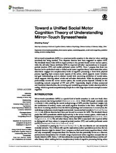
Euclidean distances. This version has been investigated by several authors (e.g., Shepard, 1958b; Takane & Shibayama, 1985). Nosofsky (1984, 1985b, 1986, 1987) generalized the model to account for categorization data, and he also considered other Minkowski distance metrics. In addition, Nosofsky (1985b, 1986) experimented with alternative similarity functions. In particular, he found that the Gaussian function n~ = exp(-d~ 2) provides better fits under certain experimental conditions (see also, Shepard, 1958a, 1986). Getty et al. (1979) investigated a generalization based on the weighted Euclidean distance model, and Appelman and Mayzner (1982) developed a version based on Krumhansl's (1978) distance-density model. Overall the model has provided good accounts of identification data. However, Takane and Shibayama (1985) found that the biasedchoice model (Equation 11) did a much better job accounting for the data of a complete identification experiment reported by Keren and Baggen (1981 ). Rather than use a distance-based similarity measure, Keren and Baggen (1981) replaced the d~ in Equation 12 with the dissimilarity measure of Tversky's (1977) feature-contrast model. The result is known as the unique-feature model. Smith (1982) pointed out several difficulties with this approach, and Takane and Shibayama (1985) found that the unique-feature model did a much poorer job in accounting for Keren and Baggen's (1981) numeral-naming data than either the biased-choice model or the MDS-choice model. A final important attempt to unify similarity and recognition, also based on the choice model, is Nakatani's (1972) confusion-choice model. Nakatani begins with a simple Euclidean distance model but assumes that computation of the distances is noisy. When a stimulus is presented, the distance from its representation to the representation of each stimulus in the ensemble is computed. If any of these distances exceeds a threshold level, the associated response alternative is eliminated from consideration. The subject is assumed to guess among the remaining alternatives in a fashion predicted by the choice model. None of these attempts have been completely successful. The MDS-choice models and Nakatani's confusion-choice model are based on geometric models of similarity and thus predict that perceived dissimilarity satisfies the distance axioms. Keren and Baggen's unique-feature model is based on a powerful similarity theory but has apparent difficulty in accounting for identification results. In the next section we describe a theory that we believe can successfully account for both the similarity and identification results. General Recognition Theory The general recognition theory, which motivates the similarity measure to be considered shortly, was described by Ashby and Townsend (1986) and Ashby and Gott (1988). However, because our purposes are somewhat different and because the theory may not yet be widely known, we briefly reintroduce it here. The general recognition theory assumes that the perceptual effect of a stimulus is random, but that on any single trial it can be represented as a point in a multidimensional space. With two dimensions, x and y, let j~(x, y) be the joint probability distribution (i.e., joint density function) of the perceptual effects elicited by stimulus Si. Figure 1 shows an example in which the
(a) fCx,y)
X
(b)
Cxy )
s
I
o S
"
s
U " , ,,"'*""" """QfB(x,y) s
Y s
X Figure 1. (a) The distribution of perceptual effects in an experiment
with two stimuli, SA and SB, that are each composed of two stimulus components, and (b) the contours of equal probability associated with the distributions of Figure la. (The dotted line is the optimal decision bound in a two-stimulusidentification experiment.)
stimulus ensemble contains two stimuli SA and Ss, each of which is constructed from the same two physical components. Figure la shows the distribution of the perceptual effects when the two stimuli are presented. Note that presentation of either stimulus could generate a perceptual effect anywhere in the perceptual space. The plane cutting through the two joint density functions describes the equal probability contours of the two distributions. Figure lb is a view of this plane from above. Every perceptual effect associated with any point on either circle is equally likely to occur (i.e., has the same probability density). Although the general recognition theory can account for both recognition and similarity, we begin by applying it to a twostimulus identification task. Suppose, as in Figure 1, that each stimulus is composed of a pair of stimulus components varying along the same two physical dimensions and that the subject is
SIMILARITY AND RECOGNITION shown either stimulus SA or SB and asked for an identification response. The presentation of a stimulus induces a perceptual effect (x, y). The decision process uses this perceptual effect to select one of the two responses RA or RB. The most accurate process selects the response associated with the stimulus most likely to have produced that perceptual effect. This effectively divides up the x, y space into two regions, one associated with each response alternative. The response is determined by the region into which the perceptual effect (x, y) falls. Thus a subject responding optimally never guesses. In Figure lb the dotted line marks the boundary between the two response regions. Any perceptual effect falling below the dotted line elicits an RB response, and any falling above the dotted line elicits an RA response. Ashby and Gott (1988) presented empirical evidence that at least for the kinds of stimuli considered here, subjects can place the boundary so performance (e.g., response accuracy) is approximately optimized. In so doing, they exhibit almost no variability in their response process. To maximize the probability of a correct recognition, the boundary is placed where the likelihood ratio equals one. Thus the optimal boundary is the set of points satisfying
l(x, y) = fA(X, y) = 1
A(x, y )
"
A response bias occurs if the boundary is set anywhere else. In this case the subject's decision rule is no longer optimal in terms of accuracy, although it may still maximize payoffs. (See Ashby & Gott, 1988, for a more thorough discussion of perceptual decision rules.) The most familiar version of this model assumes the perceptual distributions are multivariate normal. This special case, called the general Gaussian recognition model, is related to the Case I model of Thurstone's law of categorical judgment (Thurstone, 1927; see also Hefner, 1958; Torgerson, 1958; Zinnes & MacKay, 1983), but it can also be viewed as a multidimensional generalization of signal-detection theory (see, e.g., Green & Swets, 1966; Tanner, 1956; Wandell, 1982). The contours of equal probability of a bivariate normal distribution are always ellipses or circles. Their shape is determined by the variances and by the covariance (or correlation) parameters. ~ When the covariances are all zero, and the variances are all equal, the contours of equal probability will be circles. As the variances become unequal or a covariance arises, the contours of equal probability become ellipses. The general Gaussian recognition model is important because, as we will show, it contains the general Euclidean scaling model as a special case. On some trials there will be enough perceptual noise to cause the percept to fall into a region associated with the incorrect response. In particular, the probability of confusing SB with SA is given by
P(RBISA)= f f fA(x, y) dx dy, RB
where RB is the region in the x, y plane associated with response RB. Any factor that decreases the proportion of the SA perceptual distribution falling into the RB response region (and vice versa) will decrease the SA, SB confusability. One way to do this
129
is to increase the distance between the means of the two distributions, but decreasing the relevant variances will have the same effect. Thus, in the general recognition theory, the probability of a correct recognition is not necessarily monotonic with the distance between perceptual means. We are now ready to define similarity.
Perceived Similarity in the General Recognition Theory As mentioned previously, our initial hypothesis is that similarity and confusability covary. The more similar two stimuli, the more often they are confused. This does not imply, however, that similarity is the only factor affecting confusability. Response bias is also important. A subject with a strong bias toward responding RA will almost never confuse SB with S^ (i.e., P[RBISA] will be very low). In the absence of response bias, however, we begin by assuming that perceived similarity is proportional to the probability of a confusion. This assumption has a long history in the recognition literature. For example, it is made by the biased-choice model, which as we have noted has been the most successful model of the last 20 years at predicting the pattern of confusions in wide varieties of recognition experiments (see, e.g., Luce, 1977). Within the context of the general recognition theory it implies that
s(SA, SB) = k f f fA(x, y) dxdy,
(13)
where k is a positive constant and RB is the region in the x,y perceptual plane associated with response RB in an unbiased identification experiment. Extension to the n-dimensional case is straightforward. The constant k acts like the unit of measurement in a ratio scale and so can be set to one, without loss of generality. Ashby and Gott (1988) found that for the kinds of stimuli considered in the experiments that follow, subjects chose decision rules that were nearly optimal. Therefore throughout this article we will assume that the response regions specified in Equation 13 are determined by placing the decision bound where the likelihood ratio equals one. 2 In general, this requires the subject to integrate information from the various perceptual dimensions (e.g., Ashby & Gott, 1988). Keep in mind, however, that with some
In particular, the contours all satisfy
for some arbitrary constant c and where ~ and m are the m e a n and
variance on dimension i (i = x or y) and p is the correlation between the two variates. 2 A straightforward generalization of this definition would be to allow biased similarity judgments. Thus the decision bound implicit in Equation 13 need not be set where l(x, y) = 1. This kind of generalization does not equate identification and similarity because the bias process operating in the two tasks may be very different. Because the need to postulate response bias in judgments of similarity has not yet been demonstrated, we focus on the simpler unbiased Equation 13 definition of similarity in this article.
130
E GREGORY ASHBY AND NANCY A. PERRIN
(perceptually separable) stimulus components this may not be possible.In these cases,the response regions specifiedin Equation 13 might be determined by some other setof unbiased decision bounds (e.g.,those that are parallelto the coordinate axes; see Ashby & Gott, 1988). Thus, in the generalrecognitiontheory,the perceived similarity of stimulus SA to SB is naturallydefined as the proportion of the SA perceptual distributionfallingin the response region assigned to Rs in an unbiased two-choice recognitiontask. W e believe that Equation 13 provides a very good firstapproximation of perceived similarity.However, examples can be found in which confusabilityand similarityare not strictlymonotonic, and so we believethat a complete theory of perceived similarity must generalize Equation 13 somewhat. For example, celery, apples, and automobiles are never confused, and yet we judge celery and apples to be more similar than celery and automobiles(see Appendix A and Gati & Tversky, 1984, for other failures of the assumption). In Appendix A we present a generalization of Equation 13 that can account for this and many other examples in which similarityis not a strictlyincreasingfunction of confusability.The generalization is somewhat more complex than Equation 13, and for the applicationswe consider in thisarticle,itmakes virtuallyidenticalpredictions. In defining perceived dissimilarity,we assume only that itis inversely related to S(SA, SB). For example, one convenient measure of the dissimilarityOf SA tO SB (e.g.,Luce, 1963),is
d(SA, Sa) = -In S(SA, SB).
(14)
Equation 13 provides an unambiguous definition of similarity in the case where the stimulus ensemble contains two elements or objects. However, with three or more stimuli in the ensemble, several interpretations are possible. For example, consider the case of Figure 2 in which the ensemble contains stimuli SA, SB, and Sc. In a recognition task, the optimal and unbiased decision bounds are L~ and L 3 (i.e., these bounds maximize probability correct). Ifa sample falls above L~, the subject responds RA; if it fails between L~ and Z3, the subject responds RB; and if it falls below L3, then response Rc is made. Now consider how the general recognition theory defines the similarity Of SA tO Sc:
S(SA, Sc) = f f fA(x, y) dx dy. Rc Where is the optimal unbiased response region in this case? If the entire ensemble is considered, then the region is below the bound L3. But if one considers stimuli SA and Sc in isolation, then the region below the bound L2 is the optimal unbiased response region. We call the former a context-sensitive similarity model and the latter a context-freesimilarity model. Note that the context-sensitive general recognition theory predicts that the perceived similarity of SA to Sc is decreased by the presence ofSB. Tversky (1977) presented data supporting this prediction. When asked to make similarity judgments about pairs of countries, more subjects believed that the similarity of Austria to Sweden was greater than the similarity of Austria to Hungary when Poland was in the stimulus ensemble. However, when Poland was replaced by Norway, more subjects
,l L2 fA ),
fc X
Figure2. Contours of equal probability and possibledecision bounds for a three-stimulus identificationexperiment.
believed that the similarity of Austria to Hungary was greater than the similarity of Austria to Sweden. Norway is highly similar to Sweden (as SB is to Sc in Figure 2), and when it was added to the stimulus ensemble, the perceived similarity of Austria to Sweden decreased. Traditional geometric similarity models are context free because they predict that the similarity of SAto Sc is only a function of the distance between their perceptual representations and so is unaffected by how many or which other stimuli are in the ensemble. One way to make MDS models sensitive to context is to allow subjects to weight differentially the psychological dimensions, as in the weighted Euclidean model, in a manner that depends on stimulus context (e.g., Carroll & Chang, 1970; Getty et al., 1980; Nosofsky, 1986). In this model, adding a new stimulus to the ensemble causes the subject to readjust the amount of attention focused on each dimension, thereby effectively stretching some dimensions and shrinking others, and in so doing, changing the predicted similarities between all stimulus pairs. Krumhansrs (1978) distance-density model was another attempt to make geometric models context sensitive. For example, adding stimulus SB to an ensemble containing SA and Sc will not affect the distance between the SA and Sc representations, but it will affect the density around each representation and so, according to the distance-density model, will affect the perceived similarity Of SA to Sc. The general recognition theory of similarity can be formulated in either a context-free or a context-sensitive manner. With more than two stimuli, some additional assumptions are needed to define self-similarity in the context-free version (e.g., to select the appropriate decision bound). One possibility is to assume, as in geometric models, that all self-dissimilarities are zero. However, context is known to play an exceedingly important role in perceptual and cognitive processing (e.g., Garner,
SIMILARITY AND RECOGNITION 1962), and it has been shown to have large effects on human similarity judgments (Tversky, 1977). Thus any complete similarity theory must account for context. We stress that the general recognition theory provides a theory of perceived similarity. It predicts that similarity is determined by the overlap of perceptual distributions. As stimuli become more conceptual, high-level cognitive influences may start to play a greater role in judgments of similarity. For exampie, Gati and Tversky (1984) mentioned a case in which two stimuli that are related by a 180* rotation are judged to be more similar than two stimuli that are not related by a rotation but share more features in common. One possibility is that in the original perceptual space, the distributions associated with the stimuli sharing more common features had the greatest overlap but that cognitive intervention caused the subject to imagine a rotation of the percepts associated with the stimuli and that this operation led to a new space in which the distributions associated with the stimuli related by a rotation had the greatest overlap. If this hypothesis is correct, the stimuli sharing many common features should be judged more similar than the stimuli differing by a rotation in an experiment requiring speeded responses, because mental rotation requires extra processing time (e.g., Shepard & Metzler, 1971). Although both the general recognition theory and MDS theories postulate similar multidimensional spaces, these two classes of models have very different foundations. In MDS models, similarity is a fundamental construct. Indeed the psychological space could rightly be called a similarity space. In the general recognition theory, similarity is a derived construct. It depends on complicated relations between different perceptual distributions. In fact, the general recognition theory predicts that the task of judging perceived similarity will be very difficult for subjects because it requires them to do something roughly analogous to multiple integration. In addition, accurate judgments require fairly precise estimates of all parameters associated with the perceptual distributions. In many cases, for example in tasks in which subjects are required to respond after only a few presentations of novel stimuli, such estimates will not be available. How can a subject respond in such cases? If the subject does not have enough experience with the stimuli to estimate roughly the distributions of perceptual effects, then to fulfill the experimenter's instructions to judge similarity, the subject must make some assumptions about these distributions. For example, subjects might make the plausible hypothesis that all variances are equal and all correlations are zero. In this case, Lemma 1, which will be presented shortly, indicates that the predictions of the general recognition theory are equivalent to predictions of the simple Euclidean MDS model (in the absence of context effects). Thus one interesting prediction of the general recognition theory is that MDS models are more likely to fit data from experiments with artificial or unfamiliar stimuli. On the other hand, Ashby and Gott (1988) showed that subjects can detect correlations among stimulus components with fewer than 100 presentations, so humans might be very good at quickly estimating the necessary parameters.
Relation of the General Recognition Theory to M D S Models The general recognition theory of similarity appears to be related to traditional geometric models because increasing the
131
distance between the means of two perceptual distributions will often (but as we will show, not always) decrease the Equation 13 measure of similarity. In this section we show that the general recognition theory of similarity contains Euclidean MDS models as a special case. To derive the Euclidean metric exactly, it is necessary to assume a specific relation between similarity and dissimilarity. Let ~(z) = P(Z < z) be the standard normal cumulative distribution function. The equivalence mapping between the general recognition theory and MDS requires
d(SA, SB) = --2~-118(SA, SB)].
(15)
Note that as required, similarity and dissimilarity are inversely related under this assumption. The relation of the general recognition theory to MDS models of similarity that assume a Euclidean metric depends on the following result. The proof is given in Appendix B.
Theorem: Suppose perceived similarity and dissimilarity are related by
d(SA, SB) = - 2 ~ - I t s ( S A , SB)].
5
If the covariance matrix of the perceptual distribution associated with each stimulus equals
Z =[
trx2 Pxy0"xO'y] LPxyO'xO'y ~2 /'
27
then the context-free general Gaussian recognition model predicts d(SA, SB) = ' 2
2 (t*xA -- UxB)2
~x (1-Ox,)
1 [ 1 ]1/2 + O-y2(1 ,Oxy2)(~yA -- ~yB)2 -- 20.x2 (1 - ,Oxy2)l ]1/2 "11/2 X [ay2( 1 1 Oxy2)j pxy(/a,~ -/*,al)(/iyA --/*yii)J , (16) where, for example, tZ~Ais the perceptual mean associated with stimulus SA on dimension x. This theorem allows us to determine quickly the relation of the general recognition theory to Euclidean MDS models. For example, if 9 equals the identity matrix, I, that is, if a 2 = ay2 = I and p~y = 0, then Equation 16 reduces to Equation 1. We have proved the following.
Lemma 1: The simple Euclidean MDS model is a special case of the context-free general Gaussian recognition model in which all covariance matrices equal the identity and in which similarity and dissimilarity are related by d(SA, SB) = --2~-'[S(SA, SB)]. If ~x2 4:~y2 but pxy = 0, then Equation 16 reduces to Equation 2, where wi = 1/r for i = x or y. To ensure model testability, however, the weighted Euclidean MDS model and the general Euclidean scaling model both assume that the set of coordinates locating the stimulus representations is the same for all subjects.
132
E GREGORY ASHBY AND NANCY A. PERRIN
Thus the equivalent general Gaussian recognition model assumes that the set of means locating the perceptual distributions is the same for all subjects. These facts can be summarized as follows.
fA
L e m m a 2: The weighted Euclidean MDS model is a special case of the context-free general Gaussian recognition model in which the set of means locating the perceptual distributions is the same for all subjects and in which each covariance matrix for subject j equals
~-~j"~[1/oWXj21 / 0 2 1
9
In addition, perceived similarity and dissimilarity are related
by
fB
dj(SA, SB) = 2 ~-I[sj(SA, SB)]. The final lemma establishes the relation between the general Euclidean scaling model and the general Gaussian recognition model. L e m m a 3: The general Euclidean scaling model is a special case of the context-free general Gaussian recognition model in which the set of means locating the perceptual distributions is the same for all subjects and in which each covariance matrix for subjectj equals 1/(Wx/2 sin20j) sin20j)
~ J ---- -- COS
--
Oj/(WxjWy j
Oj/(WxjWy j sin20j) 1 1/(Wyj 2 sin20j) ]
COS
In addition, perceived similarity and dissimilarity are related
by dj(SA, SB) = - 2 '~-I[sj(SA, SB)]. These three results indicate that the general recognition theory can account for any similarity data generated by a Euclidean MDS model. They also point out the strong distributional assumptions of MDS models (e.g., that all covariance matrices are equal). By comparing Equation 16 with Equation 3 it becomes obvious that if the conditions of the theorem hold, then the parameters of the general Euclidean scaling model can be found from the parameters of the general Gaussian recognition model by
WXj :
~
1
1
Wyj : O'yj~i" -- Pxyj2 and COS Oj = --Pxyj. The dimension weights wx and ws are therefore inversely related to the standard deviations ax and a s. This relation fits nicely with the interpretation of wi as a measure of the relative attention allocated to dimension i. It is natural to suppose that the more closely a subject attends to a stimulus dimension the
Figure 3. Contours of equal probability for a case in which the general recognition theory predicts a violation of symmetry.
smaller the perceptual noise (e.g., Luce, Green, & Weber, 1976). Also note that these mappings provide justification for using the angle 0 as a measure of perceptual independence, because 0 = 90* if and only if pxy = 0, which in the special Gaussian case implies a statistical (and perceptual) independence of the perceptual effects x and y. Of course, the test is valid only if all the conditions of the theorem are met, that is, only if(a) perceived similarity is context free, (b) perceptual distributions are multivariate normal, (c) the variability on each perceptual dimension is the same for all stimuli, and (d) the degree to which the stimulus components are perceived dependently is the same for all stimuli. (See Ashby & Townsend, 1986, for a more thorough discussion of the relation of perceptual independence to dimensional orthogonality and to other related concepts.) When all covariance matrices are equal, the context-free general Gaussian recognition model is therefore equivalent to some Euclidean MDS model. As such, it is constrained by the usual distance axioms. However, when the covariance matrices are not all equal, the general recognition theory is not constrained by the distance axioms and so can account for data that falsify all geometric models of similarity. We illustrate this for each distance axiom in turn. Figure 3 illustrates a case in which the general recognition theory predicts a violation of symmetry. The overlap of the SA perceptual distribution into the Rs response region is greater than the overlap of the SB distribution into the RA region, and so the general recognition theory predicts that d(SB, SA) > d(SA, SB). Appendix C contains parameter values corresponding to the Figure 3 model and gives specific dissimilarity predictions of the general recognition theory. According to the general recognition theory, there are three primary situations in which symmetry fails. The first occurs when a large difference exists between the perceptual corre-
SIMILARITY AND RECOGNITION lations associated with each stimulus. This is the situation in Figure 3. The perceptual correlation in Distribution A is negative and the correlation in B is positive. In this case d(Se, SA) > d(SA, SB), but the inequality could reverse if the perceptual means were changed. In general, there is no way to predict the direction of the inequality by examining the correlations alone. The second situation that leads to a violation of symmetry occurs when there are differences in the amount of perceptual variability along any given dimension. An example can be found ahead in Figure 8. The context-free general recognition theory predicts d(Se, SA) > d(SA, SB). The general recognition theory predicts that the larger the variance, the greater the overlap into neighboring response regions and so the greater the similarity. Therefore a general rule of thumb is that if the perceptual variability associated with SA is greater than the variability associated with Se, then d(Se, SA) > d(SA, Se). Finally, the third situation condusive to violations of symmetry results because of context effects. Again in Figure 8, because Se and Sc are so similar, in the context-sensitive general recognition theory the response region associated with Se is very small. Therefore the amount of the SA distribution falling in the Re response region will be small, and consequently, as SB and Sc become more similar, the effect of the differences in perceptual variability will eventually be overcome and d(SA, Se) > d(Se, SA). In general, if a stimulus Si is associated with a very small response region, then the perceived similarity of Si to each of its neighbors will be greater than the perceived similarity of each neighbor to Si. Several of these factors may contribute to the asymmetry found by Tversky (1977) when he asked subjects to evaluate the similarity of North Korea and Red China. First, for many people North Korea is very similar to several other countries (e.g., South Korea and North Vietnam) and thus would be associated with a very small response region in an unbiased identification task. Second, for many people North Korea is a more vague and poorly defined concept than Red China, and so the variability associated with the mental representation of North Korea should be greater than the variability associated with the concept of Red China. As we have shown, both of these factors will tend to cause the perceived similarity of North Korea to Red China to exceed the perceived similarity of Red China to North Korea. Note that the general recognition theory is able to account for violations of symmetry without having to postulate context effects. Krumhansl's (1978) distance-density model can also account for symmetry violations, but only by appealing to context. Because of this, a violation of symmetry when the stimulus ensemble contains only two stimuli falsifies the distance-density model but not the general recognition theory. Note also that the general recognition theory predicts different self-dissimilarities for stimuli SA and SB in Figure 3. Because a smaller proportion of the SA perceptual distribution lies in its own response region (i.e., the RA region), it predicts that the self-dissimilarity of Se is less than the self-dissimilarity of SA (see Appendix C for specific numerical predictions). In fact, this is a consequence of the Equation 13 definition of similarity. With two stimuli in the ensemble, the general recognition theory predicts that if S(SA, SB) > S(SB, SA) then S(SB, Se) > S(SA, SA). If our Red China-North Korea example is correct, we
133
fB Y
I
X Figure4. Contours of equal probability for a case in which the general recognition theory predicts a violation of the triangle inequality.
might therefore expect people to judge the self-similarity of Red China to be greater than the self-similarity of North Korea. Figure 4 contains an example in which the general recognition theory predicts a violation of the triangle inequality (see Appendix C for specific numerical predictions). In this case the similarities between SA and SB and between SB and Sc are both high, and so the dissimilarities d(SA, SB) and d(Sa, Sc) are fairly small. However, in Figure 4 there is very little overlap between the SA and Sc perceptual distributions, and so d(SA, Sc) is large. In fact, in many cases it will be larger than the triangle inequality predicts (i.e., greater than d[SA, Se] + d[SB, Sc]). Note that this result does not depend on context. Because the general recognition theory is not constrained to predict the triangle inequality, we would also expect it not to be constrained by the corner inequality. In this case, intuition proves correct. Appendix C lists parameter values for which the general recognition theory predicts a violation oftbe corner inequality. The general recognition theory predicts that violations of minimality must be due to context effects. Even in the presence of context the theory predicts minimality to be only rarely violated. For if it is, some stimulus Se must be more similar to SA than SA is to itself. In the two stimulus case this implies that in the absence of any response bias, recognition performance should satisfy
P(RBISA) > P(RAISA).
~-(-
NO matter how difficult the discrimination, with only two re-
sponse alternatives, we expect an ideal observer to be correct at least half the time. The general recognition theory can account for violations of minimality in the presence of context. A one-dimensional example is given in Figure 5 (Appendix C contains numerical details). Because the three stimuli are so similar, the proportion of
134
F. GREGORY ASHBY AND NANCY A. PERRIN
RA
RB
Rc
fB
{
.
.
.
.
.
.
.
.
.
i
.
.
.
.
.
.
.
I
.
.
.
.
.
.
.
.
.
I
X
Figure 5. Perceptual distributions and decision bounds for a case in which the general recognition theory predicts a violation of minimality.
the SB perceptual distribution falling into the RA response region is greater than the proportion falling into the RB region, and so the general recognition theory predicts that the dissimilarity of SB to SA is less than the self-dissimilarity of SB. Figure 5 suggests that minimality might be violated in something like the following situation. Suppose the stimuli are three monochromatic lights (e.g., 550 nm) differing only in intensity. If the three intensities are all near threshold (to guarantee large perceptual variances) and very close together, then identification of SB, the middle intensity, will be very difficult. If it is so difficult that in the absence of bias
P(RAISB) > P(RBISB), then the general recognition theory predicts that when similarity judgments are collected, minimality will be violated. In summary, we have seen that the general recognition theory contains Euclidean MDS models as a special case, including those that allow differential weighting of potentially oblique psychological dimensions. Any data that can be accounted for by the general Euclidean scaling model can therefore be perfectly fit by some context-free general Gaussian recognition model. On the other hand, we have also seen that the general recognition theory is much more general than the Euclidean MDS models, because it can account for violations in each of the distance axioms.
sure. As we will show in the discussion of Experiment 1, this difference appears to be fundamental. Determining the formal relation of the general recognition theory to Tversky's (1977) feature-contrast model poses some difficulties. For example, MDS models and the general recognition theory both postulate perceptual spaces with continuous psychological dimensions, but the feature-contrast model is stated in terms of what are presumably discrete features, and no geometric perceptual space is defined. Some indication of their relation can be obtained by asking whether the general recognition theory is constrained by the three axioms that define a monotone proximity structure (dominance, consistency, and transitivity; see Equations 8-10), and that are predicted by a large class of feature-contrast models. As with the distance axioms, it turns out that the general recognition theory is not constrained to predict any of these axioms. First, consider dominance. Figure 6 illustrates contours of equal probability for which the general Gaussian recognition model predicts that dominance will be violated (see Appendix C for numerical details). The key component of Figure 6 is the positive correlation between perceptual components. Ashby and Townsend (1986) associated such a correlation with a perceptual dependence. In this case the perceptual dependence causes the overlap of the SB and Sc perceptual distributions to exceed the overlap of the SA and Sc distributions and the overlap of the SA and SB distributions. Thus, in Figure 6, the two-dimensional dissimilarity is less than either one-dimensional dissimilarity. Perrin and Ashby (1986) reexamined the data of an experiment reported by Dunn (1976; see also Dunn & Harshman, 1982), in which similarity judgments were collected on pairs of plastic blocks that differed in size and weight. Because of the size-weight illusion, larger objects are perceived to be heavier than smaller objects of the same mass, and so a perceptual dependency of the sort illustrated in Figure 6 exists between these
C
Relations to Other Models Structurally, the general recognition theory closely resembles Nakatani's (1972) confusion-choice model and the probabilistic MDS models described earlier (Ennis & Mullen, 1986; Luce & Galanter, 1963; MacKay & Zinnes, 1981; Mullen & Ennis, 1987; Suppes & Zinnes, 1963; Zinnes & MacKay, 1983). In all cases a multidimensional probabilistic stimulus representation is postulated. However, only the general recognition theory equates perceived similarity with distributional overlap. The other models all involve the computation of some distance mea-
Figure 6. Contours of equal probability for a case in which the general recognition theory predictsa violation of dominance.
SIMILARITY AND RECOGNITION
Y G
lower level on dimension y but that it decreases on dimension x for the upper level on dimension y. This is certainly not a phenomenon we ordinarily expect, and so the general recognition theory predicts consistency to be more empirically robust than, say, dominance. However, it is possible to construct stimulus ensembles that might possess this property. For example, consider an experiment in which subjects are asked to judge the similarity of certain color mixtures. Suppose we create the mixtures by adding a monochromatic light to white. Let the first dimension correspond to the amount of white light and the second dimension correspond to the wavelength of the monochromatic light. If we pick these two wavelengths to be 460 nm (indigo) and 520 nm (green), the resulting perceptual space should have the desired property. MacAdam (1942) estimated standard deviations of the wavelengths of indiscriminable colors in a two-color discrimination experiment and found that as more white is added to indigo, the standard deviation increases, but that as more white is added to green, the standard deviation decreases. The general recognition theory predicts that violations of consistency are therefore likely in this experiment. Perceptual distributions for which the general recognition theory predicts a violation of transitivity are shown in Figure 8 (again, numerical details can be found in Appendix C). Note that the four stimuli differ on only one dimension. Perceptual variability is small for the center two stimuli and large for the endpoint stimuli. Transitivity is violated, but only in the context-sensitive general recognition theory.
H
q
P A
B a
b
c
d
135
,x
Figure 7. Contours of equal probability for a case in which the general recognition theory predicts a violation of consistency.
two components. As predicted by the general recognition theory, dominance was found to be consistently violated. Figure 7 illustrates an instance in which the general Gaussian recognition model predicts a violation in consistency (Appendix C contains numerical details). The critical feature of this example is that variability increases on the x dimension for the
B
C
f
X Figure 8. Perceptual distributions for a case in which the general recognition theory predicts a violation in transitivity.
136
F. GREGORY ASHBY AND NANCY A. PERRIN
SA
SB
Figure 9. Prototypical stimuli from Experiment 1.
The Figure 8 perceptual distributions might arise under something like the following conditions. Consider pure tones differing only in frequency. Suppose, through some method, subjects are induced to focus attention on a certain band of frequencies. Perceptual distributions like those in Figure 8 should result if the center two stimuli are contained within this band and the two endpoint stimuli lie above and below its edges. These counterexamples indicate that the general recognition theory and the feature-contrast model are empirically distinguishable. The experimental results that follow, however, are meant to test basic predictions of the general recognition theory and are not specifically meant to discriminate it empirically from the feature-contrast model. Such a task is beyond the scope of this article (but see Perrin & Ashby, 1986). Experiment 1 The first experiment was designed to test the basic prediction of the general recognition theory that distributional overlap is the key predictor of perceived similarity. Ideally, we desire an experimental technique that permits precise control of a subject's perceptual distributions. We could then vary distributional overlap across experimental conditions while holding constant, say, the distance between perceptual means. Of course, in most experimental paradigms the perceptual representations and therefore their distributions are not directly observable, and so they are difficult to experimentally manipulate. Ashby and Gott (1988) developed an experimental paradigm, called the general recognition randomization technique, that attempts to approximate the unobservable perceptual space with an observable stimulus space. The technique begins with a pair ofprototypical stimuli. Like Ashby and Gott, we chose stimuli composed of vertical and horizontal line segments joined at an upper left corner. The prototypes of Experiment 1 are shown in Figure 9. Note that they differ only in the lengths of their component line segments. In the general recognition randomization technique, each stimulus is associated with a specific bivariate distribution in which the dimensions correspond to horizontal and vertical line length. The Figure 9 prototypes correspond to the means of the stimulus distributions. For example, the stimulus SA distribution has a small horizontal mean and a large vertical mean. On each trial a sample (i.e., a horizontal and a vertical length) is randomly drawn from one of the two stimulus distributions. A
stimulus is then constructed with horizontal and vertical line lengths that agree with the sample and is then presented to the subject. Note that the subject may never be shown the Figure 9 stimuli exactly. In the experiment that follows, stimulus contrast was high, and displays were response terminated, so that internal noise was minimized. The perceptual dimensions will not agree with the physical dimensions, but if Stevens or Fechner were correct, they should be monotonically related, and the perceptual distributions should be nearly monotonically related to the actual stimulus distributions. Experiment 1 was divided into blocks. Each block consisted of 50 categorization trials to enable subjects to learn the stimulus distributions and then a single similarity judgment (on a 7-point scale). On each categorization trial subjects were first shown a stimulus created by random sampling from one of two bivariate normal distributions labeled A and B and were then asked to categorize it as a member of Class A or Class B. They were given feedback after every trial. At the end of each block subjects were asked to judge the similarity of the two groups o f stimuli they were shown during that block (i.e., to judge the similarity between the Category A exemplars and the Category B exemplars seen during that block). The experiment contained three conditions: a small overlap condition, a moderate overlap condition, and an extreme overlap condition. The means of the two distributions remained unchanged across conditions. Distributional overlap was manipulated by varying the variances and covariances. The contours of equal probability for the three conditions are shown in Figure 10. The diagonal line represents the optimal decision boundary for the categorization task. Probability correct is maximized by responding A to any sample falling above this diagonal and otherwise responding B. Note that the same bound is optimal in all three conditions, and thus subjects need not change decision rules when shifting from one condition to another. Ashby and Gott (1988) showed that under these conditions and without any coaching, subjects quickly adopt and very consistently apply the optimal rule. The variances and covariances were selected so that an ideal observer could correctly categorize 95% of the stimuli in the small overlap condition, 80% in the moderate condition, and 65% in the extreme condition. Even so, total variation was the same in the small overlap and the extreme overlap conditions (i.e., the variances were identical). The only difference between the two conditions was the covariance term. Note that in this task, subjects were asked to judge category similarity rather than stimulus similarity. First, we believe a study of category similarity is of interest in its own right. Judgments of category similarity account for a large percentage of human similarity judgments. People are very comfortable judging the similarity of Bach's music to Vivaldi's, Van Gogh's painting to Monet's, Szechwan cuisine to Mandarin, and Vonnegut's writing to Barth's. Each of these are judgments of category similarity. Second, although the general recognition theory was developed initially as a theory of stimulus similarity, we believe that subjects use the same basic processes whether judging the similarity of two single stimuli or two stimulus categories. Thus we feel that the results of Experiment 1 are also rele-
SIMILARITY AND RECOGNITION
k
Small overlap condition
k
Moderate overlap condition
k
137
vant to the study of stimulus similarity. If the general recognition theory is correct, then even in experiments where subjects are asked to judge the similarity of two single stimuli, repeated exposure to each stimulus does not always elicit the same percept (because of perceptual noise, a shifting focus of attention from one set of stimulus dimensions to another, etc.). Instead, many percepts are associated with the same stimulus. Thus when judging the similarity of one stimulus to another, the subject must judge the similarity of one set of percepts with another set of percepts, exactly as in judgments of category similarity. When deriving the Experiment 1 predictions for the various models, it is necessary to generalize them to account for category similarity. In the case of the general recognition theory, this is straightforward. Although a small amount of perceptual noise will be associated with each stimulus sample, most of the variability within each category is due to experimental manipulation of the stimulus distributions. Thus the general recognition theory predicts similarity to be greatest in the extreme overlap condition and least in the small overlap condition. 3 It turns out that there are several ways to generalize MDS models to predict category similarity. An especially simple model predicts that judgments of category similarity should behave the same as judgments of stimulus similarity. In other words, each category is represented by a single point in the perceptual space and judgments of category similarity are based on the distance between category representations. This model is a straightforward generalization of prototype models of categorization (e.g., Ashby & Gott, 1988; Homa, Sterling, & Trepel, 1981; Posner & Keele, 1968, 1970; Rosch, 1973; Rosch, Simpson, & Miller, 1976), and so we will refer to it as the prototypebased MDS model. Because the stimulus means are identical in all three Experiment 1 conditions, their perceptual representations should also be identical, no matter what the relation between the physical and perceptual dimensions (as long as it is deterministic). Thus prototype-based MDS theories predict perceived similarity to be the same across conditions. Of course, if perceived similarity is found to vary across conditions, the prototype-based MDS model might still be useful as a data-reduction technique. An MDS computer program could account for such results by allowing the Category A and B perceptual representations to change across conditions, in spite of the absence of any change in the stimulus parameters on which prototype-based MDS theories assume perceived similarity to depend. Other MDS type models will be discussed later. The purpose of Experiment 1 is to demonstrate the importance of distributional overlap as a predictor of perceived similarity and to illustrate the power of the general recognition ran-
3 Specifically,under these experimental conditions, the general recognition theory predicts
s(A, B) = s(B, A) =
fff oo
Extreme overlap condition Figure 10. Contours of equal probability representing the three conditions of Experiment 1.
fA(x, y)dy dx, oo
where fA(X, y) is the bivariate normal probability density function. It can be shown that this integral equals .95 with the stimulus parameters of the small overlap condition, .8 in the moderate overlap condition, and .65 in the extreme overlap condition.
138
E GREGORY ASHBY AND NANCY A. PERRIN
domization technique as a tool for manipulating distributional overlap.
Table I
Population and Sample Valuesfor Experiment I
Subjects. Eleven Ohio State Universitystudents enrolled in an introductory psychology course participated in the study for partial fulfillment of course requirements. Apparatus. A Data General Nova IV computer generated the stimuli, which were shown on an HP 1332a video displayusing a MEGATEK5000 graphics package. The video display had a resolution of 4096 • 4096. Subjects responded to stimuli by pressing buttons on a keyboard. Procedure. We began each experimental session by displaying the prototype stimuli (shown in Figure 9) along with their category labels. This phase was followedby seven blocks each consisting of 50 categorization trials and a single similarity judgment. On each categorization trial, one of the two stimulus classes(A or B) was randomly selected. A specific stimulus was generated by sampling from one of two bivariate logistic distributions and was then presented to the subject. The logistic was chosen because its shape is very similar to the normal distribution, but it has a simple closed form expression for its cumulative distribution function. Subjects were instructed to respond A or B on a keyboard according to which class they thought the stimulus belonged. Accuracy was stressed much more than speed. Subjects were told that it was impossible to respond with perfect accuracy and so not to let an occasional incorrect response discourage them. After a response was made the screen was blank for 1 s and then feedback was given as to which response was correct. The feedback appeared on the screen for 1 s and was followed by a 1-s pause before the onset of the next trial. A new condition (small, moderate, or extreme overlap) was selected for each block of 50 trials. To ensure rapid learning of the optimal decision rule, the first block was always the small overlap condition. Followingthis block the subjects were asked if they had any questions about the procedure. In the followingsix blocks, each of the three conditions appeared twice. Subjectswere given no information about the differencebetween blocks. The order of the blocks was controlled to eliminate possibleconfounding owing to ordering effects. At the end of each block, subjects were asked to judge the similarity of the two stimulus classes in that block by pressing one of seven buttons on a keyboard. Subjects were told that 7 meant the two classes were very similar and 1 meant they were very dissimilar. Before the beginning of the next block there was a 30-s rest period followedby a signal displayed on the screen to indicate the onset of the new block. The first block was considered practice (ineluding the first similarity judgment) and was not included in the data analysis.
Results and Discussion Table 1 shows the population and sample means, standard deviations, and correlations for the three conditions. Subjects averaged 91% correct on the categorization trials in the small overlap condition (where 95% was optimal), 78% correct in the moderate condition (where 80% was optimal), and 67% correct in the extreme overlap condition (where 65% was optimal). Therefore, overall, subjects were very nearly optimal. In fact, performance slightly exceeded optimal in the extreme overlap condition but only because, 0y chance, the stimuli actually presented to the subjects were slightly easier to classify than predicted (compare population and sample means in Table 1). The near-optimal performance of subjects in all three conditions is
Moderate overlap
Small overlap
Method Variable SA #x #y ~x ~y Pxy SB #x t~ ~x 9y o~
Population
Sample
POPulation
400 500 133 133 .896
389 486 140 144 .885
500 400 133 133 .896
496 399 126 124 .876
Extreme overlap
Sample
Population
Sample
400 500 84 84 0
391 495 85 84 .053
400 500 133 133 --.896
384 507 139 136 --.793
500 400 84 84 0
494 401 95 82 -.037
500 400 133 133 -.896
502 398 127 128 -.885
Note. The units here are arbitrary screen units in which there are about 270 units per degree of visual angle.
strong evidence that they understood the task and that they accurately learned at least the means of the stimulus distributions. The median of the two similarity judgments for each subject in each condition was computed, and the results were analyzed using the Wilcoxon Signed Rank Test. The results indicate that subjects judged the stimuli in both the extreme overlap condition and the moderate overlap condition as significantly more similar than the stimuli in the small overlap condition (p < .05 in both cases). In addition, the median for the moderate condition was less than the median for the extreme condition, but not significantly so. We suspect that this latter nonsignificance may be due to the higher-than-expected categorization performance in the extreme overlap condition. Overall, the data support the predictions of the general recognition theory. Because each condition used exactly the same prototypes, these results clearly show that perceived similarity is not simply a function ofinterprototype distance, no matter how distance is measured. If we try to examine the predictions of Krumhansl's (1978) distance-density model or Tversky's (1977) feature-contrast model, we encounter some ambiguity. Both of these models were developed to account for stimulus similarity, and it is not obvious how they might be generalized to account for category similarity. The obvious ploy of representing each category by its prototype and then using the distance-density model or the feature-contrast model to determine the similarity between prototypes fails for the same reason the prototype-based MDS models fail. The prototypes are the same in the three conditions, and therefore similarity should also be the same. Although the results of Experiment 1 cannot be predicted by prototype-based MDS models, another large class of MDS models assumes that instead of representing a category simply by its prototype, categories are represented by the individually stored exemplars. There are two versions of these exemplarbased MDS models. The first assumes that perceived similarity is based on the average distance between all samples in one stimulus class and all samples in the other (Homa et al., 198 I; but see also Ennis & Mullen, 1986; Luce & Galanter, 1963; MacKay
SIMILARITY AND RECOGNITION & Zinnes, 1981; Suppes & Zinnes, 1963; Zinnes & MacKay, 1983). The second version, proposed by Nosofsky (1986; see also Medin & Schaffer, 1978), assumes that perceived similarity is based on the average similarity between all samples in one stimulus class and all samples in the other (where similarity = exp[-distance]). Analytic predictions are extremely difficult to derive for the exemplar-based models because with the design of Experiment 1, they assume the subjects base their similarity judgments on the mean of 25 • 25 = 625 values (either similarities or distances, depending on the model). Therefore to generate predictions, we performed Monte Carlo simulations. First, to test the average distance hypothesis, 1,000 samples were drawn randomly from each stimulus distribution for each of the three experimental conditions, and then the average Euclidean distance was computed between each sample of one distribution and every sample of the other. Thus, 1,000,000 distances were computed to obtain each predicted average Euclidean distance. Five replications were performed. The means of the five resulting average Euclidean distances were 23.41 for the small overlap condition, 17.95 for the moderate overlap condition, and 21.68 for the extreme overlap condition. Ttests indicated that each of these differences was statistically significant (p < .01). Thus the average-distance hypothesis predicts that perceived similarity is greater in the moderate overlap condition than in the extreme overlap condition. This prediction was not supported by the data.* It indicates that the average-distance exemplar-based MDS model makes predictions different from the general recognition theory and that the model predicts that similarity is not monotonic with confusability. To generate predictions of the average-similarity exemplarbased MDS model, 200 samples were randomly drawn from each stimulus distribution in the three experimental conditions, and then the average similarity was computed between each sample of one distribution and every sample of the other. Thus 40,000 similarities were computed to obtain each predicted average similarity. This process was repeated 8 times. The means of the eight average similarities were .40 • 10-5 for the small overlap condition, 3.27 • 10-5 for the moderate overlap condition, and 5.92 • 10-5 for the extreme overlap condition. Ttests indicated that each difference was statistically significant (p < .01). Thus the average-similarity exemplar-based MDS model makes the correct ordinal predictions. It is therefore sensitive to second-order distributional parameters such as variance and correlation. Both the general recognition theory and the average-similarity exemplar-based MDS model are able to account for the similarity results of Experiment 1. In an effort to further discriminate between the models, we also might examine their ability to account for the categorization results of Experiment 1. Although the average-similarity exemplar-based MDS model is strictly a similarity theory, Nosofsky (1986) generalized it to account for categorization data by conjoining it with the MDSchoice model. The accuracy of the subjects in Experiment 1 seems to support the prediction of the general recognition theory that subjects employed the optimal decision bound of Figure 10. However, a more detailed analysis is needed. Ashby and Gott (1988) reported the results of several experiments using the general
139
recognition randomization technique in conjunction with the Figure 9 prototypes. One of these used the moderate overlap stimulus distributions of Experiment 1. As in Experiment 1, the subjects in the Ashby and Gott experiment responded nearly optimally. A more detailed analysis, however, indicated that as predicted by the general recognition theory, subjects used deterministic decision rules. In other words, for each sample falling above the Figure 10 decision bound, subjects virtually always responded A, and for each sample failing below, they almost always responded B. The average-similarity exemplar-based MDS-choice model predicts a gradual increase in the probability of responding A as samples move from lower right in Figure 10 (long horizontal and short vertical) to upper left (short horizontal and long vertical). Therefore, although this powerful model can account for the similarity results of Experiment 1, it cannot account for the categorization results. Still another possible interpretation of the results of Experiment 1 is that similarity judgments are based, not simply on interprototype distance, but rather on some standardized distance measure, such as the signal detectability measure, d'. To compute a standardized distance measure for each of the three conditions of Experiment 1, one might divide the interprototype distance by the average variation within the two stimulus distributions along the chord joining the two means. Because this dissimilarity measure is sensitive to both distributional location parameters (i.e., means) and shape parameters (i.e., variances and covariances), we expect its predictions to mimic those of the general recognition theory more closely than do the predictions of models that are sensitive only to distributional location (as, e.g., prototype-based MDS models). In fact, with the stimulus distributions of Experiment 1, the variation along the chord connecting the means tends to increase with distributional overlap, and so both the general recognition theory and standardized distance models make exactly the same ordinal predictions. The two theories are not equivalent, however, and it is possible to find experimental conditions in which they make divergent predictions. Experiment 2 was designed to test between the two theories. One could argue that the results of Experiment lare not very interesting because they only show that the more confusable a pair of categories, the more similar they are. This seems an obvious prediction. Of course, a good theory should predict the obvious. The point of Experiment 1 was to show that many of the popular similarity theories fail to make the obvious prediction. For example, the only difference between the extreme and the small overlap conditions was in the sign of the horizontalvertical correlation. In the small overlap condition the correlation was positive, whereas in the extreme overlap condition it was negative. Yet this one change had a large effect on perceived similarity. Very few similarity theories explicitly address such perceptual dependencies. Experiment 2 The purpose of this experiment was to decide whether distributional overlap or a standardized distance measure is a better 4 Of course, the nature of our Monte Carlo study limits this conclusion to the Euclidean distance metric and does not rule out the possibility that the average-distancehypothesiscould account for these results if some other distance measure is used.
140
F. GREGORY ASHBY AND NANCY A. PERRIN
RA
RB
RA
i
$00
200
UO0
500
SO0
700
BOO
HOnIIONTRL LENGTH
Figure 11. Distributions of stimulus samples and optimal decision bounds for Experiment 2.
predictor of perceived similarity. As previously mentioned, in many cases the predictions of the two theories will ordinally agree. An exception occurs when the perceptual distributions have identical means but different variances. A one-dimensional example is illustrated in Figure 11. In this case, because the prototypes are identical, the standardized distance between means is zero, regardless of the variances. If performance depends on a standardized distance measure, then subjects should not be able to discriminate between the two stimulus classes of Figure 11. Categorization should be at chance levels. On the other hand, because of the different variances, the general recognition theory predicts that categorization, although imperfect, can be significantly above chance. The optimal decision bounds are indicated by the dotted lines in Figure 11. If subjects respond RA tO any sample falling in either the left or the right regions, and RB tO any sample falling in the center region, their performance will be optimized. Exactly how much better than chance they will perform depends on the ratio of the variances. If the ratio is extreme enough, virtually perfect performance is possible. In fact, the only conditions for which the general recognition theory predicts that subjects can perform at no-better-than-chance levels occurs when the stimulus distributions are identical. Experiment 2 used the same design as Experiment 1. The stimuli were horizontal line segments sampled from the onedimensional distributions of Figure 11. Subjects were instructed to classify the stimulus samples as members of either Class A or Class B. Similarity judgments were not collected. The variances of each stimulus distribution were selected so that an ideal observer could correctly classify 80% of the stimulus samples.
Method Subjects. Four Ohio State University students in an introductory psychology course participated in the experiment as partial fulfillment of their course requirements. Subjects were recruited for a l-h session on each of 2 days, however, they were told that they need not return for
the second day if their proportion correct on the first day was greater than .75. Stimuli. Stimuli were horizontal line segments that differed in length. They were computer generated and displayed on the same equipment used in Experiment 1. Stimulus samples were generated in the same fashion as in Experiment 1 but by random sampling from one of two univariate logistic distributions. Both distributions had a mean of 500 screen units (where as in Experiment 1 there were approximately 270 units per degree of visual angle). Distribution A had a standard deviation of 125 units and Distribution B had a standard deviation of 23 units. Procedure. On each trial, one of two stimulus classes (A or B) was randomly selected. A specific stimulus was then generated by random sampling from the appropriate distribution and was presented to the subject. Subjects responded A or B on a keyboard according to which class they thought the stimulus belonged. Subjects were told that an "expert" would be correct about 80% of the time. Accuracy was stressed much more than speed. Stimulus displays were response terminated and were followed by feedback showing the correct response. There was a 3-s pause between trials. On each day, the first 100 trials constituted a practice session that allowed subjects to become familiar with the two stimulus distributions. After the practice session, subjects were asked if they had any questions about the procedure before the experimental blocks began. Both the practice and the first experimental block were preceded by prototypes of each of the two stimulus classes (i.e., the distribution means, which in this case were identical). Each appeared 5 times. There were four experimental blocks, each with 75 trials, and there was a 30-s pause between blocks to allow subjects to rest. On each day of the experiment, every subject participated in a total of 400 trials (100 practice and 300 experimental).
Results and Discussion The proportion of correct responses for the 4 subjects was .77, .75, .75, and .73, respectively. Note that in each case, performance was significantly above chance. In fact, because an ideal observer would be correct only with probability. 8, all subjeers responded at near-optimal levels, and one subject achieved this level by the end of the first day. The general recognition theory nicely accounts for the results of this experiment. It suggests that subjects classify a stimulus sample into the category of which it is most likely a member. With the stimulus distributions of Experiment 2, this strategy divides the perceptual dimension into three regions, two associated with response RAand one with response RB. One plausible interpretation of this rule is that following its consistent application, subjects may actually believe they are dealing with three stimulus categories, two that are assigned response RA and one that is assigned response RB. With the stimulus distributions of Figure 11, the standardized distance between prototypes is zero, yet subjects were able to classify the stimulus samples almost as accurately as an ideal observer. This indicates that standardized distance is not a perfect measure of human perceptual performance. Because the stimulus distributions in Figure 11 have the same prototypes, the results of Experiment 2 also contradict the predictions of prototype-based MDS models. Exemplar-based MDS models can predict better than chance performance, but a more detailed analysis is needed to determine whether these models can account for the near-optimal response levels of the Experiment 2 subjects.
141
SIMILARITY AND RECOGNITION
Another possible interpretation of these results is that subjects compute the distance (i.e., the difference in perceived length) from a given sample to the prototype and respond RB if this distance is small and RA if it is large. Although this interpretation is consistent with the Experiment 2 results, it is not consistent with the results of Experiment 1. As we saw, theories based on the assumption that subjects compute distances incorrectly predicted the ordinal relations between the similarity judgments of the three conditions of Experiment 1. In the first two experiments we concentrated on the ability of the general recognition theory to account for similarity and categorization data. However, one of the strengths of the general recognition theory, which we feel is very important, is its ability to also account for the results of identification experiments. Experiment 3 In this section we focus on the ability of the general recognition theory to account for recognition performance by fitting it to data from a complete identification experiment reported by Townsend, Hu, and Ashby (1980, 1981). We will then use the resulting parameter estimates to examine the model's stimulus similarity predictions. In addition, we will compare its ability to account for the identification data with the ability of some competing models, specifically the biased-choice model, two versions of the Euclidean MDS-choice model (one with an exponential similarity function, ~ = exp[-d~], and one with a Gaussian function, ~ = exp[-dij2]), the city-block MDS-choice model, and the unique-feature model developed from Tversky's (1977) feature-contrast model (by Keren & Baggen, 1981; Smith, 1982; Takane & Shibayama, 1985). In the Townsend et al. (1980, 1981) experiment, two levels (presence and absence) of two stimulus components (a horizontal and a vertical line segment) were factorially combined to create four stimuli. If we denote the horizontal feature as H and the vertical feature as V, then the four stimuli were VH (both features present), V (only the vertical feature present), H (only the horizontal feature present), and ~ (neither feature present). On each trial, one of these four stimuli was randomly selected and then tachistoscopically shown to the subject, who then made an identification response. In one condition, the components of stimulus VH were physically connected (the nongap condition), and in another condition they were separated by a gap (the gap condition). Four subjects participated in the experiment. Every subject was shown each stimulus a total of 150 times in each condition.
Competing Models As mentioned earlier, the model that has been most successful in predicting a wide variety of confusion matrices is the biasedchoice model of Fxtuation I 1. A good test of the general recognition theory's ability to account for recognition data, therefore, would be to compare its performance with the biased-choice model. Each 4 • 4 confusion matrix has 12 degrees of freedom. The biased-choice model has nine free parameters--six similarities and three bias parameters--leaving 3 degrees of freedom to test the model. Some simplifying assumptions are needed to fit the MDS-
choice models and the unique-feature model to these data. First, in the case of the MDS-choice models, because the stimuli are composed entirely of horizontal and vertical line segments, it is reasonable to assume that the perceptual space is two dimensional. Call the dimension associated with the horizontal component h, and let v be the dimension associated with the vertical component. Because there are four stimuli, there will therefore be eight coordinate values. However, without loss of generality we can arbitrarily fix the coordinates of stimulus r at (0, 0), and in the Euclidean models we can set the v coordinate of stimulus H to 0. This leaves five free coordinate parameters in the Euclidean models and six in the city-block model. In addition, each model has three free response bias parameters, and so the Euclidean MDS-choice models have a total of eight free parameters, and the city-block MDS-choice model has a total of nine free parameters. A similar set of assumptions is needed to fit the unique-feature model to the Townsend et al. data. First, because of the way the stimuli were constructed, it is reasonable to postulate two relevant features: a horizontal line segment H and a vertical line segment V. Let Aik = 1 if feature k is contained in stimulus i and Aik = 0 if it is not. The unique-feature model predicts that the perceived dissimilarity of stimulus i to stimulusj is dij --- (0HAiHAjH q- 0VAiVAjV) -t- [OtHAiH(1 -- AjH)
+ avAiv(1 -- Ajv)] + [/~H(1
-
AiH)AjH q-/~V(1 -- Aiv)Ajv],
where Om, am, and Bm are free parameters. Note, for example, that the product AiHAjH = 1 if and only if component H i s conrained in stimulus i and stimulusj. Otherwise it equals zero, and the first term drops out. It turns out (see Smith, 1982; Takane & Shibayama, 1985) that this model makes equivalent predictions if we define "Ym= am - Omfor m = H a n d Vand dij = ['yHAiH(1 -- AjH) -}" "yvAiv( 1 -- AjV)]
+ [/3H(I -- AiH)AjH + /~V(1 -- Aiv)Ajv]. Therefore, in the present application, the model has four free weighting parameters, and like the MDS-choice models it has three free response bias parameters for a total of seven free parameters.
General Gaussian Recognition Model As with each of the other models, some simplifying assumptions are necessary in order to fit the general recognition theory to these data. As with the MDS-choice models, it is reasonable to assume that the perceptual space is two dimensional. If we also assume the perceptual distributions are multivariate normal, there will be five perceptual parameters associated with each of the four stimuli (two means, two variances, and one correlation). This number can be substantially reduced however, because given the Townsend et al. stimuli and any general Gaussian recognition model, we can always find another that makes identical predictions and in which (a) the mean of perceptual distribution ~ is (0,0); (b) the covariance matrix of perceptual distribution r is the identity matrix; (c) the mean on dimension v of perceptual distribution H is 0; and (d) the covariance matrix of perceptual distribution H is diagonal (i.e., the correlation is zero). These facts reduce the maximum number
142
F. GREGORY ASHBY AND NANCY A. PERRIN
of distributional parameters from 20 to 13. In addition, however, some estimate of the subject's decision boundaries must be obtained, and therefore more assumptions are needed before the model can be tested. In many models, the process of adding simplifying assumptions is guided by mathematical simplicity rather than empirical validity. One important attribute of the general Gaussian recognition model is that many simplifying assumptions can be tested empirically before being considered for incorporation into the model. If the data do not support a particular assumption, it can be replaced by one with greater empirical validity. Techniques for testing many plausible simplifying assumptions were derived by Ashby and Townsend (1986). In addition, because they applied these tests to this same Townsend et al. data, their work is particularly relevant here. On the basis of their tests, they found that the Townsend et al. data support the following assumptions (see Ashby & Townsend, 1986, for more details). 1. Perceptual independence. The perceptual effects of the vertical and horizontal components are statistically independent. In terms of the general Gaussian recognition model, this property is equivalent to assuming that all covariance terms are zero. 2. Perceptual separability. The perceptual effects of a given level of one component do not depend on the level of the other component. In the language of the general recognition theory, the marginal perceptual distribution of each level of a given component does not depend on the level of the other component. Let btij be the perceptual mean on dimension i (i = h or v) when stimulus j is presented (j = 4, H, V, or VH) and aii2 be the corresponding variance. More specifically, with the general Gaussian recognition model and the Townsend et al. stimuli, perceptual separability implies the following equalities: (a) tth,n = tzh,VH a n d 0"h,H 2 = 0"h,VH2; (b)/,th, V
= ~h,*
(c) ~,,,n = ~ , ,
and
0"h,V 2 =
and O'v,VH 2 =
O"v
2
,
and
~VH
_ --
II ~h ~v
'
~VH
=
0]
0"v2
"
A straightforward way to generalize this model is to relax all assumptions about the variances. The resulting model has 10 free parameters (Xo, Y0, ~h, ~ , and O'i,j2 for all combinations of i = dimension h or v a n d j = stimulus H, F, or FH). Note that this model represents a weak violation of perceptual separability. The mean perceptual effect of one component does not depend on the level of the other, but the perceptual variance assodated with a component does change with the level of the other component. If the general Gaussian recognition model provides acceptable fits to the Townsend et al. data, similarity estimates can be obtained by applying Equation 13. In this respect, the model has an advantage over the biased-choice model and the MDSchoice models because we know the general recognition theory is not constrained by any distance axioms (while, for example, the biased-choice model assumes that T0 = ~ji and that ~n = l for all i). Thus even if each of these models provides equally acceptable fits to the Townsend et al. data, we believe that the similarity estimates generated by the general Gaussian recognition model will more accurately reflect the similarities subjects perceive between these stimuli.
0"h,~b2;
a n d a~,H2 = a,,,~2;
(d)/Zv,Vn = ~tv,V a n d
io] vI0 0]
ffv,V2.
3. Decisional separability. The decision about which level of a given component a stimulus contains does not depend on the perceptual effect of the other component. This property implies that the decision bounds are parallel to the coordinate axes and, in the Townsend et al. case, reduces the number of decision parameters to two; a criterion on each dimension (Xo and Y0). Thus, for example, the subject decides that the presented stimulus contains a horizontal component if the perceptual sample has a value on dimension h that exceeds x0. If all these properties hold, the general Gaussian recognition model has only six free parameters with the Townsend et al. stimulus ensemble. Two parameters, x0 and Yo, determine the decision bounds, and four parameters determine the perceptual distributions. Let ~i and af2 be the mean and variance on dimension i (i = h or v) when component iis present. Then incorporating the results from above, the mean vectors and covariance matrices associated with each stimulus are
Results and Discussion Table 2 presents the chi-square values for the best fitting 6and 10-parameter variants of the general Gaussian recognition model and for each of the competing models on each of the eight confusion matrices reported by Townsend et al. (1980, 1981). The fits were obtained with a chi-square minimization routine. Because some of the cells in the confusion matrices have low frequencies (i.e., less than 5), the chi-square values in Table 2 should be interpreted with caution. As expected, the biased-choice model performed well, providing acceptable fits in five out of eight cases. The model failed only for Subject 4 in the nongap condition and for Subjects 1 and 2 in the gap condition. The city-block MDS-choice model and the Euclidean MDS-choice model with a Gaussian similarity function also provided good fits to the data. The Euclidean model performed much better when the similarity function was Gaussian than when it was exponential. In fact, the exponential model provided an acceptable fit in only one of eight cases. The good fit of the city-block model agrees with many other results that indicate that with separable stimulus components, MDS models that best describe similarity ratings postulate dty-block
SIMILARITY AND RECOGNITION
143
Table 2
Chi-Square Valuesfor Model Fits to Data of Townsend, Hu, & Ashby (1980, 1981) Gap
Nongap
Model
1
2
3
4
1
2
3
4
Biased choice (df= 3) City-Block MDS choice (df= 3) Exponential Euclidean MDS choice (df = 4) Gaussian Euclidean MDS choice (df= 4) Unique feature (df= 5) 10-parameterGGR (df = 2) 6-parameter GGR (df= 6) Difference (dr= 4)
12.9b 21.8b
12.2b 13.2b
6.0 7.0
3.2 3.2
5.4 9.1a
2.1 2.1
2.3 2.3
13.4b 13.5a
29.5b
27.6a
18.5b
7.9
19.5b
9.5,
12.3a
21. lb
13.9b 33.4b 22.9b 33.4b 10.5a
12.3a 15.3b 8.1a 15.6~ 7.5
6.0 11.9a 4.4 17.5a 13.1~
4.8 11.2a 5.4 14.9a 9.5~
7.1 10.4 15.9b 16.8~ 0.9
3.0 7.5 2.4 7.9 5.5
2.8 5.2 3.0 5.3 2.3
13.9b 15.8b 6.3a 15.8a 9.5~
Note. GGR stands for general Gaussian recognition. MDS = multidimensional scaling. Values with a subscript a are significant at a = .05. Values with a subscript b are significant at a = .01.
metrics (e.g., Attneave, 1950; Garner, 1974; Shepard, 1964; Torgerson, 1958; Tversky & Gati, 1982; for an exception, see Nosofsky, 1987). Ashby and Townsend (1986) presented independent evidence that the stimulus components used by Townsend et al. were separable. The Euclidean MDS-choice-model fits agree with results of Nosofsky (1985b, 1986), who found that with separable stimulus components, the Gaussian similarity function provided better fits than the exponential function. In fact, for the type of stimuli used by Townsend et al., Nosofsky (1985b) showed that the city-block MDS-choice model and the Euclidean model with a Gaussian similarity function are formally equivalent if the stimulus components are perceptually separable. Next, note that the unique-feature model is rejected in three instances and provides marginally significant fits in two others. Thus it does not account for the data as well as either the biasedchoice model or the MDS-choice model. Finally, note that the 10-parameter general Gaussian recognition model that allows weak violations of perceptual separability fits the data about as well as the biased-choice model. In four of eight cases the fits are acceptable, and in two other instances the fits are marginally significant. However, we found a 9-parameter version of the general Gaussian recognition model that provided fits virtually identical to those of the 10-parameter model (the largest chi-square discrepancy was .28). This latter model fixed #b and/~v at 1.0 but made the variance associated with the ~ distribution a free parameter. It has the same number of degrees of freedom as the biased-choice model, but was rejected only twice. In one other instance it provided a marginally significant fit. Thus it performed slightly better than the biasedchoice model and as well as the Euclidean MDS-choice model with a Gaussian similarity function. The 6-parameter general Gaussian recognition model that assumes perceptual separability was rejected in only one instance, but it provided marginally significant fits in four other cases. Thus, overall, it provides a reasonable account of the data. Because this model is a special case of the 10-parameter model, it is possible to test whether the extra 4 variance parameters significantly improve the fit. Under the null hypothesis that the two models fit equally well, the statistic
Xdi2 -----X6.parametermodel2 -- Xl0.parametermodel2 is chi-square distributed with 4 degrees of freedom. The eight values of xoi2 are given in the last row of Table 2. Note that four of these are significant at the .05 level (alpha) but that none are significant at the .01 level. Thus we can conclude that in half the cases the assumption of perceptual separability is justified and in half the cases it is weakly violated. The parameter estimates in the six cases for which the sixparameter perceptually separable model provided reasonable fits were all very similar. For each parameter, Table 3 presents the median estimate. Figure 12 illustrates contours of equal probability and decision bounds that approximately correspond to these estimates. Note first that ah and av are both much less than 1.0, the variance on each dimension of the ~ distribution. In other words, for each stimulus the perceptual variance associated with a component contained in the stimulus is significantly smaller than the perceptual variance associated with a component not contained in the stimulus. For instance, on trials when the presented stimulus is H, the perceptual representation of the horizontal component has little variability, but the variability on the perceived vertical dimension is large. Apparently, when an anticipated component is physically absent, perceptual noise is sometimes great enough to cause subjects mistakenly to perceive its presence. In the letter-recognition literature these spurious components are called ghost features (Townsend & Ashby, 1982).
Table 3
Median Parameter Estimates for the Six-Parameter General Gaussian Recognition Model in Experiment 3 Parameter xo Y0 ah av #h ~
Estimate 1.001 1.111 0.161 0.731 1.047 1.111
144
E GREGORY ASHBY AND NANCY A. PERRIN
A second interesting result in Table 3 is that the decision criteria, Xo and Y0, are very large. Subjects consistently used high thresholds on both dimensions. Because crh and av are both small, the optimal criteria are large (i.e., larger than l/2#h and V2#v, respectively), but in fact, subjects adopted decision criteria larger even than optimal. This finding is also consistent with the letter-recognition literature (e.g., Rumelhart, 1971; Townsend & Ashby, 1982). Originally these high thresholds were thought to preclude the existence of ghost features because large values of)co and Yo imply that a feature will be reported present only when strong evidence of its presence is obtained. If the perceptual variances associated with the absent stimulus components are large enough (as they are here), however, strong evidence will be obtained on at least a few trials that an absent stimulus component is, in fact, present. By using the parameter estimates in these six cases, similarity estimates may be obtained from Equation 13, and these may be converted to dissimilarities via a transformation such as d(Si, Sj) = -In s(Si, Sj). In the six-parameter perceptually separable version of the general Gaussian recognition model, the optimal bounds (corresponding to a likelihood ratio of one for the two most likely stimuli) are parallel to the coordinate axes as in Figure 12. However, the intercepts )Co and Yo depicted in Figure 12 represent a bias against deciding that a stimulus component is present. Therefore to obtain similarity estimates, unbiased values ofxo and Y0 must be calculated. Again, because the parameter estimates were similar for different subjects and conditions, the similarity and dissimilarity estimates were also similar. Table 4 presents the median context-sensitive dissimilarity estimates from the six eases in which the perceptually separable model provided an adequate account.
V
Table 4
Matrix of Median Dissimilarity Estimates for Experiment 3 Variable
1. VH 2. V 3. H 4. $
1
2
3
4
0.143 1.415 1.402 2.631
6.215 0.473 6.908 1.600
2.048 3.297 0.318 1.595
11.734 2.386 6.215 0.624
Note. Entries in the table are the dissimilarityof the row to the column.
The matrix in Table 4 contains violations of three distance axioms. First, the self-similarities are not all equal. Stimulus VH is the most similar to itself, and stimulus ~ is the least similar to itself. Second, many violations of symmetry occur. For example, V is more similar to VH than VH is to V. Note that this case bears some similarity to the Red China-North Korea example. We mentioned earlier that most subjects believe that North Korea is more similar to Red China than Red China is to North Korea. We think of the concept of North Korea as being contained within the concept of Red China in much the same sense that stimulus Vis contained within stimulus VH. In both cases, attributes we associate with one are also possessed by the other. This same pattern of asymmetries occurs throughout the matrix. H is more similar to VH than VH is to H, ~bis more similar to V than V is to 4~, and ~ is more similar to H than H is to ~. In each case where the features of one stimulus are contained within another, th e simple stimulus is more similar to the complex stimulus than the complex stimulus is to the simple. The third distance axiom violated in Table 4 is the triangle inequality. The dissimilarity of VH to ~ is greater than the dissimilarity of VH to H plus the dissimilarity of H to q~.s Note though that because symmetry fails, the triangle inequality holds in the reverse direction. Thus the dissimilarity of 4~to VII is less than the dissimilarity of ~bto H plus the dissimilarity of H to VH. Whether the triangle inequality is found to hold in a set of data then, may depend critically on how the experimenter queries the subject. Finally, Table 4 illustrates another appealing prediction of the general recognition theory. Tversky and Gati (1982) noted that one bit of compelling evidence against geometric models is the finding that adding the same feature to a pair of stimuli increases their similarity (Gati & Tversky, 1982). Table 4 indicates that the general recognition theory also predicts this resuit. For example, note that
d(~, V) > d(H, VH) a n d so s(q~, V) < s(H, VH)
h
fo
", fH !
Figure 12. Contours of equal probability and decision bounds that roughly correspond to the estimate of the six-parameter model used in Experiment 3.
and that
(17)
d($, H) > d(V, VH) and so s($, H ) < s(V, VH). s Note the similarity in the relation of the V, VH, and H distributions in Figure 12 to the three distributions in Figure 4 that were used to illustrate a violation in the triangle inequality. Although the median dissimilarity estimates in Table 4 associated with stimulus V, VII, and H do not exhibit any triangle inequality violations, the estimates ohmined from the data of several individual subjects did exhibit such violations.
SIMILARITY AND RECOGNITION When perceptual separability holds, the general recognition theory predicts this result only when similarity judgments are context sensitive. It occurs, in this case, because as more features are added to a stimulus, its overall perceptual variability decreases. Although this interpretation is strongly supported in the Townsend et al. data, it is unclear to what extent it will generalize to other stimulus domains. We suspect it will be possible to find situations in which adding the same feature to a pair of stimuli increases overall perceptual variability. In such cases, the general recognition theory predicts that if perceptual separability holds, then the addition of the extra feature will decrease perceived similarity. Interestingly, at least in Table 4, the Equation 17 prediction generalizes to self-similarities. The more features a stimulus has, the greater its self-similarity. Thus here is another reason why the general recognition theory might predict that the selfsimilarity of Red China is greater than the self-similarity of North Korea. In summary, four models provided equally good accounts of the Townsend et al. data, namely, (a) the general Gaussian recognition model, (b) the biased-choice model, (c) the city-block MDS-choice model, and (d) the Euclidean MDS-choice model with a Gaussian similarity function. Of these four models, however, only the general Gaussian recognition model is not constrained by the distance axioms and the axioms of monotone proximity structures. Therefore, any evidence that one or more of these axioms is false tends to disconfirm the similarity representations postulated by each of the latter three models. In an effort to discriminate further between these four models, we might examine their ability to account for the results of Experiments I and 2. Although the biased-choice model has been applied only to identification data, Nosofsky (1986) generalized the MDS-choice models to account for categorization by conjoining them .with the average-similarity exemplarbased MDS model. Although this powerful combination is able to predict the similarity results of Experiment 1, we saw earlier that a more detailed analysis indicates that it fails to account for the categorization results. One final advantage the general recognition theory has over the biased-choice model, at least in this application, is that we learn much about the details of processing from the general recognition theory fits. For example, the best fitting general Gaussian recognition model had the following properties: (a) perceptual independence, (b) decisional separability, (c) weak perceptual separability (i.e., some evidence was obtained that the perceptual variability of one component might depend on the level of the other), (d) a bias against responding present, and (e) greater perceptual variability for absent components than for present components. S u m m a r y and Conclusions The general recognition theory assumes only that presentation of a stimulus induces a random perceptual effect that can be represented on any single trial as a point in a multidimensional space and that a subject's identification response on that trial is determined by the position of this point in the space. This very general and seemingly innocuous theory is rooted in the detection and recognition literatures (being a generalization
145
of signal-detection theory) and has not previously been fully exploited in the similarity literature. In a very natural and straightforward fashion, the theory leads to a new and powerful conception of similarity. Rather than being related to some distance measure, the general recognition theory postulates that perceived similarity is determined by distributional overlap. Under certain, very special conditions, overlap and distance measures agree, and thus the general Euclidean scaling model (Carroll & Wish, 1974; Tucker, 1972) is contained within the general recognition theory as a special case. On the other hand, because it is not constrained by any of the distance axioms, the general recognition theory is much more powerful than geometric-similarity models. The difference between the two conceptions of similarity, however, is more than one of goodness of fit. In MDS models, similarity is a fundamental construct. In the general recognition theory, it is not. The perceptual space itself is fundamental. So long as the subject is perceiving the stimuli in the same way, the perceptual space should be the same whether the subject is recognizing, judging similarity, or rank ordering according to some criterion. The difference is in the nature of the response function used by the subject. In a recognition task, the decision process divides the space into response regions, one associated with each response. On a particular trial, the subject's response is determined by the re#on into which the perceptual sample falls. When judging similarity, however, the decision process must judge the degree to which a pair of perceptual distributions overlaps. This seems an inherently difficult task. It requires detailed information about the distributions as well as a complex calculation, and so we expect similarity judgments to be less accurate and more noisy than identification responses. Experiments 1 and 2 used a new experimental procedure developed by Ashby and Gott (1988) that allows the experimenter to manipulate the perceptual distributions. In Experiment 1 distributional overlap was varied while the distance between prototypes was held constant. As predicted by the general recognition theory, similarity judgments increased with overlap. In Experiment 2 the prototypes were actually identical, and yet because stimulus variability differed in the two classes, the general recognition theory predicted that categorization was possible. All subjects in Experiment 2 correctly categorized the stimulus samples at near-optimal levels. Finally, Experiment 3 tested the ability of the general recognition theory to account for recognition data. A version of the general Gaussian recognition model that assumes perceptual independence and both perceptual and decisional separability provided a good account of the confusion matrices from an experiment reported by Townsend et al. (1980, 1981). Similarity estimates obtained from the best fitting model exhibited many violations of distance axioms. We believe that these three experiments illustrate that the general recognition theory can provide a powerful account of both similarity and recognition (i.e., identification). In addition, Ashby and Gott (1988) showed that the theory can also successfully predict the results of categorization tasks. We saw some evidence of this ability in Experiments 1 and 2. Finally, Perrin (1986) showed that the general recognition theory can also account for preference judgments. Not only does it contain
146
E GREGORY ASHBY AND NANCY A. PERRIN
many powerful preference models as special cases (e.g., the unfolding theory of Coombs, 1950, and Bennett & Hays, 1960), but it can also account for empirical results that cause other theories much difficulty (e.g., multiple-peaked preference functions). We feel, however, that the most important contribution of the theory is not its success at predicting the results of any single experimental paradigm, but rather, its potential for unifying large and historically disparate literatures.
References Appelman, I. B., & Mayzner, M. S. (1982). Application of geometric models to letter recognition: Distance and density. Journal of Experimental Psychology: General, 111, 60-100. Ashby, E G., & Gott, R. E. (1988). Decision rules in the perception and categorization of multidimensional stimuli. Journal of Experimental Psychology: Learning, Memorjr & Cognition, 14, 33-53. Ashby, E G., & Townsend, J. T. (1986). Varieties of perceptual independence. PsychologicalReview, 93, 154-179. Attneave, E (1950). Dimensions of similarity. American Journal ofPsychology, 63, 516-556. Bennett, J. E, & Hays, W. L. (1960). Multidimensional unfolding: Determining the dissimilarity of ranked preference data. Psychometrika, 25, 27-43. Carroll, J. D., & Chang, J. J. (1970). Analysis of individual differences in multidimensional scaling via an N-way generalization of"EckartYoung" decomposition. Psychometrika, 35, 283-319. Carroll, J. D., & Chang, J. J. (1972, March). tBOSCAL (individual differences in orientation scaling):A generalization OflNDSCALallowing idiosyncratic referencesystems as well as analytic approximation to INDSCAL.Paper presented at the meeting of the Psychometric Society, Princeton, NJ. Carroll, J. D., & Wish, M. (1974). Models and methods for three-way multidimensional scaling. In D. H. Krantz, R. C. Atkinson, R. D. Lute, & P. Suppes (Eds.), Contemporary developments in mathematicalpsychology, Vol. II. (pp. 57-105). New York: Freeman. Coombs, C. H. (1950). Psychological scaling without a unit of measurement. PsychologicalReview, 57, 148-158. Davison, M. L. (1983). Multidimensional scaling. New York: Wiley. Dunn, T. R. (1976). Modelling the core matrix in three mode multidimensional scaling: An example using the size-weight illusion. Unpublished doctoral dissertation, University of Illinois. Dunn, T. R., & Harshman, R. A. (1982). A multidimensional scaling model for the size-weight illusion. Psychometrika, 47, 25-45. Eisler, H. (1960). Similarity in the continuum of heaviness with some theoretical and methodological considerations. Scandinavian Journal of Psychology, 1, 69-81. Ekman, G. (1963). A direct method for multidimensional ratio scaling. Psychometrika, 28, 33-41. Ekman, G., & Lindman, R. (1961 ). Multidimensional ratio scaling and multidimensional scaling. In Reports from the Psychology Laboratories, The University of Stockholm (Rep. No. 103). Ennis, D. M., & Mullen, K. (1986). A multivariate model for discrimination methods. Journal of Mathematical Psychology, 30, 206-219. Fukunaga, K. (1972). Introduction to statistical pattern recognition. New York: Academic Press. Garner, W. R. (1962). Uncertainty and structure as psychological concepts. New York: Wiley. Garner, W. R. (1974). The processing of information and structure. New York: Wiley. Gati, I., & Tversky, A. (1982). Representations of qualitative and quantitative dimensions. Journal of Experimental Psychology: Human Perception and Performance, 8, 325-340. Gati, I., & Tversky, A. (1984). Weighting common and distinctive fea-
tures in perceptual and conceptual judgments. Cognitive Psychology, 16, 341-370. Getty, D. J., Swets, J. B., & Swets, J. A. (1980). Use of perceptual dimensions in signal identification. In R. S. Nickerson (Ed.), Attention and performance (Vol. 8, pp. 361-380). Hillsdale, NJ: Erlbaum. Getty, D. J., Swets, J. A., Swets, J. B., & Green, D. M. (1979). On the prediction of confusion matrices from similarityjudgments. Perception & Psychophysics, 26, 1-19. Green, D. M., & Swets, J. A. (1966). Signal detection theory andpsychophysics. New York: Wiley. Hefner, R. A. (1958). Extensions of the law of comparativejudgment to discriminable and multidimensional stimuli. Unpublished doctoral dissertation, University of Michigan. Holbrook, M. B. (1975). A comparison of methods for measuring the interlctter similarity between capital letters. Perception & Psychophysics, 17, 532-536. Homa, D., Sterling, S., & Trepel, L. (1981). Limitations of exemplarbased generalization and the abstraction of categorical information. Journal of Experimental Psychology: Human Learning and Memo~ L 418-439. Horan, C. B. (1969). Multidimensional scaling: Combining observations when individuals have different perceptual structures. Psychometrika, 34, 139-165. James, W. (1890). Principles ofpsychology New York: Holt. Keren, G., & Baggen, S. (1981). Recognition models of alphanumeric characters. Perception& Psychophysics, 29, 234-246. Kxantz, D. H., & Tversky, A. (1975). Similarity of rectangles: An analysis of subjective similarity. Journal of Mathematical Psychology, 12, 4-34. Krumhansl, C. L. (1978). Concerning the applicability of geometric models to similarity data: The interrelationship between similarity and spatial density. PsychologicalReview, 85, 445-463. Krumhansl, C. L. (1982). Density versus feature weights as predictors of visual identifications: Comment on Appelman and Mayzner. Journal of Experimental Psychology: General, 111, 101-108. Kruskal, J. B. (1964a). Multidimensional scaling by optimizing goodness of fit to a nonmetric hypothesis. Psychometrika, 29, 1-27. Kruskal, J. B. (1964b). Nonmetric multidimensional scaling: A numerical method. Psychometrika, 29, 115-129. Luce, R. D. (1963). Detection and recognition. In R. D. Luce, R. R. Bush, & E. Galanter (Eds.), Handbook of mathematical psychology (Vol. 1, pp. 103-190). New York: Wiley. Luce, R. D. (1977). The choice axiom after twenty years. Journal of Mathematical Psychology,, 15, 215-233. Luce, R. D., & Galanter, E. (1963). Psychophysical scaling. In R. D. Luce, R. R. Bush, & E. Galanter (Eds.), Handbook of mathematical psychology (Vol. 1, pp. 245-308). New York: Wiley. Luce, R. D., Green, D. M., & Weber, D. L. (1976). Attention bands in absolute identification. Perception& Psychophysics, 20, 49-54. MacAdam, D. L. (1942). Visual sensitivities to color differences in daylight. Journal of the Optical Society of America, 32, 247-274. MacKay, D. B., & Zinnes, J. L. (1981). Probabilistic scaling of spatial distance judgments. GeographicalAnalysis, 13, 21-37. Medin, D. L., & Schaffer,M. M. (1978). Context theory of classification learning. PsychologicalReview, 85, 207-238. Micko, H. C. (1970). The "halo"-model for multidimensional ratio scaling. Psychometrika, 35, 199-227. Micko, H. C., & Fischer, G: (1970). Spatial models for multidimensional scaling. Journal of Mathematical Psycholog3g, 7, 8-43. Morrison, D. E (1976). Multivariate statistical methods (2nd ed.). New York: McGraw-Hill. Mullen, K., & Ennis, D. M. (1987). Mathematical formulation of multivariate Euclidean models for discrimination methods. Psychometrika, 52, 235-249.
SIMILARITY AND RECOGNITION Nakatani, L. H. (1972). Confusion-choice model for multidimensional psyehophysics. Journal of Mathematical Psycholog3r 9, 104-127. Nosofsky, R. M. (1984). Choice, similarity, and the context theory of classification. Journal of Experimental Psychology: Learning, Memory, and Cognition, 10, 299-309. Nosofsky, R. M. (1985a). Luce's choice model and Thurstone's categorical judgment model compared: Kornbrot's data revisited. Perception & Psychophysics, 37, 89-91. Nosofsky, R. M. (1985b). Overall similarity and the identification of separable-dimension stimuli: A choice model analysis. Perception & Psychophysics, 38, 415--432. Nosofsky, R. M. (1986). Attention, similarity, and the identificationcategorization relationship. Journal of Experimental Psychology: General, 115, 39-57. Nosofsky, R. M. (1987). Attention and learning processes in the identification and categorization of integral stimuli. Journal of Experimental Psychology: Learning, Memory, and Cognition, 13, 87-108. Perrin, N. A. (1986). The general recognition theory of preference: A new theory of choice. Unpublished doctoral dissertation, Ohio State University. Perrin, N. A., & Ashby, E G. (1986). Perceived similarity: Comparing the feature contrast model and the general recognition theory, Manuscript submitted for publication. Posner, M. I., & Keele, S. W. (1968). On the genesis of abstract ideas. Journal of Experimental Psychology, 77, 353-363. Posner, M. I., & Keele, S. W. (1970). Retention of abstract ideas. Journal of Experimental Psychology, 83, 304-308. Rosch, E. (I 973). On the internal structure of perceptual and semantic categories. In T. E. Moore (Ed.), Cognitive development and the acquisition of language(pp. 111-144). New York: Academic Press. Rosch, E., Simpson, C., & Miller, R. S. (1976). Structural bases of typicality effects. Journal of Experimental Psychology: Human Perception and Performance, 2, 491-502. Rumelhart, D. E. ( 1971). A multicomponent theory of confusion among briefly exposed characters (CHIP 22). San Diego: University of California, Center for Human Information Processing. Shepard, R. N. (1957). Stimulus and response generalization: A stochastic model relating generalization to distance in psychological space. Psychometrika, 22, 325--345. Shepard, R. N. (1958a). Stimulus and response generalization: Deduction of the generalization gradient from a trace model. Psychological Review, 65, 242-256. Shepard, R. N. (1958b). Stimulus and response generalization: Tests of a model relating generalization to distance in psychological space. Journal of Experimental Psychology,, 55, 509-523. Shepard, R. N. (1962a). The analysis of proximities: Multidimensional
147
scaling with an unknown distance function I. Psychometrika, 27, 125-140. Sbepard, R. N. (1962b). The analysis of proximities: Multidimensional scaling with an unknown distance function II. Psychometrika, 27, 219-246. Sbepard, R. N. (1964). Attention and the metric structure oftbe stimulus space. Journal of Mathematical Psychology, 1, 54-87. Shepard, R. N. (1986). Discrimination and generalization in identification and classification: Comment on Nosofsky. Journal of Experimental Psychology: General, 115, 58-61. Shepard, R. N., & Metzler, J. (1971). Mental rotation of three-dimensional objects. Science, 171, 701-703. Smith, J. E. K. (1982). Recognition models evaluated: A commentary on Keren & Baggen. Perception & Psychophysics, 31, 183-189. Suppes, P., & Zinnes, J. L. (1963). Basic measurement theory. In R. D. Luce, R. R. Bush, & E. Galanter (Eds.), Handbook of mathematical psychology (Vol. 1, pp. 1-76). New York: Wiley. Takane, Y., & Shibayama, T. (1985). Comparison of models for stimulus recognition data. In Proceedings of the multidimensional data analysis workshop. Leiden, the Netherlands: DSWO-Press. Tanner, W. P. (1956). Theory of recognition. Journal of the Acoustical Society of America, 28, 882-888. Thurstone, L. L. (1927). A law of comparative judgment. Psychological Review, 34, 273-286. Torgerson, W. S. (1958). Theory and methods of scaling. New York: Wiley. Townsend, J. T. ( 1971). Theoretical analysis of an alphabetic confusion matrix. Perception & Psychophysics, 9, 40-50. Townsend, J. T., & Ashby, E G. (1982). Experimental test of contemporary mathematical models of visual letter recognition. Journal of Experimental Psychology: Human Perception and Performance, 8, 834864. Townsend, J. T., Hu, G. G., & Ashby, E G. (1980). A test of visual feature sampling independence with orthogonal straight lines. Bulletin of the Psychonomic Society, 15, 163-166. Townsend, J. T., Hu, G. G., & Ashby, E G. (1981). Perceptual sampling of orthogonal straight line features. PsychologicalResearch, 43, 259275. Tucker, L. R. (1972). Relations between multidimensional scaling and three-mode factor analysis. Psychometrika, 37, 3-28. Tversky, A. (1977). Features of similarity. Psychological Review, 84, 327-352. Tversky, A., & Gati, I. (1982). Similarity, separability, and the triangle inequality. Psychological Review, 89, 123-154. Wandell, B. A. (1982). Measurement of small color differences. Psychological Review, 89, 281-302. Zinnes, J. L., & Mackay, D. B. (1983). Probabilistie multidimensional scaling: Complete and incomplete data. Psychometrika, 48, 27-48.
148
E GREGORY ASHBY AND NANCY A. PERRIN Appendix A
In this appendix we propose a somewhat more general definition of similarity than is allowed in Equation 13. We consider only the unidimensional case here, but extensions to the general multivariate case are straightforward. Suppose, for convenience, that the Ss perceptual mean is greater than the S^ mean and that the likelihood ratio is 1.0 at the point x = xc. Then Equation 13 simplifies to s(SA, Sn) =
x) dx.
(A1) w
0
Now define the function u ( x - xr = ~1 if x > xc (0 i f x < xc.
.
.
.
.
.
.
.
.
.
.
.
.
.
.
.
.
.
.
5
=
10
(A2)
Equation A 1 can therefore be rewritten as S ( S A , SB) =
f~
u(x - xc)fg(X) dx.
(A3)
oo
The step function u(x - xc) equally weights all aspects of the perceptual representation on the same side of the decision bound. A straightforward way to generalize Equation 13 is to let u be a smooth continuous function such as a normal cumulative distribution function with mean xc and variance o~: X
2
u(x - xc) = f ~ -(r-xo)/2-2,~,~ J - ~ V21r ~ e ~j.
(g4) X
Such a function differentially weights aspects of the perceptual representation. Like the step function, large perceptual values are more heavily weighted than small perceptual values (of course if/~^ > #n then u[x - x~] should be replaced in Equation A3 by 1 - u[x - xc]). Note that as a 2 approaches zero, the Gaussian weighting function converges to the step function. There are several reasons why the weighting function of Equation A4 might be preferred to the step function of Equation A2. First, consider the case in which there is no distributional overlap. Because perfect identification is possible, the step function predicts similarity to be zero, no matter how great the difference in perceptual means. With the Gaussian weighting function, however, similarity will be small but nonzero. More important, the Gaussian weighting model predicts that similarity will decrease as the perceptual distributions move apart. Celery, apples, and automobiles are never confused, and yet we judge celery and apples to be more similar than celery and automobiles or apples and automobiles.
FigureA1. Two sets of hypothetical perceptual distributions.
Second, consider the situation in Figure A 1. In both cases, equal proportions oftbe SA perceptual distributions extend into the RB response region, and so the step function model predicts equal similarity in the two conditions. On the other hand, the Gaussian weighting function model makes the appealing prediction that similarity will be greater in the Figure A 1a situation. Although we know of no data bearing directly on this issue, it seems, intuitively, that in this case, the Gaussian weighting prediction is more realistic. We believe it likely, then, that the most accurate general recognition theory of similarity will employ a differential weighting function something like the one in Equation A4. In this article, however, we are concerned primarily with ordinal predictions of the theory and so the exact form of the weighting function is relatively unimportant.
SIMILARITY AND RECOGNITION
149
Appendix B
Proof of Theorem: When the covariance matrices are all equal, so that Z^ = Za = ~, Ashby and Gott (1988, see also Fukunaga, 1972; Morrison, 1976) showed that the optimal unbiased decision rule is as follows."
O'h2 = (#A -- ~tB)T~-I(/tA -- /ZB).
Ifwe defineZ = [h(x, y) - #h]/ah,then aftersome simplification
if h(x, y) X O then respond {R: ,
S(SA, SB) = e Z < - 1/2 [(#A -- #a)a':~-l(t~A -- #B)]I/2J
where
h(x, y )
= ( # A -- U a ) t ~ - l X ~
-- V 2 ( # A r ~ - ~ A
= P { Z < - 'h[(#A -- ~B)tZ-1(#A -- #e)] lcz}
-- # t ~ - ~ U a )
and
= ~{-
1/2[0,, - ~,B)T~-I0,^
-- ~,~)],:2}.
Therefore, if d(SA, $8) = -24:~[s(S^, SB)], then lfthe general Gaussian recognition model is correct, then on trials when stimulus S~ is presented, N has a multivariate normal distribution with mean vector ~i and covariance matrix 72. Thus
d(S^, SB) = [(~^ - t~B)t2;-'(/~^ - #B)]' a
{
~2( 1 1 #~y2)
( ~ _ ~..)2 ~
s(SA, Sa) = P[h(x,y) < 0ISA]. Now h(x,y) is a linear function ofx~ and so on S^ trials it has a normal distribution with mean
X
(~^
--
u~B) 2
2
1
oy2(1 - #~y2)
[#x2(lI p.y2) .
t°
_
o~2(1 - pxy2)J
ILh = (#A -- /dB)T~-I~A -- I/2(flAT~-I/~A -- ~BTz-I~B) x p~y(.~ - ~)(~^
- ~B)
•
and variance
Appendix C This appendix lists parameter values and dissimilarity predictions of the general Gaussian recognition model that lead to violations of certain axioms.
#E=
[20] [25] 10 '
~'r=
15
o]
!. Symmetry."
#A=
[15] [20] [25_.8] 8,1 15 '
#B=
10 '
Y~A= -.8
25
'
Given these values, d(A, B) = 2.6, but d(B,A) = 4.5, and so symmetry is violated. 2. Equal self-dissimilarities: Given the parameter values of the symmetry example, d(A, A) = .08, but d(B, B) = .01, and so the self-dissimilarities are not equal.
3. Triangle inequality:
t~A=
["] 25
'
~A=[25
#a= 01]
["1 25
'tac=
5. Minimality: /.tA=2,
#B=4,
15
[1
05] .
~:^=~n=~c
d(B, C) < d(A, C). 4. Corner inequality:
["]
10 '
~B=
["]
10 '
#C=
1
15 '
O'A2----O'B2=O'c2=100.
6. Dominance:
Given these parameter values, d(A, B) = d(B, C) = 1.8, but d(A, C) = 4. I. Thus in contradiction to the triangle inequality, d(A, B) +
#A=
t~.C=6,
With these parameter values the context-sensitive general Gaussian recognition model predicts that d(B, A) = .8 but that d(B, B) = 2.5, thus violating minimality.
["]
ZB =
Given these parameter values betweeness is satisfied and the contextfree general Gaussian recognition model predicts that d(A, B) = d(B, D) = 1.8, d(A, C) = 5.8, and that d(C, D) = 6.2. Thus, in contradiction to the corner inequality, d(A, C) > d(A, B) and d( C, D) > d(B, D).
#D=
["] 20
F156 94]
=L
.94
1.56
"
With these parameter values, the context-free general Gaussian recognition model predicts that d(A, B) = d(A, C) = 1 but that d(B, C) = .9. Thus, contrary to dominance, both d(A, tl) and d(A, C) are greaterthan d(B, C).
150
E GREGORY ASHBY AND NANCY A. PERRIN
7. Consistency:
[lO] [i.] [.] it0] [1.1 [01 [.]
/~A= 10 '
#s=
10
/~E=
~tF=
15
15
'
Vc=
'
10 '
V d(C, D) but d(E, F) < d(G, H). 8. Transitivity:
Received August 2 1 , 1 9 8 6 Revision received July 6, 1987 Accepted July 14, 1987 •
Instructions to Authors Authors should prepare manuscripts according to the Publication Manual of the American Psychological Association (3rd ed.). All manuscripts must include an abstract of 75-100 words typed on a separate sheet of paper. Typing instructions (all copy must be double-spaced) and instructions on preparing tables, figures, references, metrics, and abstracts appear in the ManuaL Also, all manuscripts are subject to editing for sexist language. APA policy prohibits an author from submitting the same manuscript for concurrent consideration by two or more journals. APA policy also prohibits duplicate publication, that is, publication of a manuscript that has already been published in whole or in substantial part in another journal. Prior and duplicate publication constitutes unethical behavior, and authors have an obligation to consult journal editors if there is any chance or question that the paper might not be suitable for publication in an APA journal. Authors of manuscripts submitted to APA journals are expected to have available their raw data throughout the editorial review process and for at least 5 years after the date of publication. Authors will be required to state in writing that they have complied with APA ethical standards in the treatment of their sample, human or animal, or to describe the details of treatment. (A copy of the APA Ethical Principles may be obtained from the APA Ethics Office, 1200 17th Street, N.W., Washington, DC 20036.) Anonymous reviews are optional, and authors who wish anonymous reviews must specifically request them when submitting their manuscripts. Each copy of a manuscript to be anonymously reviewed should include a separate title page with authors' names and affiliations, and these should not appear anywhere else on the manuscript. Footnotes that identify the authors should be typed on a separate page. Authors should make every effort to see that the manuscript itself contains no clues to their identities. Manuscripts should be submitted in quadruplicate. All copies should be clear, readable, and on paper of good quality. A dot matrix or unusual typeface is acceptable only if it is clear and legible. Dittoed and mimeographed copies will not be considered. Authors should keep a copy of the manuscript to guard against loss. Mail manuscripts to the Editor-elect, Walter Kintsch, Psychological Review, Department of Psychology, University of Colorado, Campus Box 345, Boulder, Colorado 80309, according to the instructions provided above.