Toward Ensemble Characterization and Projection ... - Semantic Scholar

Toward Ensemble Characterization and Projection of Multistage Cyber Attacks Haitao Du∗ , Daniel F. Liu∗ , Jared Holsopple† , and Shanchieh Jay Yang∗ ∗ Department

of Computer Engineering Rochester Institute of Technology, Rochester, New York 14623 † CUBRC, Buffalo, New York 14225

Abstract—With expanding network infrastructures, increasing vulnerabilities and uncertain malicious activities, cyber security research has begun to provide situation assessment beyond Intrusion Detection Systems (IDSs). A key goal of cyber situation assessment is to efficiently and effectively project the likely future targets of ongoing multistage attacks. This work presents two ensemble techniques that combine real-time projection algorithms modeling the behavior, capability, and opportunity of malicious activities in a network. Sugeno fuzzy inference system and Transferable Belief Model are used to combine supporting evidence and resolve conflicts between the algorithm outputs. The two ensemble techniques are analyzed and compared using simulated attack datasets generated for varying network environments and attack parameters. The results are discussed to reveal the benefits and limitations of individual algorithms and ensemble techniques.

I. I NTRODUCTION Like other problem domains, computer network security exhibits noisy observations due to not only malicious, but also trusted and false positive activities. Due to the sheer quantity of observables from cyber security sensors, effective computer security tools must be able to reduce the search space of observables by identifying the most malicious and important activities. Built upon various Intrusion Detection Systems (IDSs), alert correlation and attack projection have been gaining interest from the research community. Alert correlation [1]–[4] seeks to intelligently associate observables. Attack projection [5]–[7] analyzes the aggregated alerts, referred to as multistage attacks, and projects each into the future to estimate potentially threatened targets in a network. This paper examines attack projections algorithms that assess different characteristics of multistage attacks and discusses how ensemble approaches can benefit the projection process. Alert correlation and attack projection share the need to characterize or model the progression of cyber attacks. A reasonably administered computer network will require sophisticated hackers to perform multiple attack actions before reaching critical data or services. The complexity, the uncertainty, and the distributed nature of network and system configurations make the modeling of attack progression challenging. Past work on vulnerability trees [8] can be used to model attacks where an attack may begin at a leaf node and progress to a single root goal. Such an approach may be impractical because there can be a number of large trees that need to be implemented to capture not only all possible goals, but also different paths through the network. In fact, attacks toward

a single goal may not progress in a tree-like manner. More compact approaches have utilized directed acyclic graphs, called attack graphs, and applied Bayesian analysis [6], [9]– [11]. While theoretically sound, generating a comprehensive set of attack graphs for a given network may be too challenging of a task in the real world. Lippmann [12] reviewed 16 papers on attack graph generation, and found that none has analyzed more than 20 machines and none has considered a reasonable number of vulnerabilities and the complexity of firewall rules. Recognizing the challenge of generating attack graphs, Holsopple et.al. [5] and Fava et.al. [7] proposed to develop analytical techniques that are independent of a priori knowledge of how multistage cyber attacks might progress. Holsopple et.al. [5] drew an analogy from military threat assessment [13] and proposed to estimate individual attacks’ ‘capability’ and ‘opportunity’ as observables are correlated in real-time. Fava et.al. [7] utilizes Variable Length Markov Models (VLMM) to adaptively extract sequential patterns from the various attributes of alerts correlated to the same multistage attack. Both approaches suggest that it may be beneficial to separately characterize the multiple feature domains of cyber attacks. This paper expands this idea further by combining their outputs via selected ensemble techniques. Two ensemble approaches are presented: the first utilizing Transferable Belief Model (TBM) to combine Capability and Opportunity assessments, and the second using Fuzzy inference to merge VLMM estimates based on different alert attributes. Simulation results will be presented to compare and contrast the strengths and limitations of the two proposed ensemble techniques. II. P RELIMINARY: A N E XAMPLE OF ATTACK P ROJECTION This paper defines a multistage cyber attack a as an ordered sequence of observed events. Each event could be reported multiple times by different sensors, and, if so, only a single consolidated observation will be considered. Each event observation has multiple attributes: (time, sip, tip, dsc, prt, srv, ef f ) = (time stamp, source IP, target IP, description of the attack step, network protocol used, service/port attacked, effect of the attack step). For this work, the last tag, ef f , represents an estimate of whether the attack step has compromised, partially compromised, or discovered the target machine. Estimating these effects could be realized in principle [5] but may not be trivial for sophisticated

978-1-4244-7116-4/10/$26.00 ©2010 IEEE

TABLE I A 6- STEP MULTISTAGE CYBER ATTACK SPANNING OVER 4 TARGET MACHINES AND 4 SUBNETS ( TIME STAMPS ARE OMITTED ). Step 1 2 3 4 5 6

Source IP 129.21.168.101 192.168.1.4 192.168.3.3 192.168.3.3 192.168.3.3 192.168.3.3

Target IP 192.168.1.4 192.168.3.3 192.168.4.100 192.168.11.103 192.168.11.103 192.168.11.103

Srv/Prt 21/tcp 80/tcp 23/tcp 456/icmp 22/tcp 22/tcp

Event Description WEB-MISC /home/ftp access WEB-IIS .asa HTTP header buffer overflow TELNET bsd telnet exploit response ICMP PING Microsoft Windows SCAN SSH Version map attempt EXPLOIT ssh CRC32 overflow

scenarios. This work assumes that the ef f tag is given for the projection algorithms. Table I shows an example of a 6-step cyber attack that spans over 4 machines and 4 subnets. In this example, 192.168.1.4 and 192.168.3.3 were compromised and used as stepping stones for the attack to penetrate further into the network. In Step 3, the attack attempted to probe the 192.168.4.x subnet but was not successful because either the machine or the service does not exist. The attack then successfully discovered vulnerable services of 192.168.11.103 and obtain user level privileges in Steps 4-6. There could be a few ways to project plausible future actions of this multistage attack. First, one can build a priori models and find the best match to this attack and use that to estimate the next actions. Depending on the network service configurations and firewall settings, there can be many attack models that fit the already observed portions of the attack. Finding the best matching model is not trivial, not to mention the complexity of creating and maintaining the models as system vulnerabilities change. Second, since the attack has compromised a server in the 192.168.11.x subnet, other servers in the same subnet might be the next victims. At the same time, other subnets accessible from the already compromised machines are also potential victims. Analysis of what are exposed as opportunity to the attack is a critical element of attack projection. Finally, based on this and other multistage attacks, hints could be derived from the pattern exhibited in the servers or subnets visited. The attack projection problem is to estimate the likely next targets of each attack. In this work, a projection score between 0 and 1 will be assigned for each host, where the higher the projection score the target will be more likely to be the next victim. The above analytics are examples that can use an ensemble technique to ‘combine’ their outputs intelligently and provide the best estimates. III. TBM C OMBINATION OF C APABILITY AND O PPORTUNITY A SSESSMENTS The first approach for the attack projection problem is to combine Capability and Opportunity assessments described in [5]. Expanding from the notional description provided in [5], this work presents formal algorithms with conceivable enhancements. A description follows to illustrate how the Transferable Belief Model (TBM) [14] is used to combine the assessment outcomes.

Effect Compromised Compromised Unsuccessful Discovered Discovered Partially Comp.

A. Adversary capability estimation An adversary’s capability depends on not only the types of attacks that are available, but also the ability to execute these attacks efficiently. In the cyber world, experienced attackers may be able to compromise a machine without being detected, whereas a less-experienced attacker may need to rely on more well-known exploits. To our knowledge, there exists no automated algorithm to determine the exact skill set of an individual attacker. This work estimates an attacker’s capability based on the services already attacked. To realize the Capability Algorithm described in [5], exploits are associated with a service by referring to the online databases such as the National Vulnerabilities Database (NVD) [15] and the Common Vulnerabilities and Exposures (CVE) Dictionary [16]. Let S be the set of all services in a given network, and Sa ⊆ S be the set of services that have been attacked by attack a. The key problem is to estimate the likeliness that a service s ∈ / Sa is within the capability of a based on what has been observed in other attacks. Let Xsa be a Bernoulli random variable representing that a service s ∈ S is within the capability demonstrated by a. The expected value E[Xsa ] can be computed by finding the fraction of attacks that have attacked both s and any service in Sa . E [s ∩ Sa ] E[Xsa ] = P[s|Sa ] = (1) E[Sa ] where E[Xsa ] = 1 for s ∈ Sa . To further differentiate capability in terms of the effect of the attack action, the ef f tag is used to account for the changes in the state of service. All elements s ∈ S will be expanded to four elements: su for s being attacked but unsuccessfully, sd for s being scanned and discovered, sp for s being partially compromised with user privilege, and sc for s being compromised with system administrator privilege. A revision to (1) is as follows. E[Xsa ]

= P[su ∪ sd ∪ sp ∪ sc |Sa ] E[su ∪ sd ∪ sp ∪ sc ∩ Sa ] = E[Sa ]

The estimates E[Xsa ], ∀s, a, will be used to determine a projection score (p) and a reliability score (r), representing the likeliness of being attacked and the confidence of the estimate for each server or cluster of hosts in the network (h ∈ H). The algorithm is presented in Fig. 1.

Given a, S, Sa , H, CL, and z A(Sa ) = the set of attacks with at least one element of Sa for all s ∈ S do if s ∈ Sa then s.score = 1.0 s.reliability = 1.0 else supporting tracks = 0 for all a ∈ A(Sa ) do if s attacked by a then supporting tracks ++ end if end for n = size(A(Sa )) p = supporting tracks / n s.score =  p CI = z · (p · (1 − p)/n) s.reliability = (1 − 2 · CI) · CL end if end for for all h ∈ H do S(h) = set of services provided by machine h h.score = maxs∈S(h) (s.score) h.reliability = maxs∈S(h) (s.reliability) end for Fig. 1.

The algorithm to estimate cyber attack capability.

B. Ranking exposed opportunity A cyber attacker’s opportunity implies the vulnerable and exposed entities that can be accessed given the current progress of attack. To realize the Opportunity algorithm described in [5], this work defines four categories charactering possible paths in the network: current state of the attacking source, current state of the target, firewall rule configuration, and open services at the target. The current states of the attacking source and target determine the level of access the attacker has already obtained. The firewall rules represents the level of restriction along the path. The open services indicates whether there is any exploitable service at the target. All elements within a category are mutually exclusive, and each element is assigned a projection score based on an estimation of its contribution to an attacker’s opportunity and a reliability score. Table II shows an example of values used for each category. These values can be determined based on the configuration of the network. Our experiments show that the exact numbers used do not affect the final performance significantly as long as the relative order is preserved. Given a path ps,t between a source s and a target t, the opportunity score o(ps,t ) and the reliability r(ps,t ) are normalized products of four elements, and scaled with two constants, M axP rojScore and M axReliability. The equation below shows the operation for o(ps,t ).  i∈Ω(ps,t ) ci  o(ps,t ) = · M axP rojScore maxp ( i∈Ω(p) ci )

TABLE II A N EXAMPLE SCORE ASSIGNMENT FOR O PPORTUNITY CATEGORIES . M axP rojScore M axReliability Category State Source State Attacked Discovered Partially Compromised Compromised Exposed State Normal Attacked Discovered Partially Compromised Firewall Rules Open Path Partial Path No Path Open Services Yes No

0.9 0.9 Projection 0.20 0.40 0.80 0.90 0.60 0.80 0.90 0.70 0.90 0.90 0.01 0.90 0.50

Reliability 0.50 0.70 0.80 0.90 0.80 0.90 0.90 0.70 0.90 0.80 0.80 0.85 0.55

where ci correspond to the value shown in Table II for the element i, and Ω(p) contains the four categorical elements that describe the path p. Similar operation applies to the calculation of reliability. The main complexity of the Opportunity assessment is due to the traversal of the graph-based network model, called virtual terrain in [5], to determine the categorical elements of all paths between already compromised targets to those that are reachable but not yet compromised. To reduce this complexity, all machines compromised are grouped as a single CompSrc node. When an additional machine is compromised, the CompSrc will be updated, and so will the set of reachable and non-compromised targets, ExpT gt, and the aggregated firewall rules, AggRules, between the CompSrc and each of the targets. A breadth-first search based algorithm is shown in Figure 2 to update the CompSrc, ExpT gt, and AggRules upon a new machine N ewComp being compromised. The resulting computation complexity is O(n + m) where n is the the total number of nodes in CompSrc and the ExpT gt and m is the number of paths between them. Given CompSrc, ExpT gt, N ewComp, AggRules Add N ewComp into CompSrc Remove N ewComp from ExpT gt if exists for all h reachable from N ewComp ordered with breadthfirst search do if h ∈ / ExpT gt then Add h into ExpT gt h.AggRules = h.p.AggRules ∩ h.p.AggRules else h.AggRules = h.AggRules ∪ (h.p.AggRules ∩ h.p.AggRules) end if end for Fig. 2.

The algorithm that updates CompSrc, ExpT gt, and AggRules.

C. Transferable Believe Model based combination To combine projection scores based on probability (Capability) and ranked belief (Opportunity), we consider the use of Dempster-Shafer Theory (DST) [17] and its variants. The various belief combination rules have their pros and cons, mainly differing in the way conflicts are resolved. This work adopts the Transferable Belief Model (TBM) [14], which removes the conflict normalization process used in DST. Recall that each projection algorithm yields a projection score, pi , as well as a reliability, ri , where i = c, o to represent Capability and Opportunity assessments, respectively. We define the frame of discernment as Φ = {P, N }, where P represents that the target is plausible to be attacked next and N represents not plausible. The mass function for each assessment is then as follows: ⎧ pi ri , A = {P } ⎪ ⎨ (1 − p )r , A = {N } i i mi (A) = ⎪ ⎩ 1−r , A = {P, N } i mf (A) = mc (A) ⊕ mo (A) =



mc (B)mo (C)

B∩C=A

Using TBM rule shown in (III-C), one can determine not only the fused projection, mf (A), but also the uncertainties in the fused projection. Note when A = ∅, it sums over all possible disjoint sets in Φ. This implies that mf (∅) represents the amount of conflict between the mass functions (or assessments) being combined. As shown in (III-C), mf (P, N ) is the uncertainty contributed by the reliability of each observation. The summation of m(∅) and mf (P, N ), thus, indicates the total uncertainty in the fused result, and the projection score is bounded between mf (P ) and mf (P )+mf (∅)+mf (P, N ). While this range is intuitive, a fused projection score and reliability can be derived as follows: projection =

mf (P ) reliability

reliability = 1 − (mf (∅) + mf (P, N )) IV. F UZZY C OMBINATION OF VLMM P REDICTIONS A. The need of combining VLMM predictions In addition to estimating capability and opportunity, attack projection can also benefit from analyzing the behavior trend exhibited in the attack sequence. Frequent patterns can be indicative to the order over which the types of exploits being use, the services being attacked, the subnets being penetrated, and so on. The Variable Length Markov Model (VLMM) has been used to adaptively extract patterns in cyber attacks [7]. Though showing promising results, the VLMM approach focused on extracting patterns and projecting based on specific attributes of IDS alerts. A projection made based on one attribute may not match to that based on another. Consider a simplified example shown in Table III. The VLMM predictions will suggest ‘192.168.3.x,’ ‘UDP,’ and ‘WEB-MISC http directory traversal’ as the top choices

for attributes, tip (subnet), prt, and dsc, respectively. A granularity at the subnet level is used for better capturing the movements of the attack across the accessible regions (collision domains that are typically defined similarly by router firewall rules). The per attribute choices, however, cannot be combined directly since: (1) the ‘HTTP request’ does not utilize ‘UDP’ protocol and (2) the subnet 192.168.3.x in the test network does not contain a web server. Therefore, it is necessary to develop an intelligent and robust combination. TABLE III P ER ATTRIBUTE PREDICTION EXAMPLE BY VLMM. Attributes tip (subnet) prt dsc

Possible Values 192.168.1.x 192.168.3.x 192.168.20.x TCP UDP SMTP sendmail 5.5.5 exploit WEB-MISC http directory traversal FTP adm scan

Probability 0.1602 0.8141 0.0256 0.4318 0.5681 0.4349 0.5513 0.0138

For providing a comparison to the ensemble characterization described in Section III, we consider the ‘dsc’ and the ‘tip (subnet)’ attributes. Extracting patterns based on dsc provides insights to the sequential relationship in terms of the attack methods (i.e., capability), while the use of ‘tip (subnet)’ offers the understanding of the order over which vulnerable subnets are exposed (i.e., opportunity). B. Fuzzy combination The per alert attribute VLMM predictions need to be transformed to projection scores with respect to the target machines for combination. Two projections scores, P rojt and P rojd , are derived based on VLMM predictions based on ‘tip (subnet)’ and ‘dsc, respectively. The P rojt (h) represents how likely h may be targeted next according to the order of subnets that have been attacked, and is referred to as the IP projection. The P rojd (h) is based on the sequence of service exposure being exploited, referred to as the exposure projection. Let pt (·) and pd (·) be the probabilities derived based on VLMM with respect to ‘tip (subnet)’ and ‘dsc, respectively. Also let N (h) be the subnet h resides, and E(h) be the set of vulnerability exposures h contains. P rojt (h) P rojd (h)

= pt (N (h))  = pd (i) i∈E(h)

To combine P rojt and P rojd , we chose to use fuzzy inference, for its effectiveness as an information fusion tool that mimics human analytics [18], [19]. There are two types of fuzzy inference systems, Mamdani and Sugeno [20]. We utilized Sugeno System since it guarantees continuity of output surface. The system has two components: the membership functions for fuzzifying inputs and the inference rules for combination. Membership functions can be derived from examining the distribution of the inputs. Figure 3 shows a scatter plot of

P rojt versus P rojd for all targets throughout a training dataset. It shows that the exposure projection is mostly evenly distributed between 0 and 1, while there is a concentration of inputs between 0 and 0.1 for P rojt . Interestingly, different experimental datasets are tested and the results scatter plots are similar. This is due to the fact that while many machines are hidden behind firewalls in most instances, the estimation based on service exposure do not account for such and produce uniform distribution with a sufficiently large set of services and machines.

Fig. 3.

TABLE IV F UZZY INFERENCE RULES : PROJECTION SCORES GIVENS THE OUTPUTS OF THE MEMBERSHIP FUNCTIONS .

P rojd low medium high

low 1 0.0 0.2 0.4

low 2 0.2 0.4 0.6

P rojt low 3 0.4 0.6 0.8

medium 0.6 0.8 0.8

high 0.8 1.0 1.0

and µi and µj denote the ith and the j th membership function of P rojt and P rojd . The resulting overall system can be illustrated using the input/output surface plot shown in Figure 5. Note that the surface quickly rises in the dense region of IP exposure, to differentiate the inputs and reduce false positives. The changes with respect to the exposure projection is gradual to reflect the uniform distribution described earlier.

A scatter plot of P rojt versus P rojd of all hosts.

In order to differentiate within the concentration region of [0,0.1], more membership functions are used for P rojt . Figure 4 shows the membership function design: 5 membership functions and 3 membership functions are used to fuzzify the P rojt and P rojd , respectively.

Fig. 5.

The I/O surface plot of the fuzzy combination system.

V. S IMULATION R ESULTS A. Experiment Setup

(a) Exposure projection Fig. 4.

(b) IP Projection

The fuzzy membership functions.

Given the membership functions, there are 15 inference rules combining P rojd and P rojt . The rules places a higher emphasis on P rojt because human analysts typically give more credit to where the attack has reached instead of what services have been attacked. Table IV gives a tabular view of the rules. The elements (aij ) in Table IV are aggregated to determine the overall projection score (projection) based on the antecedents (uij ) defined using the fuzzy logic AND operator. projection =

5  3  i=1 j=1

uij · aij /

5  3  i=1 j=1

where uij  µi (P rojt ) · µj (P rojd ),

uij

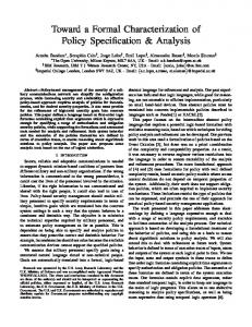
The two ensemble approaches discussed in Sections III and IV were tested via simulation. To our knowledge, there exists no publicly available, real or simulated, data set containing multi-stage cyber attacks. Simulated multi-stage attacks were generated using the simulator developed by Kuhl et.al. [21] on two networks, shown in Figures 6 and 7. The two networks were designed to represent two types of enterprise networks. Network A represents the case where each service is implemented in only one or few dedicated servers, while Network B implements about 10 instances per service. Network B also has more total machines and service types, representing a larger network with a more redundant configuration. Both networks were configured with firewall rules restricting traffic between different parts of the network. The entire sets of rules are too large to be included in this paper, but the general idea is that the departments (shaded boxes in the figures) that have their own servers or reside deeper in the network will have more restricted rules. A total of 1,000 random attacks containing 6,854 alerts were generated for Network A, and 1,500 attacks, composed of 11,697 alerts, were generated for Network B. The data set contains a mixture of ‘stealthy’ attacks where some steps are not observed, and attacks with different ‘efficiency’ level. An

of capability and opportunity assessment (TBM-CO) and the Fuzzy combination of VLMM predictions (F-VLMM). The results show that both algorithms work well for Network A, and F-VLMM outperforms TBM-CO in terms of the average performance and particularly for Network B. TABLE V P ROJECTION PERFORMANCE , [lower, upper], ACHIEVED BY TBM-CO AND F-VLMM FOR THE VARIOUS DATASETS . Net A TBM-CO F-VLMM

Fig. 6. Network A: 6 subnets, 11 servers and 4 clusters of hosts (24 hosts total), containing 31 services (15 types total), interconnected via 4 routers.

Fig. 7. Network B: 9 subnets, 23 servers and 8 clusters of hosts (130 hosts total), containing more than 300 services (37 types total), interconnected via 8 routers.

[75%,80%] [81%,88%]

High Eff. [59%,79%] [85%,88%]

Net B Medium Eff. [55%,77%] [84%,88%]

Low Eff. [54%,74%] [81%,84%]

The TBM-CO performs better for Network A than it does for Network B, because Network A is designed with more restricted firewall rules and servers that have dedicated roles. The attack paths can be differentiated based on the combinations of exposed services and firewall restrictions. On the other hand, Network B has a large number of attack paths with similar firewall configurations and many services of the same type to exploit. The abundant similar attack opportunities make it difficult for the TBM-CO to differentiate among the threatened targets, and hence the lowered performance. The F-VLMM performs well for both networks and outperforms the TBM-CO because (1) the VLMM captures the attack patterns in both targeted subnets and targeted service exposures, and (2) the fuzzy combination successfully differentiates the attacked targets from other targets. Figure 8 shows the number of targets receiving different threat scores when all the targets are considered (top) and only the attacked targets are considered. The majority of attacked targets receive high threat scores. The same fuzzy functions and rules are used for different datasets, showing its robustness.

attack is most efficient if it utilizes the minimum number of stepping stones to get to the final target in the network. A number of targets were chosen for both data sets, representing a broad range of servers and hosts in different departments within the corresponding network. B. Overall Results Given the datasets, the algorithms were tested to determine whether they can accurately project the next attacked target given the already observed events. Cyber attack projection aims at providing a ranked list of projected targets, instead of a prediction of what exactly will happen next. Therefore, the performance of the algorithm was evaluated by examining the percentile ranking of the attacked target one step prior to it being attacked. Because there could be ties in the projection scores, the results presented in this paper are shown in the form of [lower, upper], representing the interval of percentile ranking of targets received the same score as the attacked target. Table V shows the average percentile rank in the datasets by running the two algorithms: the TBM-based combination

Fig. 8. The number of targets receiving different threat scores: all targets (top) vs. only attacked targets (bottom).

While it may not be obvious from the overall results, the F-VLMM generally performs better for efficient attacks. Essentially, efficient attacks use only specific stepping stones without deviating from reaching the final goal. Therefore, patterns are easier to capture. There are instances where attacks deviate from the identified patterns, and the F-VLMM could perform not as well, at least temporarily. The TBM-CO can be useful in some of these cases to keep the critical targets ranked

high. Specific case studies are presented next to illustrate the pros and cons of the two approaches. C. Specific case studies In order to provide a deeper understanding of the algorithms on different types of attacks, this section presents a case study with three attacks that target the same mail server residing in Department F in Network B. Table VI shows the attack steps (only sip and tip are shown) of a high efficiency attack. The attack starts with compromising the external mail server (Step 1-3), then tries to access an internal server (Step 4). After that, a member of the host cluster in Department A (Step 5-7) is compromised to access Department C and E, to reach the final target. TABLE VI A HIGH EFFICIENCY ATTACK WITH PERCENTILE RANK INTERVAL ACHIEVED BY F-VLMM. Step 1 2 3 4 5 6 7 8 9 10

Source IP 9.5.231.72 237.22.202.140 178.87.46.91 192.168.1.3 192.168.1.3 192.168.1.3 192.168.1.3 192.168.2.18 192.168.4.22 192.168.6.111

Target IP 192.168.1.3 192.168.1.3 192.168.1.3 192.168.2.6 192.168.2.8 192.168.2.9 192.168.2.18 192.168.4.22 192.168.6.111 192.168.7.9

Percentile Rank N/A [96.78%,100%] [93.75%,96.88%] [96.88%,100%] [96.88%,100%] [93.75%,96.88%] [93.75%,96.88%] [96.75%,96.88%] [90.63%,93.75%] [93.75%,96.88%]

Also shown in Table VI are the percentile rank intervals of the targeted machines one step before each attack. Note that this is extracted from the overall results shown in Section V-B. It is clearly evident that F-VLMM consistently performs exceptionally for this multistage attack with the percentile ranked above 90% and many ranked above 95%. This suggests that VLMM can almost perfectly capture the pattern exhibited by attacks that go straight to the target 192.168.7.9 even if it is hidden behind 4 subnets: 192.168.1.x, 192.168.2.x, 192.168.4.x, and 192.168.6.x (i.e., 3 layers of firewalls). Table VII shows the percentile rank interval achieved by TBM-CO for the same attack shown in Table VI. This is one of the attacks in the Network B dataset that TBMCO does not perform well. There are two reasons. First, as the attack progresses, the upper remains high for the Opportunity assessment but the lower keeps dropping. This can be explained by considering a network with a total of n target machines, out of which m are already compromised by an attack at a given point, and k are targets reachable from any of the compromised machines. If all reachable targets are ranked equally, the percentile rank interval will be [(n − m − k)/(n − m) × 100%, 100%]. This gives the lower and upper bounds of the percentile rank achievable by the Opportunity assessment. As an attack progresses, more targets are compromised (larger m) and more possible targets present themselves (larger k), resulting in a smaller lower bound. Second, the percentile rank achieved by the Capability assessment drops significantly after Step 2. This is due to that many services of the same type are configured on different

TABLE VII T HE BREAK DOWN OF PERCENTILE RANK INTERVAL ACHIEVED BY TBM-CO FOR THE ATTACK SHOWN IN TABLE VI. Step 1 2 3 4 5 6 7 8 9 10

Opportunity N/A [64.52%,100%] [64.52%,100%] [60%,100%] [42.3%,100%] [42.3%,100%] [42.3%,100%] [33.51%,100%] [28.29%,100%] [24.22%,100%]

Capability N/A [100%,100%] [100%,100%] [37.26%,56.67%] [32.88%,58.47%] [32.88%,58.47%] [32.88%,58.47%] [42.52%,68.85%] [37.72%,69.15%] [32.07%,58.27%]

TBM-Fused N/A [100%,100%] [100%,100%] [55%,56.67%] [44.71%,51.57%] [44.71%,51.57%] [44.71%,51.57%] [52.28%,59.21%] [45.53%,57.74%] [38.58,48.76%]

machines in Network B. Note that this is the percentile rank of the attacked ‘targets.’ By examining the rank of the attacked ‘service types,’ the Capability assessment actually achieves consistently good performance – around [77%,83%] for all datasets. While this service projection performance translates to good target projection performance for Network A, it does not work well for Network B because many machines contain similar services. Although both the Opportunity and Capability assessments have their limitations, the TBM-based combination effectively resolves conflict and narrows the percentile interval as shown in Table VII. As the individual assessments improves, TBM will serve well as a combination technique to project cyber attacks. Table VIII shows a ‘less efficient’ attack that has the same final target 192.168.7.9 as the previous attack. The projection performance by F-VLMM is significantly lower for Steps 5, 9, 10, 13, and 14. Step 9 attempted to attack the server 192.168.2.2 while it has already penetrated deeper into 192.168.4.x subnet. Typically such an activity is done prior to further penetration attempts. For Steps 10 and 13, the attack probes into Subnets 192.168.5.x and 192.168.3.x even though they do not contain the target machine. The majority of the dataset, however, contains high efficiency attacks and the model adaptively trained will not rank those seemly unrelated victims high. Because a wide variety of subnets have been visited, F-VLMM is not able to project accurately the real target, and, hence, performs poorly in the final step. While the F-VLMM can be misled by this attack due to low efficiency (or purposely executed by the attacker to mislead the algorithm), the TBM-CO does not drop the rankings for the targets in those misleading steps - achieving between 50% and 65% percentile ranking. The advantage of TBM-CO is that it will not be affected by the pattern shown in the attack, and thus will not be misled by deviating or decoy attacks. Table IX illustrates a stealthy attack that has the same target as the previous cases, but can perform some intermediate steps without being detected. There is one or more missing steps between Steps 3 and 4. Step 3 compromised 192.168.2.7, but Step 4 shows an internal machine 192.168.2.9 being used as a stepping stone. Assuming there is no insider threat, 192.168.2.9 must be compromised before it attacks 192.168.4.20, which, in turns, is used to attack other machines.

TABLE VIII A LOW EFFICIENCY ATTACK WITH PERCENTILE RANK INTERVAL ACHIEVED BY F-VLMM. Step 1 2 3 4 5 6 7 8 9 10 11 12 13 14

Source IP 9.5.231.72 237.22.202.140 178.87.46.91 192.168.1.3 192.168.1.3 192.168.1.3 192.168.2.9 192.168.2.9 192.168.2.9 192.168.2.2 192.168.2.2 192.168.4.40 192.168.2.2 192.168.6.5

Target IP 192.168.1.3 192.168.1.3 192.168.1.3 192.168.2.6 192.168.2.6 192.168.2.9 192.168.4.35 192.168.4.16 192.168.2.2 192.168.5.5 192.168.4.40 192.168.6.5 192.168.3.17 192.168.7.9

Percentile Rank N/A [90.63%,93.75%] [93.75%,96.88%] [96.88%,100%] [50.00%,53.13%] [84.38%,87.50%] [81.25%,84.38%] [96.88%,100%] [37.5%,40.63%] [40.63%,43.75%] [84.38%,87.5%] [84.38%,87.5%] [18.75%,21.88%] [3.13%,6.25%]

Because the data is generated via a simulator that contains ground truth of the attack, we know there is no insider threat and there is indeed an attack step not being detected. TABLE IX A STEALTHY ATTACK WITH PERCENTILE RANK INTERVAL BY F-VLMM. Step 1 2 3 4 5 6

Source IP 9.5.231.72 237.22.202.140 192.168.1.3 192.168.2.9 192.168.4.20 192.168.6.113

Target IP 192.168.1.3 192.168.1.4 192.168.2.7 192.168.4.20 192.168.6.113 192.168.7.9

Percentile Rank N/A [96.88%,100%] [96.88%,100%] [75%,78.13%] [75%,78.13%] [81.25%,84.38]

The missing step has affected the F-VLMM in recognizing the pattern and thus the projection is not as accurate as in the first case. Interestingly, the projection percentile rank become better again in the final step because the pattern resurfaces from Steps 4 and 5. The TBM-CO performs comparable in this case. VI. C ONCLUSION Moving beyond intrusion detection, cyber security can benefit from projection of multistage cyber attacks, where likely future targets can be identified for timely responses. Projecting cyber attacks requires extraction and analysis of various characteristics, including capability, opportunity, and history of patterns exhibited in attacks’ progression in the network. While previous work introduced attack assessments based on these characteristics, this paper revisited them and presented two ensemble techniques to combine the attack projection estimates. Thorough analysis via simulation were presented to provide insights toward ensemble characterization of multistage attacks. The TBM-CO utilizes logical choices of Capability and Opportunity assessment and effectively resolves conflicts using the TBM-based combination. The analysis reveals that the Capability and Opportunity assessments individually are more effective when the network has restricted firewall rules and dedicated service configuration. The F-VLMM, on the other hand, is developed to effectively capture sequential patterns

of attack progression and uses Fuzzy inference to combine estimates based on subnet and services visited. Simulation results have shown F-VLMM’s superior performance, and its resilience to different types of networks and attacks. For attacks deviating from the extracted pattern due to noise, decoy, or stealthy attack actions, the F-VLMM can benefit from the TBM-CO but can also recover if the deviation is temporary. R EFERENCES [1] A. Valdes and K. Skinner, “Probabilistic alert correlation,” Recent Advances in Intrusion Detection (RAID 2001), no. 2212, 2001. [2] P. Ning, Y. Cui, and D. S. Reeves, “Constructing attack scenarios through correlation of intrusion alerts,” in Proceedings of the 9th ACM conference on Computer and communications security, 2002, pp. 245– 254. [3] F. Valeur, G. Vigna, C. Kruegel, and R. A. Kemmerer, “A comprehensive approach to intrusion detection alert correlation,” IEEE Transactions on Dependable and Secure Computing, vol. 01, no. 3, pp. 146–169, 2004. [4] S. J. Yang, A. Stotz, J. Holsopple, M. Sudit, and M. Kuhl, “High level information fusion for tracking and projection of multistage cyber attacks,” Information Fusion, vol. 10, no. 1, pp. 107 – 121, 2009. [5] J. Holsopple and S. Yang, “FuSIA: Future situation and impact awareness,” in Proceedings of 11th International Conference on Information Fusion, 2008, pp. 1–8. [6] X. Qin and W. Lee, “Attack plan recognition and prediction using causal networks,” in Proceedings of Computer Security Applications Conference, 2004, pp. 370–379. [7] D. Fava, S. Byers, and S. Yang, “Projecting cyberattacks through variable-length markov models,” IEEE Transactions on Information Forensics and Security, vol. 3, no. 3, pp. 359–369, 2008. [8] S. Vidalis and A. Jones, “Using vulnerability trees for decision making in threat assessment,” University of Glamorgan, School of Computing, Tech. Rep. CS-03-2, June 2003. [9] C. Phillips and L. P. Swiler, “A graph-based system for networkvulnerability analysis,” in Proceedings of the 1998 workshop on New security paradigms, 1998, pp. 71–79. [10] J. Dawkins and J. Hale, “A systematic approach to multi-stage network attack analysis,” in Proceedings of 2nd IEEE International Information Assurance Workshop, 2004, pp. 48–56. [11] Y. Liu and H. Man, “Network vulnerability assessment using Bayesian networks,” in Proceedings of Data Mining, Intrusion Detection, Information Assurance, and Data Networks Security, vol. 5812, 2005, pp. 61–71. [12] R. Lippmann, K. Ingols, and L. Laboratory, “An annotated review of past papers on attack graphs,” Tech. Rep., 2005. [13] A. Steinberg, “Open interaction network model for recognizing and predicting threat events,” in Proceedings of Information, Decision and Control, 2007, pp. 285–290. [14] P. Smets, “The combination of evidence in the transferable belief model,” IEEE Transactions on Pattern Analysis and Machine Intelligence, vol. 12, no. 5, pp. 447–458, 1990. [15] N. I. of Standards and C. S. D. Technology, “National vulnerabilities database (NVD).” [Online]. Available: http://nvd.nist.gov/nvd.cfm [16] Mitre, “Common Vulnerabilities and Exposures CVE dictionary.” [Online]. Available: http://cve.mitre.org/ [17] G. Shafer, Ed., A Mathematical Theory of Evidence. Princeton University Press, 1976. [18] S.-B. Cho and J. Kim, “Multiple network fusion using fuzzy logic,” IEEE Transactions on Neural Networks, vol. 6, no. 2, pp. 497–501, 1995. [19] B. N. Nelson, P. D. Gader, and J. M. Keller, “Fuzzy set information fusion in land mine detection,” in Proceedings of Detection and Remediation Technologies for Mines and Minelike Targets IV, vol. 3710, no. 1, 1999, pp. 1168–1178. [20] H. Nguyen and M. Sugeno, Fuzzy systems: modeling and control. Kluwer Academic Pub, 1998. [21] M. Kuhl, J. Kistner, K. Costantini, and M. Sudit, “Cyber attack modeling and simulation for network security analysis,” in Proceedings of Winter Simulation Conference, 2007, pp. 1180–1188.