We present a reservoir simulation scheme that gives accurate resolution of both ... we aim towards a numerical scheme that facilitates reservoir simulation of ...
1
Toward reservoir simulation on geological grid models JØRG E. AARNES and KNUT–ANDREAS LIE SINTEF ICT, Dept. of Applied Mathematics, P.O. Box 124 Blindern, NO-0314 Oslo, Norway
Abstract We present a reservoir simulation scheme that gives accurate resolution of both large-scale and fine-scale flow patterns. The method uses a mixed multiscale finite-element method (MMsFEM) to solve the pressure equation on a coarse grid and a streamline-based technique to solve the fluid transport on a fine-scale subgrid. Through this combination, we aim towards a numerical scheme that facilitates reservoir simulation of large heterogeneous geomodels without upscaling. We validate the method by applying it to a 3D upscaling benchmark case taken from the 10th SPE Comparative Solution Project. The numerical results demonstrate that the combination of multiscale methods and streamlines is a robust and viable alternative to traditional upscaling-based reservoir simulation.
1. Introduction The size of geomodels used for reservoir description typically exceeds by several orders of magnitude the capabilities of conventional reservoir simulators. These simulators therefore employ upscaling techniques that construct coarsened reservoir models with a reduced set of geophysical parameters. This way the size of the simulation model is reduced so that simulations can run within an acceptable time frame. Here we propose an alternative strategy, where the key idea is to use a mixed multiscale finite-element method (MMsFEM) [1] to discretize pressure and velocities and streamlines to discretize fluid transport. The main objective of the paper is to present a new numerical methodology that facilitates reservoir simulation of high-resolution geomodels. The model for immiscible and incompressible two-phase flow can be derived from the phase continuity equations
(1) and Darcy’s law that relates the phase velocities
to the gradient of the phase pressures
(2) Here denotes porosity; is the saturation of phase ; is a source term representing wells; is the rock permeability tensor, assumed to be symmetric and uniformly positive definite; models the reduced permeability experienced by one phase due to the presence of the other; is the phase viscosity; is the phase density; and is the gravity acceleration vector. Throughout, we assume that the phases are oil (o) and water (w) and that the two phases together fill the void space completely so that . Now define the phase mobility , the total mobility , and the fractional flow . Furthermore, denote by the capillary pressure, and assume that there exists an auxiliary function such that . We can then define the global pressure , and, by summing the continuity equations (1) and using that , we derive equations for and the total velocity , (3) 9th
European Conference on the Mathematics of Oil Recovery — Cannes, France, 30 August - 2 September 2004
2
To derive a mass transport equation for, say, the water phase, we need an expression for the water velocity. By a straightforward manipulation of using (2) we obtain
(4) Finally, neglecting effects from capillary forces and inserting (4) into (1), we obtain
(5) For brevity we hereafter drop the subscript from and let denote water saturation. In streamline simulation a sequential splitting is used to decouple and solve the coupled system (3)–(5). First, the initial saturation distribution is used to compute the mobilities in (3) and the equation is solved for global pressure and total velocity. Then, the total velocity is held constant as a parameter in (5), while the saturation is advanced in time. This completes one step of the method. Next, the new saturation values are used to update the mobilities in (3), the pressure equation is solved again, and so on. To run simulations on large geomodels we need an accurate and efficient scheme for solving the pressure equation (3). The MMsFEM introduced by Chen and Hou [5] generates solutions that are locally mass conserving on the coarse grid and reflect the fine-scale characteristics of the elliptic coefficients. Aarnes [1] extended the method further and developed a modified variant of MMsFEM that generates locally mass conservative velocity fields also on the subgrid scale. Local mass conservation is essential for a streamline method, and in the following we will therefore use Aarnes’ modified method. Related approaches include the multiscale finite-volume method by Jenny, Lee and Tchelepi [7], and the variational multiscale methods (see e.g., the overview by Arbogast [4] and references therein). The streamline method is outlined in Section 2 and the MMsFEM is described in Section 3. 2. A streamline method for two-phase flow simulation When solving the saturation equation (5) for two-phase flow with a streamline method, the first step is to use an operator splitting to separate gravity effects from the advective forces. Away from wells, the split equations corresponding to (5) are (6) (7) where . Equations (6) and (7) are then solved along one-dimensional streamlines and gravity lines induced by the velocity fields and , respectively. This operator splitting is also implemented in the commercial streamline simulators FrontSim and 3DSL. To describe the concept behind the streamline methodology, assume that is divergence free and irrotational, and consider the model equation (8) The corresponding streamlines are the flow-paths traced out by a particle being advected by the flow field so that the velocity is tangential to the streamline at every point. Since is divergence free, the streamlines do not cross, and each streamline can be viewed as an isolated flow system. To transform (8) into a family of one-dimensional equations along streamlines, we introduce the time-of-flight coordinate , which measures the time it takes
3
for a passive particle to travel along the streamlines with speed . Thus, along any streamline, the associated time-of-flight coordinate must satisfy the differential equation (9) Hence, by tracing the streamlines from cell-to-cell and computing the corresponding celltraversal times by integrating the latter equation in (9) along the streamlines, we obtain an irregular grid in the time-of-flight coordinate for each streamline. Finally, by invoking the operator identity , the multidimensional equation (8) reduces to a family of onedimensional equations along each streamline, (10) For regular quadrilateral or hexahedral grids, the flow paths can be traced on a cell-by-cell basis with an analytical method developed by Pollock [9]. Prevost, Edwards and Blunt [10] showed that Pollock’s method could be extended to give an inexact tracing algorithm on structured quadrilateral or hexahedral grids with irregular grid-block geometries. However, further research is needed to assess what kind of impact this tracing error has on the accuracy of the cell-traversal times, and hence on the streamline simulation scheme. Summing up, the streamline method for two-phase flow consists of the following steps. First, the streamlines with respect to (6) are traced on a cell-by-cell basis from injector to producer with a suitable tracing algorithm. This results in an irregular grid along each streamline where the size of each grid cell is equal to the traversal time through an underlying grid cell in physical space. Within each of the underlying grid cells, the initial saturation value is constant. By picking up these values, one obtains a piecewise initial value function for (6) on the streamline grid, and one can evolve the saturation along the streamlines with any suitable numerical scheme. The streamline saturation profile is then projected back onto the original grid by weighting the contributions from the individual streamlines according to the associated traversal time through the grid cells. Finally, after this procedure is repeated for all streamlines, the same method is used to solve (7), but now the gravity lines are initiated in the top layer of cells and terminated in the bottom layer of cells. 3. A mixed multiscale FEM Let denote the reservoir domain and let be the outward pointing unit normal on . For simplicity we assume that no-flow boundary conditions are imposed on . Then the mixed such that formulation of (3) reads: Find
(11) for all
and
. Here
is the function space
In mixed finite element methods, the approximation space for is spanned by a finite set of base functions . The base functions for the proposed MMsFEM are defined as follows: Divide into polyhedral (coarse grid) elements and let be the (non-degenerate) interface between two coarse grid blocks and . Then, for each interface , 9th
European Conference on the Mathematics of Oil Recovery — Cannes, France, 30 August - 2 September 2004
4
Figure 1: The x-component of two multiscale base functions associated with an interface outside the near-well region in a regular quadrilateral grid. The right and left plots correspond to homogeneous and random coefficients, respectively. we define a corresponding base function by constant) by the following “pressure equation”:
, where
is determined (up to a
(12) and no-flow boundary conditions on approximation space for the total Darcy velocity is
. Thus, the associated MMsFEM .
Figure 1 shows the x-component of two MMsFEM base functions that correspond to an interface outside the near well region (so that ) in a regular quadrilateral grid. Note that the base functions that correspond to homogeneous coefficients coincide with the associated base function for the Raviart-Thomas mixed FEM of lowest order. In contrast, we see that the base function that corresponds to random coefficients fluctuates rapidly to reflect the fine scale heterogeneous structures. Since it is important that all base functions are mass conserving, the subgrid problems must be solved using a mass conservative method, e.g., a suitable mixed FEM or a finite-volume method. The particular choice of method depends in part on the local grid structure. For instance, if we want to discretize the subgrid problems with a finite-volume method, a two-point flux approximation can be used if is a diagonal tensor and the grid is orthogonal, whereas a multipoint flux approximation scheme should be used on non-orthogonal grids. Also note that the base functions will generally be time dependent since they depend on . This indicates that one has to regenerate the base functions for each time step. However, it is usually sufficient to regenerate a small portion of the base functions at each time step since the total mobility only varies significantly in the vicinity of the propagating saturation front (cf. [1]); similar observations have been made for the multiscale finite-volume method developed by Jenny et al. [7]. 3.1 The approximation space for the pressure In the original version of the MMsFEM [5], Chen and Hou approximated the pressure using the piecewise constant approximation space . This was a natural choice since the approximation spaces for the Darcy velocity and pressure satisfied , a relation that guarantees stability. However, is changed when the base functions are altered to produce mass conservative velocity fields, and the relation is therefore not true. Based on this observation, Aarnes [1] argue that one also needs to modify the approximation space for the pressure. This can be illustrated by considering a simplified one-dimensional model without gravity forces.
5
Thus, let , neglect gravity, and let solve the (not discretized) mixed formulation (11). The definition of the base functions then implies that the velocity belongs to the MMsFEM approximation space . To see this, we write , where and is the subgrid variation that has zero average over all coarse grid blocks , and assume for a moment that is known a priori and move it to the right hand side. Then, since and , we find that is the unique pair in which satisfies
(13) From (13) we see that by assuming , we disregard the contribution from the integral . Numerical experience shows that neglecting this term can have strong impact on term the accuracy of . This indicates that it is necessary to modify the approximation space for pressure in the MMsFEM formulation. Moreover, (13) suggests that the approximation space should be close to the affine space . Unfortunately, it is not necessarily straightforward to define such an approximation space since is never known a priori. However, if , then vanishes everywhere except where . Thus, it is sufficient to find a function that approximates in the well blocks and vanishes elsewhere. To this end, recall that, by elliptic regularity, the "pressure solutions" are differentiable. and define in by Thus, if we write (14) and
then
This shows that
and that
. Finally, we have
Hence, since (13) admits a unique solution (up to a constant), it follows that in one spacedimension, the block-average pressures is obtained by solving (13) with replaced by . In other words, if is defined correctly, then and the projection of onto can be computed by solving (13). We should here add that the coupling between and implies that we cannot move to the right hand side. Instead, the integral provides a stronger coupling the integral term between and in the MMsFEM coefficient matrix. The splitting , where and is defined by (14), does not hold in higher dimensions, or if gravity forces are present, because we can in general not write as a linear combination of the multiscale base functions . However, the fact that the base functions and the corresponding subgrid pressure imply define an appropriate relationship between that should still give a good approximation to . We therefore propose to seek
Henceforth we will, for brevity, refer to this method simply as MMsFEM.
9th
European Conference on the Mathematics of Oil Recovery — Cannes, France, 30 August - 2 September 2004
6
3.2 Well-model In reservoir simulation, the well-rate distribution for each well is defined by specifying the bottom-hole pressure or the total well rate, through the use of a so-called well model. In a simple Peaceman-type well model the well rate in cell of a well is linearly related to the difference between the cell pressure and the bottom-hole pressure (15) Here the well transmissibility is defined by some semi-analytical relation [8]. Hence, if the bottom hole pressure is given, then is added to the appropriate diagonal entry in the linear system for the pressure equation, and enters into the corresponding right hand side component. If a well is rate-constrained, i.e., if is specified, then the associated bottom hole pressure is normally treated as an extra free variable, and the expanded linear system is closed by adding the extra equation
When solving the subgrid problems (12) we use the rate-constrained Peaceman well model. That is, we assume that the well-rate sum is equal to one. To define a well model for the MMsFEM at the coarse grid scale, we recall that approximates the subgrid pressure in a well block . This relation suggests that we can define a multiscale well-model based on the accumulated well-rates induced by and the (Peaceman type) well-model that is used to compute (16) Hence, if we assume that the well-rates are specified by the bottom-hole pressure and define , then the block transmissibility enters into the linear system as a diagonal component in the lower right hand block of the MMsFEM coefficient matrix and the transmissibility weighted sum enters into the right hand side. Finally, the contribution from , which is defined by (14), will enter into the lower left hand block of the MMsFEM coefficient matrix. Rate constrained wells are treated similarly by letting the bottom-hole pressure be an extra free parameter that is determined by adding an extra equation to the MMsFEM system. 4. Numerical results In this section we demonstrate that the MMsFEM-streamline approach is a robust and viable alternative to upscaling-based reservoir simulation schemes by testing it on reservoir models taken from the second test case in the tenth SPE comparative solution project [6]. The model was designed to benchmark different upscaling techniques and should therefore serve as a good test case for our methodology. The reservoir model consists of a Tarbert formation in the top 35 layers and an Upper Ness sequence in the bottom 50 layers. Both formations are characterized by large permeability variations, 8–12 orders of magnitude, but are qualitatively different, the Tarbert formation being smoother and hence easier to upscale. We neglect compressibility in our simulations, but all other parameters are as specified in [6]. A schematic of the well configuration is shown in Figure 2.
7
Figure 2: Schematic of the well configuration in the reservoir model in [6]. The reservoir dimensions are ft., and the model consists of grid cells. The multiscale-streamline (Ms-SL) methodology was tested on the full 3D model in [2]. The results presented therein show that Ms-SL produces solutions in close correspondence with a reference solution obtained by solving the pressure equation on a fine grid. Here we extract two smaller test cases from the full 3D model consisting of the top 5 layers in the Tarbert formation and the bottom five layers in the Upper Ness formation and show that the methodology can also handle structured non-orthogonal grids obtained by perturbing the grid corner points in the geological model. To be precise, we move each corner point to a random nearby with ft., ft., and ft. point Reference solutions are obtained by solving the pressure equation (3) at the subgrid scale with a multi-point flux-approximation (MPFA) scheme called the O-method [3]. The same method is used to construct the MMsFEM base functions. For the MMsFEM, we use two coarse grids consisting of and grid blocks and an upstream weighted finite volume method is used to evolve the streamline saturation profiles along the streamlines. Finally, we simulate 2000 days of production (0.73 PVI) and update the velocity field every 100 days. Figure 3 shows the total water-cut curves for the Tarbert and Upper Ness subsamples. For the unperturbed cases, the water-cut curves for Ms-SL almost match the reference solution. The lack of monotonicity arises since the water cut curves represent four producing wells. For the perturbed grids, the difference is larger. Some of the error can be contributed to inexact tracing of streamlines in combination with large time steps in the initial phase. However, we believe that the difference between the curves is mainly due the well model for MMsFEM. In fact, if the source term is specified so that the well rates for MMsFEM are the same as the well rates for the reference solution, then the corresponding water-cut curves are almost identical. That the dominating part of the error can be traced back to the well model is not surprising since the MMsFEM well-model is the only part of Ms-SL that involves an element of upscaling. Indeed, Ms-SL involves no tuning of parameters, except for choosing time steps and the coarse grid. 5. Conclusions We have thus presented a novel method for accurate resolution of both global and local flow patterns in large heterogeneous geomodels. The approach is based on a combination of a new multiscale discretization method for the pressure equation and a standard streamline method for the fluid transport equation. In the multiscale method, the pressure is computed on a coarsened grid using numerically constructed approximation spaces that incorporate the local heterogeneities of the elliptic operator on the underlying fine grid. The fluid transport equation is solved with a streamline method directly on the fine grid using Darcy velocities obtained by utilizing the subgrid structures in the mixed multiscale FEM base functions. The results show that the multiscale simulation method gives comparable accuracy to a reference solution that is obtained by solving the pressure equation at the fine scale, and the same streamline method for the fluid transport equation. The results therefore supports our claim that multiscale methods 9th
European Conference on the Mathematics of Oil Recovery — Cannes, France, 30 August - 2 September 2004
8
combined with streamlines can give high accuracy, and may become a robust and efficient alternative to traditional upscaling based reservoir simulation schemes.
Figure 3: Water cut curves after 2000 days of simulation. Acknowledgements The authors gratefully acknowledge financial support from the Research Council of Norway under grants no. 158908/I30 and 152732/V30.
References [1] J. E. Aarnes, On the use of a mixed multiscale finite element method for greater flexibility and increased speed or improved accuracy in reservoir simulation, Multiscale Model. Simul. 2 (2004), no. 3, 421–439. [2] J. E. Aarnes, V. Kippe, and K.-A. Lie, Mixed multiscale finite elements and streamline methods for reservoir simulation of large geomodels, Adv. Wat. Resour., submitted.. [3] I. Aavatsmark, T. Barkve, Ø. Bøe, and T. Mannseth, Discretization on unstructured grids for inhomogeneous, anisotropic media. part i: Derivation of the methods, Siam J. Sci. Comp. 19 (1998), no. 5, 1700–1716. [4] T. Arbogast, An overview of subgrid upscaling for elliptic problems in mixed form, Current trends in scientific computing (Z. Chen, R. Glowinski, and K. Li, eds.), Contemporary Mathematics, AMS, 2003, pp. 21–32. [5] Z. Chen and T.Y. Hou, A mixed multiscale finite element method for elliptic problems with oscillating coefficients, Math. Comp. 72 (2003), 541–576. [6] M. A. Christie and M. J. Blunt, Tenth SPE comparative solution project: A comparison of upscaling techniques, SPE 72469, url: www.spe.org/csp, 2001. [7] P. Jenny, S. H. Lee, and H. A. Tchelepi, Multi-scale finite-volume method for elliptic problems in subsurface flow simulation, J. Comput. Phys. 187 (2003), 47–67 [8] D.W. Peaceman, Interpretation of well-block pressures in numerical reservoir simulation with nonsquare grid blocks and anisotropic permeability, Society of Pet. Eng. Journal (1983), 531–543. [9] D.W. Pollock, Semianalytical computation of path lines for finite difference models, Ground Water 26 (1988), 743–750 [10] M. Prévost, M. G. Edwards, and M. J. Blunt, Streamline tracing on curvilinear structured and unstructured grids, SPE Reservoir Simulation Forum, SPE 66347, Houston, Texas, February 2001.