on lane/curb detection and tracking [1, 2, 3]. Many of these systems [1, 2] use a video camera and employ image processing techniques to extract lane/curb ...
Toward safe navigation in urban environments Cang Ye University of Arkansas at Little Rock, 2801 S. University Ave, Little Rock, AR, USA 72204 ABSTRACT This paper presents a complete system for autonomous navigation of a mobile robot in urban environments. An urban environment is defined as one having hard surface and comprising curbs, ramps, and obstacles. The robot is required to traverse flat ground surfaces and ramps, but avoid curbs and obstacles. The system employs a 2-D laser rangefinder for terrain mapping. In order to filter erroneous sensor data (mixed pixels and noises), an Extended Kalman Filter (EKF) is used to segment the laser range data into straight-line segments and isolated points. The isolated points are then compared with those points at their neighboring straight-line segments to detect discontinuity in received energy (called reflectivity value in this work). The points exhibiting discontinuity of reflectivity are identified as erroneous data and removed. A so-called “Polar Traversability Index” measure is proposed to evaluate terrain traversal property. A PTI dictates the level of difficulty for a robot to move along the corresponding direction. It enables the robot to traverse wheelchair ramps and avoid curbs when negotiating sidewalks in urban environment. The advantage of using PTI over the conventional traversability index is that the robot’s yaw angle is taken into account when computing the terrain traversal property at the corresponding direction. This allows the robot to snake up a steep ramp that may be too steep for the robot to climb if the conventional traversibility index were used. The efficacies of the PTI and the entire system have been verified by simulation and experiments with a real robot. Keywords: Laser rangefinder, mixed pixels, traversability analysis, obstacle negotiation, extended terrain map, polar traversability index.
1. INTRODUCTION Most of the existing research on autonomous navigation of mobile robot in urban environments has been mainly focused on lane/curb detection and tracking [1, 2, 3]. Many of these systems [1, 2] use a video camera and employ image processing techniques to extract lane/curb features. For an instance, Lai and Yung [1] proposed a multiple lanes/curbs detection method based on orientation and length features of lane marking and curb structures. Curb detection based on stereovision [4] is advantageous over the above methods as it provides 3-D information of the curb. However, systems using video camera(s) are sensitive to illumination condition. To overcome this disadvantage, Wijesoma et al. [3] used a 2-dimensional (2-D) Laser Rangefinder (LRF) for curb detection and tracking. Their method first segments the laser range data points using an Extended Kalman Filter and extracts curb segments based on curb features known ahead of time. The system then tracks the curb and allows the robot to follow the curb. This paper targets at a different way of guiding a mobile robot in an urban environment which is considered as one with hard surfaces and comprising curbs, ramps and obstacles. An indoor environment with flat ground, steps and wheelchair entries is also considered as urban terrain in this paper. The task of navigating a mobile robot in an urban environment is to steer the robot in such a way that it avoids a curb that blocks its way but traverses low-profile obstacle(s) and ramp(s) as necessary (e.g., moves up to a sidewalk via a wheelchair ramp). This ability is called Obstacle Negotiation (ON) in the literature. An essential component in an ON system is terrain mapping [5]. Stereovision [5, 6, 7] and 3-D LRFs [8, 9] have been widely used for this purpose. Stereovision is sensitive to illumination condition and has low range resolution and accuracy; while 3-D LRFs are costly and have slow frame rates that may affect the robot’s mobility. The author of this paper developed a cost-effective terrain mapping method [10] using a 2-D LRF. In [10] an elevation map and a certainty map were built simultaneously. A filtering method based on the continuity information of the elevation and certainty map is proposed to remove erroneous laser data points. The filter prefers linear motion or slow rotation of robot, and its performance may degrade when the robot turns quickly. In this paper, an Extended Kalman Filter is employed to segment the laser data points into straight-line segments and isolated points. The isolated points having discontinued reflectivity values are identified as erroneous data and removed. By using this data preprocessing, the performance of the terrain mapping system is enhanced.
Another important function an ON system is Terrain Traversability Analysis (TTA) which analyzes the traversal property of a terrain map. The TTA module usually transforms an elevation map into a traversability map which is then used to plan the robot motion. A representative TTA method is proposed by Gennery [11] which fits a least-square plane to a small terrain patch and uses the roll and pitch of each fitted plane, along with the residual of the fit to estimate the slope and roughness of the terrain patch. To cope with the inaccuracy of the stereovision data, the algorithm computes the covariance matrix of each data point and estimates the slope iteratively. It is therefore computationally complex. An alternative TTA method [6] is to use the Traversability Index (TI) to describe how easily the robot traverses a terrain cell. The TIs in [6] are represented by a number of fuzzy sets. In this paper, a new measure—Polar Traversability Index (PTI)—is proposed to evaluate terrain traversability along a specific direction. A PTI represents the level of difficulty to traverse along the corresponding direction and it allows a robot to snake up/down a steep ramp. This paper is organized as follows: In Section II the robot is introduced for urban navigation. In Section III a brief overview of the ON system is provided. Then, in Sections IV and V the terrain mapping and traversability analysis algorithms are detailed. In Section VI the PTI concept is presented. The simulation and experimental results are given in Section VII and the paper is concluded in Section VIII.
2. THE ROBOT PLATFORM FOR NAVIGATION A pioneer robot P3-DX [12] (Fig. 1) is used in this work. Since the robot moves on uneven terrain, its roll, pitch and yaw (Euler angles) must be sensed for position estimation and map-building. This is achieved by a 3-axis fiber optic gyro. Based on the Euler angular rate from the gyroscope and the data from the wheel encoder, the robot’s roll, pitch and yaw angles, and its X, Y, and Z coordinates (called robot pose collectively) are estimated. The pose information are then used to register the laser range data into a terrain map. The on-board computer uses a 2.0 GHz Pentium 4 processor. It acquires the laser range data from the LRF (Sick LMS 200) at 500k baud and the robot Euler rate data from the gyro at 38400 baud through a RS-422 card. The computer obtains the robot’s wheel encoder data at 115200 baud through a regular RS-232 port. These data are then used for terrain mapping and navigation. The robot motion commands are determined by the ON software based on the terrain map and used to control the robot. The onboard computer also transmits the robot pose and laser range data to an offboard laptop computer via the wireless router. The process of terrain mapping and navigation is thus visualized on the laptop computer in real-time.
(a) Side view of the robot
(b) Front view of the robot
(c) Laptop for remote visualization
Fig. 1. The P3-DX robot equipped with sensors for mapping and navigation
3. OVERVIEW OF THE NAVIGATION SYSTEM As depicted in Fig. 2, the navigation system consists of three main modules: Terrain Mapping, Terrain Traversability Analysis (TTA) and Path Planning. The sensor for terrain mapping is the LRF (SICK LMS 200) which is mounted on the front-end of the robot. The LRF looks forward and downward at the terrain with an angle of -10° from the robot base plate. While the robot is in motion, the fanning laser beams profile the terrain ahead of the robot and produce a terrain map. In our system, a 2.5-D grid-type terrain map is used for ON. The TTA module transforms the terrain map into a traversability map where each cell holds a value representing the degree of difficulty for the robot to move across that cell. This value is called Traversability Index (TI). The Path Planning module converts the traversability map into a number of PTIs each of which represents the level of difficulty
for the robot to move along the corresponding direction. Based on the PTIs, the Path Planning module determines the steering and velocity commands for the robot and sends these motion commands to control the robot.
Fig. 2. Diagram of the navigation system: the module within the dashed lines is the Terrain Mapping module
4. TERRAIN MAPPING AND TERRAIN MAP Terrain mapping is a process of transforming laser range measurements to 3-D points in the world coordinate (also called navigational frame) and registering these data points into a terrain map. Since laser range data may be corrupted by mixed pixels and noises, a data preprocessing process is performed in this work to enhance the quality of the terrain map. The preprocessing is based on the characteristics of the LRF.
(a) Range data
(b) Reflectivity data
Fig. 3. Range and reflectivity values of mixed pixels at various positions of the front object. The front object (black) and background object (white) were located about 2.5 meters and 3.5 meters away from the LRF. The front object was initially at the critical position outside the laser beam. It was then moved to the right step by step (1 mm each step) to produce mixed pixels.
4.1 Characteristics of the LRF and preprocessing of laser data As reported in [10], a mixed pixel may produce a range error between 20 cm and 160 cm. This error corrupts the terrain map and may deteriorate the performance of the robot in autonomous navigation. When a laser beam locates at the edge of an object, part of bean is reflected by the edge and part by the background object. The resulting range measurement lies somewhere between the edge and the background. This means that a mixed pixels exhibit a discontinuity in range measurement. In order to find out a way to remove mixed pixels, the LRF’s range and reflectivity (representing received energy) at mixed measurements are investigated. Figure 3 displays the measurements of range and reflectivity with the laser beam shooting at different positions of at the edge of the front object. It can be observe that: (1) a mixed pixel has distinctive range discontinuity; and (2) for those mixed pixels with large range discontinuity (labeled in area c), the reflectivity values are much larger than that of the front and background objects. These two features can be taken as the signature of a mixed pixel and used to remove the mixed pixel. Taking the case in Fig.3 as an example, if the threshold
value in Fig. 3b is used, then the measurements taken with the front object at position 6-11 will be identified as mixed pixels and removed, i. e., a measurement falling into area c of Fig. 3a will be removed as a mixed pixel. This treatment removes a mixed pixel with a range error bigger than 15 cm. For noises, they may also display discontinuities in both range and reflectivity due to the random nature. However, their reflectivity/range values may be smaller/bigger than that of the front and background objects. α - LRF tilt angle LRF
Ln
δ δ
p3
li+2 li+1
p2
li p1
(a) Diagram of data points on flat ground
(b) 3-D point cloud map
(c) Scene for mapping
Fig. 4. Consecutive range data points form a straight-line on flat ground. (a) three consecutive data points form a straightline on a flat ground. (b) data points collected from 311 scans represented in 3-D point cloud encoded by the reflectivity values, the brighter the point the bigger the reflectivity value. (c) the scene of the environment where data in (b) were collected.
To detect the range discontinuity, the laser range data need to be segmented. The problem of segmenting the laser range data into point sets of edge lines is formulated as an Extended Kalman Filter (EKF) similar to [16]. The EKF method⎯based on a stochastic framework⎯effectively segments and identifies isolated pixels (potential mixed pixels or random noises) simultaneously. Considering the case that three consecutive laser data points, p1, p2, and p3 forms a straight-line segment Ln on a flat ground surface, as shown in Fig. 4a, we have
li + 2 =
li li +1 . 2li cos δ − li +1
(1)
Let state variables x1(k)=li+1 and x2(k)=li, we obtain a two-sate nonlinear process model as follows:
x1 (k + 1) =
x 2 ( k ) x1 ( k ) + w1 ( k ) 2 x 2 ( k ) cos δ − x1 ( k )
(2)
x 2 ( k + 1) = x1 ( k ) + w2 ( k ) It can be written in the following vector form:
x( k + 1) = F( x( k )) + w( k )
(3)
where w(k) is the process noise and is assumed to be N ∼ (0, Q). By expending F(.) as a Taylor series about the prediction xˆ ( k | k ) at time step k and neglecting higher order terms, we linearize the process model as
Δx( k + 1) ≈ AΔx( k )
(4)
where Δx(k+1)=x(k+1)-x(k) and A is the Jabobian matrix given by
⎡ 2 xˆ 22 ( k ) cos δ A = ⎢ ( 2 xˆ 2 ( k ) cos δ − xˆ1 ( k )) 2 ⎢ 1 ⎣ The linear range measurement equation is
⎤ − xˆ12 ( k ) 2⎥ ( 2 xˆ 2 ( k ) cos δ − xˆ1 ( k )) ⎥ 0 ⎦
(5)
⎡ x (k ) ⎤ z ( k ) = li +1 = [1 0]⎢ 1 ⎥ + v ( k ) = Bx( k ) + v ( k ) ⎣ x2 ( k ) ⎦ where B is the observation matrix, and v(k) is the measurement noise which has a Gaussian distribution N ~ (0, [17] and is uncorrelated. The range data are then segmented into collinear point sets by the following EKF process:
(6)
σ r2 )
(1) The predicted measurement and the posteriori error covariance matrix are computed by
xˆ ( k + 1 | k ) = F( xˆ ( k | k )) P( k + 1 | k ) = AP( k | k ) A T + Q
(7)
(2) The innovation of the EKF is yk = Bxˆ ( k + 1 | k ) − z ( k + 1) . Assuming that the errors of the predicted
Bxˆ ( k + 1 | k ) and the observation z ( k + 1) are statistically independent, the innovation covariance T 2 is S k = B k Pk |k −1B k + σ r . The square of the Mahalanobis distances ζk between the predicted measurement and
measurement
observation is given by
ζ k = ( z (k + 1) − Bxˆ (k + 1 | k ))T Sk−1 ( z ( k + 1) − Bxˆ (k + 1 | k ))
(8)
We want to test the hypothesis H0: the predicted measurement and the observation represent the same point, i. e., yk=0. We accept the hypothesis H0 with confidence γ using a threshold value ε such that P{ζk ≤ ε | H0}= γ. In other words, the new data point z(k+1) is classified to be in the same process at a confidence of γ if ζk ≤ε. As ζk has a χ2 distribution, an appropriate threshold ε can be determined using a χ2 table. For an instance, we declare z(k+1) to be in the same process with a confidence of 0.95 if ζk ≤3.84 (ε=3.84). The filtering process continues until the event ζk >ε where the new data point is taken as an initial observation of a new process. In such an event, we take the previously filtered point as the end of the current collinear segment, and start a new process using the new measurement point as the starting point of the coming segment. (3) The Kaman Filter Gain is updated by
K ( k + 1) = P( k + 1 | k )BT Sk−1
(9)
and the state vector and the posteriori state error covariance are updated by
xˆ ( k + 1 | k + 1) = xˆ ( k + 1 | k ) + K ( k + 1) y k P( k + 1 | k + 1) = P( k + 1 | k ) − K ( k + 1)BP( k + 1 | k ).
(10)
P( k | k ) and xˆ ( k | k ) are approximately chosen using the initial two range measurements at k=1 and k=2 of each process. The filter is initialized with
⎡σ r2 0 ⎤ ⎡ z ( 2) ⎤ xˆ ( 2 | 2) = ⎢ ( 2 | 2 ) = and P . ⎢ ⎥ 2⎥ 0 σ ⎣ z (1) ⎦ r ⎦ ⎣
The range data of each laser scan are segmented into straight-line segments if there are least three collinear data points in the same process and identified as isolated points otherwise. The reflectivity value of each isolated point is then compared with that of its left and right neighboring straight-line segments. If abrupt changes (a difference bigger than 300) are detected in both sides, the point is identified as an erroneous one and thus removed. In a cluttered environment consists of many thin objects, the performance and the above method may be degraded as there are too many isolated data points. The problem will be handled by a filtering method in [10] which will be briefly described in Section 4.2. 4.2 Extended terrain map In this work, an Extended Terrain Map (ETM) is first built. Each ETM consists of an elevation map (also called a terrain map) and a so-called “certainty map.” Both are 2.5-D grid-type maps. Each cell in the elevation map holds a value
representing the height of the object at that cell; while each cell in the certainty map holds a value representing the certainty that the corresponding cell in the elevation map is occupied by the object. Homogeneous coordinate transformation is used to convert a range measurement into a point in the navigational frame. Figure 5 depicts the coordinate systems used for terrain mapping. The left figure depicts the diagram of the robot and the right figure details the coordinate systems fixed on the robot body. In Fig. 5, xbybzb is the robot body frame fixed to the midpoint of the wheel axel. Frames xsyszs and xlylzl are the coordinate systems fixed to the LRF’s mounting bracket and the LRF, respectively. The origin of frame xsyszs locates at (0, m, g+h) in frame xbybzb. The angle between zs and zl is α which is the LRF’s initial tilt-down angle, i.e., -10°. Frame xryrzr is the coordinate system attached to the laser receiver and its origin locates at (0, b, p) in frame xlylzl. The navigational frame xnynzn is aligned with the robot body frame when a navigation task is specified and it remains constant throughout the entire navigation task. The origin of the robot body frame is at (u, v, w) in the navigational frame. The three Euler angles are defined as follows: roll (φ), pitch (θ) and yaw (ψ) which are the rotation angles around yb, xb, and zb axes, respectively.
zn
rear
xn Robot
xp .
h
xs
g
zb
yp front
(u,v,w)
xb θ
zs zl
ys
Ψ m
yn
zs
zb zp
base plate
h
y φ b xb
wheel
α (0,m,g+h)
m yb xl xs
p b
xr
β
ys
zr yr
yl
d
Fig. 5. The coordinate systems for terrain mapping and navigation
The homogeneous transformation matrix Tr = [ qij ] for 1≤i≤4 and 1≤j≤4 can be derived through successive rotations n
and translations from frame xryrzr to xnynzn. The derivation is omitted here for conciseness. Apparently, Trn is a function of u, v, w, φ, θ and ψ. A range measurement l is transformed into a point (xn, yn, zn) in the navigational frame by
⎧ xn = q11l cos β + q12l sin β + q14 ⎪ ⎨ yn = q21l cos β + q22l sin β + q24 . ⎪ z = q l cos β + q l sin β + q 31 32 34 ⎩ n
(11)
For every two consecutive measurements (at time steps t and t+1) on the object at the same location (xn, yn), the expected change in height value Δz should not be bigger than t Δzmax = Δu tan φ − Δv tan(θ + α ) + Δw +
∂zn Δψ ∂ψ
∂z ∂z ∂z + n Δθ + n Δφ + n δl ∂θ ∂φ ∂l
(12)
where δl is the maximum measurement error of the LRF (32 mm according to [10]); Δu, Δv, Δw, Δφ, Δθ and Δψ are the changes in the robot’s pose from t to t+1. ∂zn⁄∂ψ, ∂zn⁄∂θ, ∂zn⁄∂φ and ∂zn⁄∂l, are the partial derivatives and they can be derived from (11). In this paper, a grid cell size of 80×80 mm is used. The height value of cell (i, j) in the elevation map is denoted by hi,j, while the certainty value of this cell in the certainty map is denoted by ci,j. Using the above transformation, a range data is translated into a point (xn, yn, zn). In order to register this point into the map at the associated location, the coordinate values xn and yn are converted to the grid indices i and j, respectively. Then the certainty value ci,j and height value hi,j of the cell in the terrain map are updated. Specifically, ci,j is updated by
t +1 i, j
c
⎧⎪cit, j + a =⎨ t ⎪⎩ci , j
t if znt +1 − hit, j ≤ Δzmax or cit, j = 0
otherwise
(13)
where a≥1 is the increment of the certainty value and it can be any positive integer. In this study the certainty value is represented by one byte and a=3 is used. As a result, all cells illuminated more than 84 times have the same certainty value. The height value hi,j of the cell in the elevation map is updated by t +1 i, j
h
⎧⎪ znt +1 =⎨ t ⎪⎩hi , j
if znt +1 > hit, j or cit, j = 0 otherwise
(14)
ci,j and hi,j are initially zero and updated by (13) and (14), respectively. In every 13.3 milliseconds the 181 range t measurements of the LRF are mapped into both maps. In (13), the condition znt +1 − hit, j ≤ Δzmax is called motion
continuity constraint [10]. Every two consecutive measurements on a real object at the same location should satisfy this constraint. According to (13), cells occupied by real object are assigned continuous certainty increments and result in large certainty values. Therefore, they can be identified easily. Mixed pixels and random noise, on the other hand, don’t satisfy the motion continuity constraint and thus result in small certainty values. In addition, they are spatially isolated in the elevation map. These characteristics can be used to filter out mixed pixels and random noises. Details of the filtering method are referred to [10]. In this work, the filtering method is applied to the laser data to remove the mixed pixels and random noise on-the-fly.
5. TERRAIN TRAVERSABILITY ANALYSIS The task of TTA is to transform a terrain map into a traversability map by assigning a TI value to each cell in the terrain map. This process is divided into two steps: estimating terrain slopes and roughness, and computing the TI value for each cell. Suppose that the Robot Geometric Center (RGC) is located at cell (i, j). A square terrain patch P centering at RGC is then formed in the terrain map. P has a side length of 2L+1 cells, where L is a positive integer. In this paper, P is chosen in such a way that it exactly envelops the robot regardless of the robot’s orientation. We then fit a least-square plane to P. The normal to the least-square plane n= (nx, ny, nz) and the residual of the fit σ can be found by the Singular Value Decomposition (SVD) method [13]. The TI value of cell (i, j) is determined based on n and σ. In the author’s recent work [14], a TTA scheme that computes a cell’s TI using the slope of the terrain patch and the residual has been implemented in a Segway robotic mobility platform. The disadvantage of the method is that it doesn’t reflect the fact that the level of difficulty for a robot to traverse a slope is related to the robot’s yaw angle. To account for this, an alternative method is proposed. As the method computes a TI along a specific direction, the robot yaw angle ψ is known. Considering that the robot is on the fitted plane, the roll and pitch of the robot can be estimated by:
⎧⎪φ = sin −1 ( n x cosψ + n y sinψ ) ⎨ −1 ⎪⎩θ = sin (( n x sinψ − n y cosψ ) cos φ )
(15)
The TI value of cell (i, j) is then calculated by
τ i , j = F1 max(| φ |, | θ |) + F2σ / N
(16)
Eq. 15 allows the robot to snake up/down a steep ramp. F1 and F2 in Eq. 16 are chosen by simulation runs in typical urban environments. In this paper, F1=3.7 and F2=0.15 are used and this set of parameters results in the roughness having a larger contribution than the slope. Apparently, the TTA process expands the obstacle’s boundaries in order to account for the dimensions of the robot. This allows us to treat the robot as a single point in planning the robot motion.
6. THE PTI HISTOGRAM FOR PATH PLANNING The path planning algorithm determines the robot’s next heading direction and velocity based on the traversal property of the local terrain map surrounding the robot. In this work, the traversal property is described by the Polar Traversability Index (PTI). In order to compute PTIs, a square-shaped local traversability map S* obtained by the above TTA method is formed at the RGC. There are ws×ws cells in S* and the RGC is at the center of S*. Figure 6 is the traversability map obtained by applying the TTA method to a computer generated elevation map. A white grid in Fig. 6 represents a cell with zero TI while the other grids represent cells with nonzero TIs. A cell with nonzero TI in the traversability map generates an imaginary vector field, which exerts a virtual repulsive force on the robot and pushes it away from the cell. This is called the “traversability field” that is defined in terms of a direction and a magnitude computed in the same way as in [15].
Fig. 6. Transformation of a traversability map into PTIs: Xn and Yn axes represent the world coordinates; o is the RGC. For simplicity, each sector is drawn in 10° and only half of the sectors are shown.
The direction of the traversability field generated by cell (i, j) is given by
ε i , j = tan −1
y j − yo xi − xo
(17)
and the magnitude of the traversability field is
mi , j = τ i2, j ( d max − d i , j )
(18)
where xi and yj are the coordinates of cell (i, j); x0 and y0 are the present coordinates of the RGC; τ i, j is the TI value of cell (i, j); dmax is the distance between the vertices (the four farthest cells) of S* and the RGC; and d i , j is the distance between cell (i, j) and the RGC. In Eq. 18, τ i, j is squared such that the impact of a cell with a small/large TI value is diminished/magnified. Obviously, mi , j decreases with increasing d i , j and it is zero for each vertices of S*. In order to evaluate the overall difficulty for the robot to traverse the terrain along a direction, the magnitude of the traversability field produced by all cells in the same direction should be summed up. For this reason, S* is divided into n sectors, each of which has an angular resolution of ξ=360°/n. Each sector k, for k = 0, L , n − 1 , has a discrete angle ρ=kξ. Cell (i, j) in S* is assigned to the kth sector according to
k = int(ε i , j ξ ) For sector k, the magnitude of the traversability field produced by all cells in this sector is calculated by
(19)
hk = ∑ mi , j
(20)
i, j
hk is the distance-weighed sum of the squared TIs of all cells in sector k. Apparently, a larger value of hk means that direction ρ=kξ is harder for the robot to move along with. In other words, hk is a TI representing the overall difficulty of traversing the terrain in the corresponding direction. Therefore, it is called the Polar Traversability Index (PTI). In this paper ξ=5°, i.e., there are 72 sectors. The PTIs are represented in a form of histogram (see Fig. 7). The path planning method then clusters the histogram into candidate valleys (which comprise consecutive sectors with PTIs below a threshold) and hills (which comprise consecutive sectors with PTIs above the threshold). A winning valley is selected among the candidate valleys to compute the robot’s next heading direction. The path planning method determines the robot’s next heading direction in such a way that it results in a trajectory with a finite length and a smooth robot motion. Eventually, the control commands⎯the velocity and steering rate commands⎯are determined and sent to the robot. The motion control uses these commands to steer the robot into the winning valley. The details of the path planning method are referred to [14].
7. SIMULATION AND EXPERIMENTAL RESULTS 7.1 Simulation results The efficacy of the PTI for urban terrain navigation is first tested in simulated urban environments. A simulator capable of generating arbitrary urban terrain was developed for the simulation study. The simulator simultaneously renders the animation of the robot traversing the terrain and the PTI histograms in real-time. Figure 7 shows one of the runs over the simulated urban terrains. The run started at S1 and terminated at target G1. Figure 7a depicts the simulated urban terrain which contains curbs (height=12 cm) and two ramps. The robot moved straightly toward the target in segments S1→1, 3→4 and 6→G1. At point 1 and 4, the curb created a peak in the PTI histogram (Figure 7b depicts the histogram at point 1) and this initiated the obstacle avoidance from 1 to 2 and from 4 to 5. At point 2 and 5, the ramp generated a winning valley in the histogram (Figure 7c depicts the winning valley V2 at point 2). The path planning algorithm started aligning the robot’s heading direction with the ramp and guided the robot passing through the ramp. Eventually, the robot came to a full stop at target G1.
(b) Histogram at point 1
(c) Histogram at point2 (a) Urban terrain and the robot trajectory Fig. 7. A run from S1 to G1 on simulated urban terrain: Kt−target direction, Kh−robot heading direction, L/R−left/right border of a candidate valley, t−time step, Vel−velocity; Yaw−robot yaw angle.
Figure 8 depicts a scenario with the robot climbing up a ramp. The ramp was too steep for the robot to move up straightly. The proposed PTI allowed the robot to snake through the ramp. At each point of S2, 2, and 4, the PTI histogram has a winning valley along the direction with a 50° yaw angle. (The target direction has a yaw angle of 90° and the robot cannot move in this direction due to the steep slope) Therefore, the robot moved up the ramp with a 50° heading direction until it reached 1 and 3 where the curb on the right generated a PTI histogram hill and blocked the robot from moving further. The robot then turned to a direction with a yaw angle of 140°. In this way, the robot snaked up the ramp to its target T2.
Fig. 8. The robot snaked up a ramp from S2 to T2
7.2 Experiments with the pioneer robot The terrain mapping system and the PTI concept have been tested with the pioneer robot on the outdoor terrain outside the Fribourgh Hall at the University of Arkansas at Little Rock. As shown in Fig. 9, the terrain is uneven and contains curbs and a ramp. A number of cardboard boxes were used to construct obstacle courses. A navigation task was specified to the robot by giving the robot its target location. The ON system was initialized by using the robot’s current position as its start point (the robot X, Y, Z coordinates are reset to zero). The ON system was implemented on the onboard computer that runs RTLinux as the Operating System. The LRF’s angular resolution was set to 1°. Each scan of the LRF takes 13.3 ms and contains 151 range data and 151 reflectivity data that cover a 150° field of view. The Real-time Data Acquisition (RDA) section in the ON system (see Fig. 2) resides in the real-time Linux kernel as a real-time thread. The RDA thread buffers the LRF data, the gyroscopic data, and the wheel encoder data in a shared memory. Once it obtains 7 scans of the laser data and the associated gyroscopic and encoder data, the Map-building and Filtering section fetches this data set, preprocess the data by the EKF method, and registered the range data into an extended terrain map. The TTA module then obtains the local terrain map (55×55 cells) and transforms it into a traversability map. Then the path planning module converts the traversability map into a PTI histogram, determines the robot’s next heading direction, computes the motion commands, and sends these commands to control the robot. The above process repeats every 93.3 ms (7×13.3 ms) until the robot reaches the target. The robot pose information (essential to terrain mapping and target seeking) were obtained by a sensor fusion method that estimates the robot roll, pitch and yaw angles, and X, Y, Z coordinates based on the encoder data and gyroscopic data (the Euler rate). The sensor fusion method is omitted here due to space limit. Figure 9 shows one of the autonomous runs from S3 to G3 on the terrain. S3 has a higher elevation than G3. The area immediately before the ramp is a valley that is lower than the neighboring area, including S3 and G3. The 3-D terrain map (rendered on the remote laptop computer) is depicted in Fig. 9b in a form of color-coded point cloud where the dark blue points represent data with negative elevation (below S3). The black spots are unperceived areas (no range data). The elevation value increases when the color changes from blue to purple and from purple to light yellow. (If displayed in a black and white picture, a brighter point has a bigger elevation value.) Figure 9c displays the elevation map at the point where the robot was avoiding the first obstacle it encountered. Figure 9e shows the elevation map at the time when the robot was avoiding the curb and aligning itself with the ramp. Figure 9f shows the elevation map after the robot successfully traversed the ramp. In the elevation maps, the unperceived areas (e.g., c) of the lower terrain surfaces look like obstacles because their Z coordinate values (zero) are bigger than that of the surrounding terrain surfaces whose elevation values are negative. Figure 9b depicts the traversability map where the obstacles (boxes) and the curbs produce impassable objects while the ramp generates a passage. The robot trajectory locates in the low-profile areas in this map. Data collected from all experimental runs has demonstrated that the roll, pitch, and yaw angles, and the velocity of the robot changed smoothly. This means that the path planning method piloted the robot on moderate terrain and produced smooth motion commands for the robot.
(a) The obstacle course on an uneven terrain
(d) 3-D terrain map: color-encoded point cloud
(b) The traversability map
(e) Avoiding the curb
(c) Avoiding the obstacles
(f) Climbing up the ramp
Fig. 9. Experiment on an outdoor terrain outside the Fribourgh Hall at UALR: The robot ran from S3 to G3. The red curve represents the robot trajectory. The robot in (b) is just for illustration. It is actually a point in the traversability map.
8. CONCLUSIONS In conclusion, this paper presents a complete system for autonomous navigation of a mobile robot in urban environments. The system employs a 2-D laser rangefinder for terrain mapping. In order to obtain high quality terrain map, laser data are filtered by two processes. In the first phase, an Extended Kalman Filter (EKF) is used to segment the data into straight-line segments and isolated points. The isolated points are then compared with those points at their neighboring straight-line segments to detect discontinuity of reflectivity values. The points exhibiting discontinuity of reflectivity are identified as erroneous data and removed. In the second phase, a filtering method⎯based on the continuity information of the elevation map and the certainty map⎯is used to further process the data and remove the erroneous data that could not be identified in the preprocessing phase. A so-called “Polar Traversability Index” measure is proposed to evaluate the terrain traversal property. A PTI represents the level of difficulty for a robot to traverse the terrain along the corresponding direction. The advantage of the proposed PTI over the conventional traversability index is that the robot’s yaw angle is taken into account when computing the terrain traversal property at the corresponding direction. This allows the robot to snake through a steep ramp which may be untraversable if the conventional TI were used. The entire navigation system can be ported to any other mobile robot for terrain mapping and navigation as it only requires wheel encoder data from the robot. The system can be applied to safe navigation of mobile robots/vehicles in urban environments for transport, surveillance, patrol, search and rescue, and military missions.
ACKNOWLEDGMENTS This work was supported in part by NASA through Arkansas Space Grant Consortium under grant number UALR16800, NASA EPSCOR Planning and Preparatory Award, and a matching fund from the Office of Research and Sponsored Programs of the University of Arkansas at Little Rock.
REFERENCES 1. A. H. S. Lai and N. H. C. Yung, “Lane detection by orientation and length discrimination,” IEEE Transactions on Systems, Man, and Cybernetics−Part B: Cybernetics, vol. 30, no. 4, 2000. 2. A. Broggi, “Parallel and local features extraction: a real-time approach to road boundary detection,” IEEE Transactions on Image Processing, vol. 4. no. 2, 1995. 3. W. S. Wijesoma, K. R. S. Kodagoda, and A. P. Balasuriya, “Road-boundary detection and tracking using ladar sensing,” IEEE Transactions on Robotics and Automation, vol. 20, no. 3, 2004. 4. R. Turchetto and R. Manduchi, “Visual curb localization for autonomous navigation,” Proc. IEEE/RSJ International Conference on Intelligent Robots and Systems, 2003, pp. 1336-1342. 5. C. F. Olson, L. H. Matthies, J. R. Wright, R. Li, and K. Di, “Visual terrain mapping for Mars exploration,” Proc. IEEE Aerospace Conference, 2004, pp. 127-134. 6. H. Seraji and A. Howard, “Behavior-based robot navigation on challenging terrain: a fuzzy logic approach,” IEEE Transactions on Robotics and Automation, vol. 18, no. 3, 2002. 7. C. P. Urmson, M. B. Dias, and R. G. Simmons, “Stereo Vision Based Navigation for Sun-synchronous Exploration,” Proc. IEEE/RSJ International Conference on Intelligent Robots and Systems, 2002, pp. 805-810. 8. I. S. Kweon and Takeo Kanade, “High-resolution terrain map from multiple sensor data,” IEEE Transactions on Pattern Analysis and Machine Intelligence, vol. 14, no. 2, pp. 278-292, 1992. 9. C. M. Shoemaker and J. A. Bornstein, “The demo III UGV program: a testbed for autonomous navigation research,” Proc. IEEE ISIS/CIRA/ISAS Joint Conference, 1998, pp. 644-651. 10. C. Ye and J. Borenstein, “A Novel filter for terrain mapping with laser rangefinders,” IEEE Transactions on Robotics, vol. 20, no. 5, pp. 913-921, 2004. 11. D. B. Gennery, “Traversability analysis and path planning for a planetary rover,” Autonomous Robots, vol. 6, no. 2, pp. 131-146, 1999. 12. Information of the pioneer robot P3-DX is available on-line at: http://www.activrobots.com/ROBOTS/p2dx.html 13. D. H. Golub and C. F. Van Loan, Matrix Computations, Prentice-Hall, 1986. 14. C. Ye, “Navigation a mobile robot by a traversability field histogram,” to appear in IEEE Transactions on Systems, Man, and Cybernetics⎯Part B: Cybernetics, vol. 37, no. 2, 2007. 15. J. Borenstein and Y. Koren, “The Vector Field Histogram−Fast Obstacle-Avoidance for Mobile Robots,” IEEE Transactions on Robotics and Automation, vol. 7, no. 3, pp. 278-288, 1991. 16. W. S. Wijesomer, K. R. S. Kodagoda, and A. P. Balasuria, “Road-boundary detection and tracking using ladar sensing,” IEEE Transactions on Robotics and Automation, vol. 20, no. 3, 2004. 17. C. Ye and J. Borenstein, “Characterization of a 2-D laser scanner for mobile robot obstacle negotiation,” Proc. IEEE International Conference on Robotics and Automation, 2002, pp. 2512-2518.